Modeling energy consumption in cellular networks

Abstract

In this paper we present a new analysis of energy consumption in cellular networks. We focus on the distribution of energy consumed by a base station for one isolated cell. We first define the energy consumption model in which the consumed energy is divided into two parts: The additive part and the broadcast part. The broadcast part is the part of energy which is oblivious of the number of mobile stations but depends on the farthest terminal, for instance, the energy effort necessary to maintain the beacon signal. The additive part is due to the communication power which depends on both the positions, mobility and activity of all the users. We evaluate by closed form expressions the mean and variance of the consumed energy. Our analytic evaluation is based on the hypothesis that mobiles are distributed according to a Poisson point process. We show that the two parts of energy are of the same order of magnitude and that substantial gain can be obtained by power control. We then consider the impact of mobility on the energy consumption. We apply our model to two case studies: The first one is to optimize the cell radius from the energetic point of view, the second one is to dimension the battery of a base station in sites that do not have access to permanent power supply.

I Introduction

According to the GSM Association, more than 80$\%$ of a typical mobile network operator’s energy requirements are associated with operating the network. The typical annual CO2 emissions per average GSM subscriber is now about 25kg CO2, which equates to the same emissions created by driving an average European car on the motorway for around one hour. However, the mobile industry continues to look for ways to reduce energy needs. Air conditioning is being replaced by fans or passive air flows whenever possible. Several programs are aiming to deploy solar, wind, or sustainable bio fuels technologies to 118,000 new and existing off-grid base stations in developing countries by 2012. Network optimization upgrades currently can reduce energy consumption by 44$\%$ and solar-powered base stations could reduce carbon emissions by 80$\%$. Optimization of the physical network through improved planning and the spectrum allocations for mobile broadband can also contribute to significant energy savings.

As a consequence of the previous statements, it appears clearly that energy consumption must be taken into consideration at the very beginning of the conception of cellular networks. For the development of cellular communications in emerging countries, it is necessary to be as energy conservative as possible by using the least possible number of base stations for a given quality of service. As the size of a cell covered by a given base station depends essentially on the emitting power of its antenna, the smaller the size of a cell, the less the consumed energy. However, when base stations cover a small region, many of them are necessary to cover a given region. There is thus a trade-off between the number and the coverage of each base stations. In order to fix the optimal radius of a cell, one must have quantitative models of the energy consumed at a base station in terms of positions, locations and traffic of the terminals. Furthermore, if we think about the deployment of base stations in low populated regions without power supply, base stations should be energetically autonomous, thus powered by a battery, be it solar or chemical. The energy consumed in such a situation is thus a key parameter in the building of a cellular network. These are the two questions we aim to answer in the following considerations.

Several measurement based analysis pointed out the different aspects in energy consumption (see [1, 2, 3, 4] and references therein). In [5], some models are proposed for the activity of a single terminal and the resulting energy consumption. In [6, 7], the choice of the cluster heads in Ad-Hoc networks integrates energy consumption consideration and take into account the geometry of the terminals by considering the proximity graph. In [8], energy saving motivates to use network coding in ad-hoc networks. As a conclusion, there are many investigations about how to save energy but no model seems to emerge in order to evaluate quantitatively the energy consumption. There is however one notable exception which is the paper [9]. In that work, a stochastic geometry based model for energy consumption in a cellular network is considered. It assumes that mobiles are connected to their closest base stations and introduces an energy consumption model based on the distance between base stations and mobiles, taking into account interference due to the presence of several base stations. We go further in this direction by considering a refined model for the energy consumption in an isolated cell, as it includes the energy devoted to broadcast messages (like the beacon signal) and takes into account both traffic activity and users mobility. Moreover, instead of relying on simulation results, we give as much as possible closed form formulas for different statistics of the energy consumption. This leads to qualitative results showing the importance of the path-loss exponent (see below for its definition).

This paper is organized as follows: In Section II, we recollect basic and advanced facts about Poisson point processes in general spaces. We then present the system model based on a Poisson point process including not only the positions but also the traffic activity and the mobility pattern of each user. In Section IV, we first evaluate the consumed energy for motionless users. We show, in Section V, that mobility does not change the mean value but decreases the variance of the consumed energy. Thus, as far as dimensioning is concerned, it is conservative to consider that users do not move. We apply these considerations in Section VI to two case studies: Finding the optimal radius of a cell under energy constraints and estimating the power of a battery to maintain a functioning network during a given time.

II A primer on Poisson point process

A Poisson process $N$ on the real line admits a usual description based on a sequence $(S_{n},\,n\geq 1)$ of independent exponentially distributed random variables. Denote by $\lambda$ the parameter of $S_{1}$. The atoms of a Poisson process are the sequence $(T_{n}=S_{1}+\ldots+S_{n},\,n\geq 1)$. Then, one can prove [12] that the number of points in a domain of Lebesgue measure $l$ is a Poisson random variable of parameter $\lambda l$. Moreover, given $N(D)=n$, i.e. given the number of points in $D$ is equal to $n$, the atoms of $N$ are independently and uniformly distributed over $D$. This explains the definition of a Poisson process in any dimension.

Definition 1.

$\pi_{\mu}$ a measure on the set configuration on $E={\mathbb{R}}^{d}$, is a Poisson point process (PPP) of intensity $\nu$ if for all sets $(C_{1},\cdots,\,C_{n})$ of mutually disjoint compact subsets of $E$:

$$\mathbf{P}(N(C_{1})=k_{1},\cdots,\,N(C_{n})=k_{n})\\ =\prod_{i=1}^{n}\left(e^{-\nu(C_{i})}\frac{(\nu(C_{i}))^{k_{i}}}{k_{i}!}\right).$$ (1)

If $\nu(\operatorname{\,d}z)=\lambda\operatorname{\,d}z$, $\pi_{\nu}$ is called the homogeneous Poisson point process with intensity parameter $\lambda$ on ${\mathbb{R}}^{d}$.

Actually, words for words, this definition does not need that $E$ is an ${\mathbb{R}}^{d}$-like space. For the mathematical details to work, it is sufficient to have $E$ a metric space with some weak topological properties. It is a useful point of view since it is often interesting to add some information to the location of users when these are represented by the realization of Poisson point process. For instance, one may want to add to the position of a customer, the fading and/or the shadowing he is experiencing, his traffic rate, etc. In the simplest case, all these characteristics should be independent from one user to the other and identically distributed. We then say that they are marks of the Poisson process. Under the above mentioned hypothesis of independence and identity in distribution, the process whose particles are couples $(x,\,v)$ is still a Poisson process on the product space ${\mathbb{R}}^{d}\times{\mathfrak{V}}$ where ${\mathfrak{V}}$ is the space in which the marks “live”. The intensity measure of this process is the product of $\lambda\operatorname{\,d}x$ times the probability distribution of the marks, denoted by $d{\mathcal{V}}(v)$. Many quantities we are longing to compute are expressible as a sum over the points of a realization of a deterministic function:

$$F=\sum_{x\in\eta}f(x,m)$$

where $\eta$ is a realization of $\pi_{\mu}$. The calculations of the different moments of such a functional turn to be known and resort to the Bell polynomials. The complete Bell polynomials $B_{n}(a_{1},...,a_{n})$ are defined as follows:

$$\exp\left\{\sum_{n=1}^{\infty}\frac{a_{n}}{n!}\theta^{n}\right\}=\sum_{n=1}^{\infty}\frac{B_{n}(a_{1},a_{2},...,a_{n})}{n!}\theta^{n}$$

for all $a_{1},...,a_{n}$ and $\theta$ such that all above terms are correctly defined. The first four Bell complete polynomials are given as:

$$B_{1}(a_{1}) = a_{1}$$

$$B_{2}(a_{1},a_{2}) = a_{1}^{2}+a_{2}$$

$$B_{3}(a_{1},a_{2},a_{3}) = a_{1}^{3}+3a_{1}a_{2}+a_{3}$$

$$B_{4}(a_{1},a_{2},a_{3},a_{4}) = a_{1}^{4}+4a_{1}^{2}a_{2}+4a_{1}a_{3}+3a_{2}^{2}+a_{4}$$

Theorem 1 (Generalized Campbell’s formula).

Let $\nu_{\lambda}(\operatorname{\,d}x,\,\operatorname{\,d}v)=\lambda\operatorname{\,d}x\otimes\operatorname{\,d}{\mathcal{V}}(v)$ and $n$ be an integer and assume that $f\in L^{p}(E,\nu_{\lambda})$ for $p\geq n$. The moments of $F$ are given by:

$${\mathbf{E}}\left[{F^{n}}\right]=B_{n}\left(\int_{E}f(z)\operatorname{\,d}\nu_{\lambda}(z),\,\cdots,\,\int_{E}f^{n}(z)\operatorname{\,d}\nu_{\lambda}(z)\right)$$

where $z=(x,\,v)$.

Poisson point processes enjoy a lot of useful properties for thinning, superposition and displacement which roughly say that whatever one of these transformations we apply to a Poisson point process, the resulting process is still a Poisson point process with a tractable intensity measure (see [10] for complete references). In the forthcoming computations, we need a more recently established property. From [13, 14], we have the following theorem.

Theorem 2.

Let $\nu_{\lambda}(\operatorname{\,d}x,\,\operatorname{\,d}v)=\lambda\operatorname{\,d}x\otimes\operatorname{\,d}{\mathcal{V}}(v)$ and $\pi_{\nu_{\lambda}}$ be a Poisson process of intensity measure $\nu_{\lambda}$. For some function $f$ sufficiently integrable, let $F(\eta)=\sum_{x\in\eta}f(x,\,v)$ and

$$\tilde{F}(\eta)=\dfrac{F(\eta)-\int f(x,\,v)\nu_{\lambda}(\operatorname{\,d}x,\operatorname{\,d}v)}{\left({\int f(x,\,v)^{2}\nu_{\lambda}(\operatorname{\,d}x,\operatorname{\,d}v)}\right)^{1/2}}\cdotp$$

For any $p\geq 1$, let

$$m(p,\,\lambda)=(\int_{C}f^{2}(x,\,v)\nu_{\lambda}(dx,\operatorname{\,d}v))^{-p/2}\\ \times(\int_{C}|f(x,\,v)|^{p}\nu_{\lambda}(\operatorname{\,d}x,\operatorname{\,d}v).$$

Let $\mu$ be the standard Gaussian measure on ${\mathbb{R}}$ and $\mu_{3}$, the measure given by

$$d\mu_{3}(x)=(1+\frac{1}{6}m(3,\,\lambda)H_{3}(x))\operatorname{\,d}\mu(x),$$

where $H_{3}(x)=8x^{3}-12x$ is the third Hermite polynomial. Then,

$$\sup_{\|\psi\|_{\mathcal{C}^{3}_{b}}\leq 1}\left|{\mathbf{E}}\left[{\psi(\tilde{F})}\right]-\int_{\mathbb{R}}\psi\operatorname{\,d}\mu_{3}\right|\leq E_{\lambda}$$

where

$$E_{\lambda}=\left(\frac{m(3,\,1)^{2}}{6}+\frac{m(4,\,1)}{9}\sqrt{\frac{2}{\pi}}\right)\lambda^{-1}.$$

This means that for $E_{\lambda}$ small, the distribution of $\tilde{F}$ is in some sense very close to $\mu_{3}$.

III System model

For the application we have in mind, i.e. deployment of a cellular network in low populated region, one can consider an isolated cell, neglecting the interference from adjacent base stations. To simplify the computations, we consider that the region covered by the base station, hereafter called the cell and denoted by $C$, is circular of radius $R$, centered at the base station $o$. The forthcoming analysis can be extended to any bounded domain of coverage but the integrals would have to be numerically evaluated. The terminals are identified to a cloud of points, which we denote by $\eta$, whose elements are the positions of each terminal in a domain larger than $C$.

The power consumed by the battery of the base station $o$ can be divided into two parts:

• The power dedicated to transmit, receive, decode and encode the signal of any active user. The cumulative power over the whole configuration is then the sum over all terminals of the energy consumed for each one.

• The power dedicated to broadcast messages. In order to guarantee that all active users receive these messages, the power must be such that the farthest user in the cell is within the reception range (if the system performs power control) or all the cell is within reception range (if the system does not perform power control). Thus, the power is a function of the maximum distance between the base station and the terminals or it is constant if power control is not performed.

For a very simple propagation model (without fading and shadowing), the Shannon’s formula states that for a receiver located at $x$, the transmission rate is given by

$$W\log_{2}(1+P_{e}l(x)),$$

where $W$ is the bandwidth, $P_{e}$ is the transmitted power and $l(x)$ is the path-loss function. This implies that in order to guarantee a minimum rate at position $x$, $P_{e}$ must be proportional to $1/l(x)$. Usual choices of path-loss functions are of the form $l(x)=\left|x\right|^{-\gamma}$ (singular path-loss model) or $l(x)=(r_{0}\vee\left|x\right|)^{-\gamma}$ or $l(x)=(1+\left|x\right|^{-\gamma})^{-1}$. The forthcoming analysis does not depend on a particular choice, so we keep it generic. It follows that for a user configuration $\eta$, the total consumed power, in presence of power control, is given by:

$$P(\eta)=\beta_{A}\sum_{x\in\eta\cap C,x\ \text{active}}l^{-1}(x)+\beta_{B}\max_{x\in\eta\cap C}l^{-1}(x)\\ :=P_{A}(\eta)+P_{B}(\eta),$$

where $\beta_{A}$ and $\beta_{B}$ are multiplicative factors defined below. The subscript A stands for "additive" and B stands for "broadcast". The term $\sum_{x\in\eta}l^{-1}(x)$ means that we add over all points $x$ of the configuration $\eta$, the value of $l^{-1}(x)$. Now, if the terminals are moving, we denote by $\eta_{t}$ the configuration at time $t$ which represents the locations of all terminals at this instant. Since the energy is the integral of the power over time, the total consumed energy between time $0$ and time $T$ is given by

$$J_{T}:=J_{T}(\eta,T)=\int_{0}^{T}P_{A}(\eta_{s})\operatorname{\,d}s+\int_{0}^{T}P_{B}(\eta_{s})\operatorname{\,d}s\\ =J_{A}(\eta,T)+J_{B}(\eta,T).$$

We should also add a constant part for the energy associated to operate the network but it doesn’t alter the statistical aspects we aim to analyze.

Figure 1: Illustration of the model, each user is associated with a ON-OFF process and a mobility process.

For years, models for the locations of users in cellular networks were left aside considering a sort of diffuse ether from which a density of calls per unit of surface and unit of time would emerge. After [10, 11], we know how to represent users locations by a Poisson point process. Note that according to the Mecke formula (2), the earlier fluid model can be viewed as a space average of this refined description. As is, one cannot expect to compute variances and higher order statistics from this model. We hereby consider that terminals are initially located according to a Poisson point process in the plane, of intensity $\lambda$: for two disjoint bounded subsets of the plane, the random variables counting the number of users in each subset are independent and Poisson distributed with parameter $\lambda$ times the surface of the subset. We enrich the Poisson point process description by adding traffic and mobility characteristics. The traffic of the user initially located at $x$, is an ON/OFF process, denoted by $A_{x}$, independent of the position of the user. We assume, as usual, that all the traffic processes of all users are independent and identically distributed. Moreover, at the beginning of the time observation window, they have all reached they stationary state (supposed to exist). We denote by $\pi_{\text{ON}}$ the probability for a given traffic process to be in its ON phase at any given time. One simple example of such a process is the exponential ON/OFF model, in which exponentially distributed ON periods alternate with exponentially distributed OFF periods. If we denote by $\mu_{\text{ON}}$ and $\mu_{\text{OFF}}$ the parameters of the exponential distributions, then $\pi_{\text{ON}}=\mu_{\text{OFF}}/(\mu_{\text{ON}}+\mu_{\text{OFF}})$. The choice of a traffic model boils down to choose a probability measure on the space ${\mathfrak{T}}$ of piece-wise, two valued, functions. We denote by ${\mathcal{T}}$ this probability measure, hence ${\mathcal{T}}(\operatorname{\,d}a)$ is the probability to have a traffic process close to the process $a$ and

$$\int H(a)\,{\mathcal{T}}(\operatorname{\,d}a)={\mathbf{E}}\left[{H(A)}\right],$$

means that we compute the mean value of a function $H$ with respect to all possible values of the generic traffic process $A$. We also envision the impact of mobility on energy consumption. We just assume that users move independently and are statistically indistinguishable: If $M_{x}$ denote the movement of user initially located at $x$, so that its position at time $t$ is $x+M_{x}(t)$, then we assume that the collection of processes $(M_{x},\,x\in\eta_{0})$ are independent and identically distributed. Besides the motionless situation where $M_{x}(t)=o$ for any $t$ and any $x$, the simplest model is that constant speed movement: $M_{x}(t)=v_{x}t$ where the vectors $(v_{x},\,x\in\eta_{0})$ are independent and identically distributed over ${\mathbb{R}}^{2}$. Choosing a mobility model boils down to determine a probability measure ${\mathcal{M}}$ on the space $\mathfrak{C}$ of continuous functions on ${\mathbb{R}}^{2}$, starting at $o$. Putting the pieces together means that we consider a Poisson process of the product space ${\mathbb{R}}^{2}\times{\mathfrak{T}}\times{\mathfrak{C}}$ with intensity $\lambda\operatorname{\,d}x\otimes{\mathcal{T}}(\operatorname{\,d}a)\otimes{\mathcal{M}}(\operatorname{\,d}m)$. In plain words, this means that a user, say located at $x$, is equipped with a traffic process $A_{x}$ and a mobility process $M_{x}$ such that all these processes are independent and identically distributed among all users.

Moreover, the so-called Mecke formula stands that

$${\mathbf{E}}\left[{\sum_{x\in\eta}\zeta(x,\,A_{x},\,M_{x})}\right]\\ =\iint\zeta(x,\,a,\,m)\lambda\operatorname{\,d}x\,{\mathcal{T}}(\operatorname{\,d}a)\,{\mathcal{M}}(\operatorname{\,d}m),$$ (2)

for any bounded function $\zeta$. The configuration of users at time $t$ is

$$\eta_{t}=\sum_{x\in\eta_{0}}\delta_{x+M_{x}(t)},$$

while the configuration of active users is

$$\sum_{x\in\eta_{0}}A_{x}(t)\,\delta_{x+M_{x}(t)}.$$

In particular, the additive part of consumed energy can be rewritten as:

$$J_{A}(\eta,T)=\sum_{x\in\eta_{0}}\int_{0}^{T}A_{x}(t)l^{-1}(x+M_{x}(t))1_{x+M_{x}(t)\in C}\operatorname{\,d}t$$ (3)

and the broadcast part is:

$$J_{B}(\eta,T)=\int_{0}^{T}\max_{x\in\eta_{t}\cap C}l^{-1}(x+M_{x}(t))\operatorname{\,d}t.$$ (4)

IV Motionless users

When users do not move, from (3), we get

$$J_{A}(\eta,T)=\beta_{A}\sum_{x\in\eta_{0}}1_{x\in C}\left(\int_{0}^{T}A_{x}(t)\operatorname{\,d}t\right)\ l^{-1}(x),$$

so that $J_{A}(\eta,T)$ appears as a shot noise process. In view of Theorem 1, we can compute easily the moments of any order of the additive part.

Theorem 3.

For motionless users, the moments of $J_{A}(\eta,T)$ are given by:

$${\mathbf{E}}\left[{J_{A}(\eta,T)^{n}}\right]=B_{n}(\alpha_{1},\cdots,\alpha_{n})$$

where

$$\mathbf{m}_{k}\left(A,T\right)={\mathbf{E}}_{{\mathcal{T}}}\left[{\left(\int_{0}^{T}A(s)\operatorname{\,d}s\right)^{k}}\right]\text{ for }k\geq 2.$$

and

$$\alpha_{k}=\lambda\beta_{A}^{k}\mathbf{m}_{k}\left(A,T\right)\int_{C}|l^{-1}(x)|^{k}\operatorname{\,d}x.$$

In particular, for the singular path-loss model,

$${\mathbf{E}}\left[J_{A}(\eta,\,T)\right]=\frac{2\beta_{A}}{\gamma+2}\,\rho\,R^{\gamma}\ T$$ (5)

where ${\mathfrak{n}}=\lambda\pi R^{2}$ is the mean number of terminals into the cell and $\rho={\mathfrak{n}}\,\pi_{\text{ON}}$ is the mean number of active customers in the cell $C$ of radius $R$.

We now show how to determine $\beta_{A}$. If $P_{e}$ denotes the power emitted by a mobile located at $x$ from the base station, since we do not take into account interference, shadowing and fading, the received power at the base station is $P_{r}=P_{e}\,K\,l(x)$ where $K=(c/4\pi fd_{ref})^{2}d_{ref}^{\gamma}$, $f$ is the frequency of the radio transmission, $c$ is the light celerity and $d_{ref}$ is the so-called reference distance. Since the base station can detect a signal of power greater than $P_{\min}^{\text{r}}$, this requires that $P_{e}$ is greater than $P_{\min}^{\text{r}}/Kl^{-1}(x)$. One can consider that the same considerations hold for the downlink channel so that $\beta_{A}=2P_{\min}^{\text{r}}/K$. In practical situation, $P_{\min}^{\text{r}}$ is of the order of $10^{-9}$ mW and $f$ around $2$ GHz, hence $\beta_{A}$ varies between $2.10^{-10}$ for $\gamma=5$ to $2.10^{-8}$ for $\gamma=3$.

On the other hand, without power control, let $P^{\prime}_{r}$ the power sufficient to ensure a reception at any point of the cell. If we denote by $P_{\min}^{\text{b}}$ the minimum power for the beacon to be detected by a mobile at distance $R$ from the base station, we should have

$$\frac{KP^{\prime}_{r}}{R^{\gamma}}\geq P_{\min}^{\text{b}}.$$

This amounts to say that we can take $\beta_{B}=P_{\min}^{\text{b}}/K$. Usually, $P_{\min}^{\text{b}}$ is around $10^{-8}$ mW. In the usual frequency bands, we obtain $\beta_{B}$ varying from $10^{-9}$ for $\gamma=5$ to $10^{-7}$ for $\gamma=3$. If there is no power control, the energy consumed for the beacon is thus equal to

$$J_{B}^{0}(\eta,\,T)=\beta_{B}R^{\gamma}T.$$ (6)

If power control is used, the power should be adjusted for the farthest terminal to be able to receive the beacon signal:

$$\frac{P_{\min}^{\text{b}}}{K}\max_{x\in\eta\cap C}l^{-1}(x)=\beta_{B}\max_{x\in\eta\cap C}l^{-1}(x).$$

Hence, in absence of movement,

$$J_{B}(\eta,T)=\beta_{B}T\ \max_{x\in\eta\cap C}l^{-1}(x).$$

Since all the usual path-loss functions depend only on the distance between $x$ and $o$, let $L$ be defined as $L(\|x\|)=l(x)$. From the remark that

$$(\max_{x\in\eta\cap C}\|x\|\leq u)=(\eta(B(o,R)\backslash B(o,\,u))=0),$$

it follows from (1) that the random variable $\delta=\max_{x\in\eta\cap C}\|x\|$ has probability density function:

$$f_{\delta}(u)=2\lambda\pi e^{-\lambda\pi R^{2}}\,u\,e^{\lambda\pi u^{2}}.$$

The next result follows.

Theorem 4.

For motionless users, with power control, the consumed energy to maintain the beacon signal, denoted by $J_{B}^{p}$ has moments given by:

$${\mathbf{E}}\left[{(J_{B}^{p}(\eta,T))^{k}}\right]=\left(\beta_{B}T\right)^{k}\ \int_{0}^{R}(L^{-1}(u))^{k}\,f_{\delta}(u)\operatorname{\,d}u,\\ \text{ for any }k\geq 1.$$ (7)

For the singular path-loss function, we obtain

$${\mathbf{E}}\left[{J_{B}(\eta,T)}\right]=e^{-{\mathfrak{n}}}{\mathfrak{n}}^{-\gamma/2}\int_{0}^{{\mathfrak{n}}}v^{\gamma/2}e^{v}\operatorname{\,d}v\ J_{B}^{0}(\eta,\,T).$$

Thus the gain of power control does depend only on the mean number of terminals whatever the radius, be it a few meters or some kilometers. Figure 2 shows that, as expected, the gain is higher for lower load.

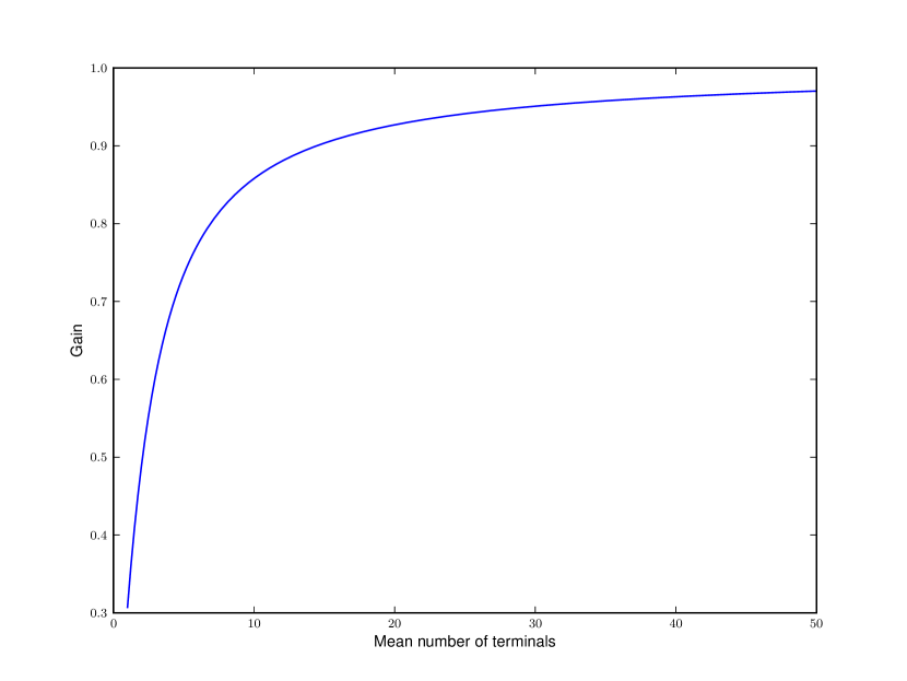
Figure 2: The energy gain with power control.

In view of (5) and (6), we have

$$\kappa:=\frac{{\mathbf{E}}\left[{J_{A}(\eta,\,T)}\right]}{J_{B}^{0}(\eta,\,T)}=\frac{2}{\gamma+2}\,\frac{\rho\beta_{A}}{\beta_{B}}=\frac{2}{\gamma+2}\frac{\rho P_{\min}^{\text{r}}}{P_{\min}^{\text{b}}}\cdotp$$ (8)

Since $\rho$, the mean number of active users is of the order of $10$ to $50$, in view of the values of $\beta_{A}$ and $\beta_{B}$, (8) says that $\kappa$ depends essentially of the ratio between $P_{\min}^{\text{r}}$ and $P_{\min}^{\text{b}}$. For the values we considered, this means that $J_{A}$ and $J_{B}$ are of the same order of magnitude.

V Impact of mobility

For the sake of simplicity for the proofs, we now assume that $J_{B}$ is constant, equal to $J_{B}^{0}$ given by (6). We now evaluate the impact of mobility on energy consumption.

According to the displacement theorem for Poisson processes, we known that for each time $t$, the point process $\eta^{\mathcal{M}}_{t}=(x+M_{x}(t),\,x\in\eta_{0})$ is a still a Poisson point process with intensity $\lambda\operatorname{\,d}x$. It follows that the expectation of consumed energy does not depend on the mobility model and is equal to the value for motionless users.

However, for higher order moments, the correlations between positions at different instants are to be taken into account so that the variance and other moments are different for truly mobile users. Let

$$\digamma_{n}^{M}(f,T)=\\ \int_{{\mathbb{R}}^{2}}{\mathbf{E}}_{{\mathcal{T}},\,{\mathcal{M}}}\left[{\left(\int_{0}^{T}f(x+M(t))A(t)1_{x+M(t)\in C}\operatorname{\,d}t\right)^{n}}\right]\operatorname{\,d}x.$$

The following theorem uses the same techniques of proof as before but in a more involved fashion.

Theorem 5.

The moments of $J_{A}(\eta,T)$ with mobility are given by

$${\mathbf{E}}_{{\mathcal{T}}}\left[{J_{A}(\eta^{\mathcal{M}},T)^{n}}\right]=\\ B_{n}(\lambda\digamma_{1}^{M}(\beta_{A}\,l^{-1},T),\lambda\digamma_{2}^{M}(\beta_{A}\,l^{-1},T),\cdots,\lambda\digamma_{n}^{M}(\beta_{A}\,l^{-1},T)).$$

It follows that mobility reduces moments of $J_{A}$; i.e

$${\mathbf{E}}_{{\mathcal{T}},\,{\mathcal{M}}}\left[{J_{A}(\eta,T)^{n}}\right]\leq{\mathbf{E}}_{{\mathcal{T}},\,0}\left[{J_{A}(\eta,T)^{n}}\right].$$ (9)

Proof:

The first part of the proof follows from Theorem 1. Let $f(x)=\beta_{A}\,l(x)\,1_{x\in C}$. Since the Lebesgue measure is translation invariant,

$$\int_{{\mathbb{R}}^{2}}f(x+y)\operatorname{\,d}x=\int_{{\mathbb{R}}^{2}}f(x)\operatorname{\,d}x.$$

If we combine that remark with Hölder inequality, we get that for $y_{1},\cdots,y_{n}$ in ${\mathbb{R}}^{2}$,

$$\int_{{\mathbb{R}}^{2}}\prod_{j=1}^{n}f(x+y_{j})\operatorname{\,d}x \leq\prod_{j=1}^{n}(\int_{{\mathbb{R}}^{2}}f(x+y_{j})^{n}\operatorname{\,d}x)^{1/n}$$

$$=\int_{{\mathbb{R}}^{2}}f(x)^{n}\operatorname{\,d}x.$$ (10)

For the sake of presentation, we denote by $\operatorname{\,d}t$ the product measure $\otimes_{j=1}^{n}\operatorname{\,d}t_{j}$ According to (V), we get

$$\digamma_{n}^{M}(f,T)\\ \begin{aligned} &=\int_{{\mathbb{R}}^{2}}\int_{[0,\,T]^{n}}{\mathbf{E}}_{{\mathcal{T}},{\mathcal{M}}}\left[{\prod_{i=1}^{n}\left(f(x+M(t_{i}))A(t_{i})\right)}\right]\operatorname{\,d}t\operatorname{\,d}x\\ &=\int_{{\mathbb{R}}^{2}}\int_{[0,\,T]^{n}}{\mathbf{E}}_{{\mathcal{M}}}\left[{\prod_{i=1}^{n}f(x+M(t_{i}))}\right]{\mathbf{E}}_{{\mathcal{T}}}\left[{\prod_{i=1}^{n}A(t_{i})}\right]\operatorname{\,d}t\operatorname{\,d}x\\ &=\int_{[0,\,T]^{n}}{\mathbf{E}}_{{\mathcal{T}}}\left[{\prod_{i=1}^{n}A(t_{i})}\right]\int_{{\mathbb{R}}^{2}}{\mathbf{E}}_{{\mathcal{M}}}\left[{\prod_{i=1}^{n}f(x+M(t_{i}))}\right]\operatorname{\,d}x\operatorname{\,d}t\\ &\leq\int_{[0,\,T]^{n}}{\mathbf{E}}\left[\prod_{i=1}^{n}A(t_{i})\right]\int_{{\mathbb{R}}^{d}}f(x)^{n}\operatorname{\,d}x\operatorname{\,d}t\\ &={\mathbf{E}}\left[\left(\int_{0}^{T}A(t)\operatorname{\,d}t\right)^{n}\right]\,\int_{{\mathbb{R}}^{2}}f(x)^{n}\operatorname{\,d}x\\ &=\mathbf{m}_{n}\left(A,T\right)\int_{{\mathbb{R}}^{2}}f(x)^{n}\operatorname{\,d}x.\end{aligned}$$

Since the coefficients of Bell polynomials are non-negative, (9) follows. ∎

We now study the limiting variance when the speed of particles is large (for instance, terminals in a high speed train). We say that a movement distribution ${\mathcal{M}}$ has property T whenever $\mathbf{P}(M(s)=M(t))=0$ for all $s\neq t$. We denote by $M^{\epsilon}$ the accelerated version of $M$ (and ${\mathcal{M}}^{\epsilon}$ the corresponding probability distribution on ${\mathfrak{C}}$): $M^{\epsilon}(t)=M(t)/\epsilon$. The full proof of the next result is given in [15].

Theorem 6.

If $M$ has the property T then in high mobility regime, the variance of $J_{A}$ tends to $0$, i.e

$${\mathbf{V}}\left[J_{A}(\eta^{{\mathcal{M}}^{\epsilon}},T)\right]\rightarrow 0\ \text{as}\ \epsilon\rightarrow 0.$$

The above results say that, when users move the total consumed energy by a base station does not change in average, and the moments of the additive part are reduced. Moreover, when users move very fast, the consumed energy during a time period is almost constant. We can see this as a consequence of weak central limit theorem. When users move faster, the configuration of users is more mixing during a same period of time, thus converge faster to the mean.

VI Applications

VI-A Dimensioning optimal cell size

Consider an operator aiming to design the optimal cell radius $R$ to cover a region of total area $S\subset{\mathbb{R}}^{2}$. We assume that the cells are circular. The average total cost of the network is assumed to be the sum of the operating cost during the life time of the network (say $T$) and the cost of facilities (base stations). We assume a fixed deployment cost for any base station regardless of its transmission range. The number of base stations is then roughly equal to $S\,R^{-2}$ so the installation cost of base stations is ${c_{1}\,S}{R^{-2}}$ with $c_{1}>0$. The operating cost is assumed to be proportional to the consumed energy.

We assume that $l$ is the singular path-loss function, i.e. $l(x)=\|{x}\|^{-\gamma}$. From the previous results, the mean energy consumed by the network during its operating time is:

$$\frac{S}{R^{2}}(1+\kappa)\beta_{B}R^{\gamma}T.$$

This is an increasing function of $R$, which means that small cell systems will consume less energy than larger cell systems. The average total cost for the network is then

$$\text{Cost}(R)=S(1+\kappa)\beta_{B}TR^{\gamma-2}+\frac{c_{1}\,S}{R^{2}}.$$ (11)

Note that $\kappa$ implicitly depends on $R$, as the larger the cell, the higher the mean number of active customers. Equation (11) shows that there are two antagonist trends: large radius cells minimize the deployment cost whereas they increase the operating cost.

If we keep $\kappa$ constant, i.e. we may have larger cell providing that the mean number of customers per unit of surface is decreasing in such a way $\lambda R^{2}$ is constant; the optimization problem has a solution obtained by differentiation:

$$R_{\text{opt}}=\left(\frac{2c_{1}}{(\gamma+2)(1+\kappa)\beta_{B}T}\right)^{1/\gamma}\cdotp$$

As expected, the optimal radius depends heavily on the value of $\gamma$ which is linked to the density of obstacles in the path of radio waves.

VI-B Dimensioning cell battery

The proposed model can be used to dimension sites that do not have access to power supply facilities. In this situation, operators have to replace or reload base station’s battery at each period $T$. We want to determine the energy level $\alpha$ of battery so that the probability of running out of energy before replacement (or reloading) be smaller than some given threshold $\epsilon$. We use results derived in the previous sections to find $\alpha$. The problem is to find $\alpha$ such that:

$$\mathbf{P}\left(J_{T}(\eta^{M},T)>\alpha\right)<\epsilon.$$

In order to simplify the problem, we assume $J_{B}$ to be constant equal to $K_{B}=\beta_{B}R^{\gamma}T$ and that the users are motionless. In view of Theorem 4, it may be thought as a pessimistic point of view without the economy due to power control. Hence, $J_{T}(\eta^{M},T)=J_{A}(\eta^{M},T)+K_{B}$. One could resort to the Bienaymé-Tcebycev inequality and use Theorem 3 to bound the variance of $J_{T}$ but this approach is known to give imprecise results. Otherwise, one can use the Gaussian approximation of Theorem 2. We can apply this theorem to the function

$$f(x,a)=\beta_{A}\ l^{-1}(x)\int_{0}^{T}a(t)\operatorname{\,d}t,$$

and hence,

$$\int_{C}\int_{{\mathcal{T}}}f(x,a)^{k}\nu_{\lambda}(\operatorname{\,d}x,\operatorname{\,d}a)=\mathbf{m}_{k}\left(A,T\right)\frac{(\beta_{A}R^{\gamma})^{k}}{\gamma k/2+1}\,{\mathfrak{n}}.$$

It follows that for any $k\geq 3$,

$$m(k,\,\lambda)=\frac{\gamma+1}{\gamma k/2+1}\frac{\mathbf{m}_{k}\left(A,T\right)}{\mathbf{m}_{2}\left(A,T\right)^{k/2}}\,{\mathfrak{n}}^{1-k/2}.$$

Since the process $A$ is supposed to be ergodic, it is well known that $\mathbf{m}_{k}\left(A,T\right)\sim(\pi_{\text{ON}}\,T)^{k}$ as $T$ goes to infinity or at least if $T$ is large compared to the cycle duration of $A$, i.e. the time between two successive communications plus the length of a communication. Since that is usually so, we get:

$$m(k,\,\lambda)=\frac{\gamma+1}{\gamma k/2+1}\,{\mathfrak{n}}^{1-k/2}.$$

Note that $m(k,\,\lambda)$ depends weakly on the geometric properties of the domain which are summarized by $\gamma$ and on the traffic pattern but mainly on the mean number of customers in the cell. The procedure is then the following: We first verify that $E_{\lambda}$ is negligible compared to $\epsilon$. Then, we solve the equation in $\alpha$,

$$\mu_{3}([\alpha,\,+\infty))=\epsilon$$

and take

$$\zeta =\mathbf{m}_{1}\left(A,T\right)\frac{\beta_{A}R^{\gamma}}{\gamma/2+1}\,{\mathfrak{n}}+\alpha\sqrt{\mathbf{m}_{2}\left(A,T\right)}\frac{\beta_{A}R^{\gamma}}{\sqrt{\gamma+1}}\,\sqrt{{\mathfrak{n}}}$$

$$\sim\left(\frac{1}{\gamma/2+1}+\frac{\alpha}{\sqrt{\gamma+1}\sqrt{{\mathfrak{n}}}}\right)\,\beta_{A}\rho R^{\gamma}T.$$ (12)

With this procedure, we get a simple way to determine the threshold $\zeta$ which guarantees that the real value of $\mathbf{P}\left(J_{T}(\eta^{M},T)>\alpha\right)$ is smaller than $\epsilon$. In Figure 3, we analyze the variations of $\zeta$ with respect to $\gamma$. Once again, we see that the provisioning of resources, i.e. energy for the time being, is exponentially dependent of $\gamma$, the path-loss exponent.

VII Conclusion

We have shown how to model energy consumption in a cellular network taking into account both communication and signaling traffic. The closed form formulas we obtained may be used for several purposes mainly in order to dimension cells or batteries under energy constraints. We pointed out the great importance of the domain geometry which is summarized by the path-loss parameter $\gamma$.

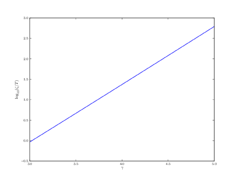
Figure 3: Variations of $\log_{10}(\zeta/T)$ with respect to $\gamma$.

References

• [1] A. Fehske, G. Fettweis, J. Malmodin, and G. Biczok, “The global footprint of mobile communications: The ecological and economic perspective,” IEEE Communications Magazine, vol. 49, no. 8, pp. 55–62, Aug. 2011.
• [2] G. Fettweis and E. Zimmermann, “ICT energy consumption - trends and challenges,” pp. 2006–2009, 2008.
• [3] X. Wang, A. V. Vasilakos, M. Chen, Y. Liu, and T. T. Kwon, “A survey of green mobile networks: Opportunities and challenges,” Mobile Networks and Applications, 2011.
• [4] M. Etoh, T. Ohya, and Y. Nakayama, “Energy consumption issues on mobile network systems,” in Applications and the Internet, 2008. SAINT 2008. International Symposium on, 28 2008-aug. 1 2008, pp. 365 –368.
• [5] K. Ullah and J. Nurminen, “Applicability of different models of burstiness to energy consumption estimation,” in 2012 8th International Symposium on Communication Systems, Networks Digital Signal Processing (CSNDSP), Jul. 2012, pp. 1 –6.
• [6] S. Chinara and S. Rath, “Mobility based clustering algorithm and the energy consumption model of dynamic nodes in mobile ad hoc network,” in International Conference on Information Technology, 2008. ICIT ’08, Dec. 2008, pp. 171 –176.
• [7] W. Heinzelman, A. Chandrakasan, and H. Balakrishnan, “Energy-efficient communication protocol for wireless microsensor networks,” in Proceedings of the 33rd Annual Hawaii International Conference on System Sciences, 2000, Jan. 2000, p. 10 pp. vol.2.
• [8] Y. Wu, P. Chou, and S.-Y. Kung, “Minimum-energy multicast in mobile ad hoc networks using network coding,” IEEE Transactions on Communications, vol. 53, no. 11, pp. 1906 – 1918, Nov. 2005.
• [9] L. Xiang, X. Ge, C. Wang, F. Li, and F. Reichert, “Energy efficiency evaluation of cellular networks based on spatial distributions of traffic load and power consumption,” IEEE Transactions on Wireless Communications, vol. PP, no. 99, pp. 1 –13, 2013.
• [10] F. Baccelli and B. Blaszczyszyn, “Stochastic geometry and wireless networks, volume 1: Theory,” Foundations and Trends in Networking, vol. 3, no. 3-4, pp. 249–449, 2009.
• [11] ——, “Stochastic geometry and wireless networks, volume 2: Applications,” Foundations and Trends in Networking, vol. 4, no. 1-2, pp. 1–312, 2009.
• [12] L. Decreusefond and P. Moyal, Stochastic modeling and analysis of telecom networks.   ISTE Ltd and John Wiley & Sons Inc, 2012.
• [13] L. Coutin and L. Decreusefond, “Stein’s method for Brownian approximations.” Available: http://hal.archives-ouvertes.fr/hal-00717812
• [14] L. Decreusefond, E. Ferraz, P. Martins, and T.-T. Vu, “Robust methods for lte and wimax dimensioning,” in Valuetools, Cargese, France, 2012. http://hal.archives-ouvertes.fr/hal-00685272
• [15] T. T. Vu, “Spatial models for cellular network planning,” Ph.D. dissertation, Telecom Paristech, 2012. [Online]. Available: http://tung.vuthanh.free.fr/Works/Vu_Thesis.pdf