Heating and thermal squeezing in parametrically-driven oscillators with added noise

Abstract

In this paper we report a theoretical model based on Green’s functions, Floquet theory and averaging techniques up to second order that describes the dynamics of parametrically-driven oscillators with added thermal noise. Quantitative estimates for heating and quadrature thermal noise squeezing near and below the transition line of the first parametric instability zone of the oscillator are given. Furthermore, we give an intuitive explanation as to why heating and thermal squeezing occur. For small amplitudes of the parametric pump the Floquet multipliers are complex conjugate of each other with a constant magnitude. As the pump amplitude is increased past a threshold value in the stable zone near the first parametric instability, the two Floquet multipliers become real and have different magnitudes. This creates two different effective dissipation rates (one smaller and the other larger than the real dissipation rate) along the stable manifolds of the first-return Poincaré map. We also show that the statistical average of the input power due to thermal noise is constant and independent of the pump amplitude and frequency. The combination of these effects cause most of heating and thermal squeezing. Very good agreement between analytical and numerical estimates of the thermal fluctuations is achieved.

I Introduction

Parametrically-driven systems and parametric resonance occur in many different physical systems, ranging from the mechanical domain to the electronic, microwave, electromechanic, optomechanic, and quantum domains. In the mechanical domain we have Faraday waves faraday1831 , inverted pendulum stabilization, stability of boats, balloons, and parachutes ruby1996 . A comprehensive review of applications in electronics and microwave cavities spanning from the early twentieth century up to 1960 can be found in Ref. mumford1960 . A few relevant recent applications, in micro and nano systems, include quadrupole ion guides and ion traps paul90 , linear ion crystals in linear Paul traps designed as prototype systems for the implementation of quantum computing raizen1992ionic ; drewsen1998large ; kielpinski2002architecture , magnetic resonance force microscopy dougherty1996detection , tapping-mode force microscopy moreno2006parametric , axially-loaded microelectromechanical systems (MEMS) requa06electromechanical , torsional MEMS turner98nature . In the quantum domain we could mention wideband superconducting parametric amplifiers eom2012nature and squeezing in optomechanical cavities below the zero-point motion szorkovszky2011 .

Parametric pumping has had many applications in the field of MEMS, which have been used primarily as accelerometers, for measuring small forces and as ultrasensitive mass detectors since the mid 80’s binnig86 . An enhancement to the detection techniques in MEMS was developed by Rugar and Grütter rugar91 in the early 90’s that uses mechanical parametric amplification (before transduction) to improve the sensitivity of measurements. This amplification method works by driving the parametrically-driven resonator on the verge of parametric unstable zones. They were looking for means of reducing noise and increasing precision in a detector for gravitational waves, when they experimentally found classical thermomechanical quadrature squeezing, a phenomenon which is reminiscent of quantum squeezed states. The classical version is characterized by oscillating levels of the response of the parametric oscillator to noise at the frequency of the parametric pump, in such a way that the product between maximum and minimum output noise levels is constant. They observed that when the pump was turned on, the noise increased in one quadrature, while on the other it decreased. No theoretical model was proposed by them to explain the effect though. Subsequently, DiFilippo et al. difilippo92prl and Natarajan et al. natarajan95prl proposed theoretical explanations for this noise squeezing phenomenon, but their models did not treat noise directly in the equations of motion.

Here, we study a parametrically-driven oscillator in the presence of noise with the objective of understanding what causes thermal squeezing and heating in the stable zone near the transition line of the first parametric instability. The one-degree of freedom model studied here may be applied for instance to the fundamental mode of a doubly-clamped beam resonator that is axially loaded, in which case the one degree of freedom represents the amount of deflexion of the middle of the beam from the equilibrium position. The present model can also be applied to the linear response of ac driven nonlinear oscillators to noise (such as transversally-loaded beam resonators), see for example Ref. almog2007noise .

One of the objectives of the present investigation is to extend and improve on recently obtained analytical quantitative estimates of the amount of quadrature noise squeezing and heating in a parametrically-driven oscillator batista2011cooling . Here we use the Green’s function approach, previously developed to solve the Langevin equation, aligned with averaging techniques up to second order, to obtain more precise analytical estimates of the thermal fluctuations in the parametrically-driven oscillator with added noise. We further show, using an approximate Floquet theory based on first and second-order averaging approximations, that thermal squeezing and heating are related to the onset of real-valued Floquet multipliers (FMs) with different magnitudes. It is shown that one FM grows while one gets closer in parameter space to the first transition line to instability while the other FM decreases. As a consequence, one gets two different effective dissipation rates, while at the same time the input power due to noise remains constant as the pump amplitude is increased. We show below that these effects account for most thermal squeezing and heating observed. Furthermore, first-order analytical estimates of heating and the amount of squeezing are also provided.

The contents of this paper are organized as follows. In Sec. (II) we present our theoretical model, in Sec. (III) we present and discuss our numerical results, and in Sec. (IV) we draw our conclusions.

II Theory

The equation for the parametrically-driven oscillator (in dimensionless format) is given by the damped Matthieu’s equation

$$\ddot{x}+\omega^{2}_{0}x=-\gamma\dot{x}+F_{p}\cos(2\omega t)\;x,$$ (1)

in which $\gamma$ and $F_{p}\sim O(\varepsilon)$, where $\varepsilon<<1$. Since we want to apply the averaging method (AM) verh96 ; Guck83 to situations in which we have detuning, it is convenient to rewrite Eq. (1) in a more appropriate form with the notation $\Omega=\omega^{2}_{0}-\omega^{2}$, where we also have $\Omega\sim O(\varepsilon)$. With this substitution we obtain $\ddot{x}+\omega^{2}x=-\Omega x-\gamma\dot{x}+F_{p}\cos(2\omega t)\;x$. We then rewrite this equation in the form $\dot{x}=y$, $\dot{y}=-\omega^{2}x+f(x,y,t)$, where $f(x,y,t)=-\Omega x+F_{p}\cos(2\omega t)\;x-\gamma y$. We now set the above equation in slowly-varying form with the transformation to a slowly-varying frame

$$\left(\begin{array}[]{c}x\\ y\end{array}\right)=\left(\begin{array}[]{cc}\cos\omega t&-\sin\omega t\\ -\omega\sin\omega t&-\omega\cos\omega t\end{array}\right)\left(\begin{array}[]{c}{\mathcal{U}}\\ {\mathcal{V}}\end{array}\right)$$ (2)

and obtain

$$\left(\begin{array}[]{c}\dot{\mathcal{U}}\\ \dot{\mathcal{V}}\end{array}\right) = \left(\begin{array}[]{cc}\cos\omega t&-\frac{1}{\omega}\sin\omega t\\ -\sin\omega t&-\frac{1}{\omega}\cos\omega t\end{array}\right)\left(\begin{array}[]{c}0\\ f(x,y,t)\end{array}\right)$$ (8)

$$= -\frac{1}{\omega}\left(\begin{array}[]{c}\sin\omega tf(x,y,t)\\ \cos\omega tf(x,y,t)\end{array}\right)\equiv F({\mathcal{U}},{\mathcal{V}},t)=DF({\mathcal{U}},{\mathcal{V}},t)\left(\begin{array}[]{c}{\mathcal{U}}\\ {\mathcal{V}}\end{array}\right).$$ (13)

The components of the jacobian matrix $DF({\mathcal{U}},{\mathcal{V}},t)$ of the above flow is given by

$$DF_{11} = \frac{-1}{2\omega}\left(\gamma\omega(1-\cos(2\omega t))-\Omega\sin(2\omega t)+\frac{F_{p}}{2}\sin(4\omega t)\right)$$

$$DF_{12} = \frac{-1}{2\omega}\left(\Omega(1-\cos(2\omega t))+\frac{F_{p}}{2}(1-2\cos(2\omega t)+\cos(4\omega t))+\gamma\omega\sin(2\omega t)\right)$$

$$DF_{21} = \frac{-1}{2\omega}\left(-\Omega(1+\cos(2\omega t))+\frac{F_{p}}{2}[1+2\cos(2\omega t)+\cos(4\omega t)]+\gamma\omega\sin(2\omega t)\right)$$

$$DF_{22} = \frac{-1}{2\omega}\left(\Omega\sin(2\omega t)+\gamma\omega\left(1+\cos(2\omega t)\right)-\frac{F_{p}}{2}\sin(4\omega t)\right)$$ (14)

After application of the AM to first order (in which, basically, we filter out oscillating terms at $2\omega$ and $4\omega$ in the above equation), we obtain

$$\dot{u} = \frac{-1}{2\omega}\left[\gamma\omega u+\left(\Omega+\frac{F_{p}}{2}\right)v\right],$$

$$\dot{v} = \frac{-1}{2\omega}\left[\left(-\Omega+\frac{F_{p}}{2}\right)u+\gamma\omega v\right],$$ (15)

where the functions ${\mathcal{U}}(t)$ and ${\mathcal{V}}(t)$ are related to their slowly-varying averages $u(t)$ and $v(t)$, respectively, by the transformation

$$\left(\begin{array}[]{c}{\mathcal{U}}\\ {\mathcal{V}}\end{array}\right)=\left(\begin{array}[]{c}u+{\mathcal{W}}_{1}\\ v+{\mathcal{W}}_{2}\end{array}\right).$$ (16)

According to the averaging theorem hol81 ; bat00 , the vector ${\mathcal{W}}$ obeys $\partial_{t}{\mathcal{W}}(u,v,t)=g(u,v,t)$, where the vector $g(u,v,t)$ corresponds to the explicitly-varying components of the right side of Eq. (13). Namely, we have

$$\frac{\partial{\mathcal{W}}(u,v,t)}{\partial t}=\left(\begin{array}[]{c}g_{1}(u,v,t)\\ g_{2}(u,v,t)\end{array}\right)=$$ (19)

$$= \frac{1}{2\omega}\left(\begin{array}[]{c}\left[(\Omega+F_{p}){v}+\omega\gamma{u}\right]\cos(2\omega t)+\left(\Omega{u}-\gamma\omega{v}\right)\sin(2\omega t)-\frac{F_{p}}{2}\left[{v}\cos(4\omega t)+{u}\sin(4\omega t)\right]\\ \left[(\Omega-F_{p}){u}-\omega\gamma{v}\right]\cos(2\omega t)-\left(\Omega{v}+\gamma\omega{u}\right)\sin(2\omega t)-\frac{F_{p}}{2}\left[{u}\cos(4\omega t)-{v}\sin(4\omega t)\right]\end{array}\right).$$ (22)

Upon integration we find

${\mathcal{W}}(u,v,t)=\frac{1}{4\omega^{2}}\times$

$$\left[\begin{array}[]{ll}\omega\gamma\sin(2\omega t)-\Omega\cos(2\omega t)+\frac{F_{p}}{4}\cos(4\omega t)&(\Omega+F_{p})\sin(2\omega t)+\gamma\omega\cos(2\omega t)-\frac{F_{p}}{4}\sin(4\omega t)\\ (\Omega-F_{p})\sin(2\omega t)+\gamma\omega\cos(2\omega t)-\frac{F_{p}}{4}\sin(4\omega t)&-\omega\gamma\sin(2\omega t)+\Omega\cos(2\omega t)-\frac{F_{p}}{4}\cos(4\omega t)\end{array}\right]$$

$\times\left[\begin{array}[]{c}u\\ v\end{array}\right],$

in which the integration constants are set to zero. The averaging theorem Guck83 states that these two sets of functions, namely $(u(t),v(t))$ and $({\mathcal{U}}(t),\,{\mathcal{V}}(t))$, will be close to each other to order $O(\epsilon)$ during a time scale of $O(1/\epsilon)$ if they have initial conditions within an initial distance of $O(\epsilon)$. So by studying the simpler averaged system, one may obtain very accurate information about the corresponding more complex non-autonomous original system. Using the transformations $u(t)=e^{-\gamma t/2}\tilde{u}(t)$ and $v(t)=e^{-\gamma t/2}\tilde{v}(t)$ in Eqs. (15), we obtain

$$\dot{\tilde{u}} = \frac{-1}{2\omega}\left(\Omega+\frac{F_{p}}{2}\right)\tilde{v},$$

$$\dot{\tilde{v}} = \frac{-1}{2\omega}\left(-\Omega+\frac{F_{p}}{2}\right)\tilde{u}.$$ (23)

Upon integration of Eqs. (23), one finds the solution

$$u(t) = e^{-\gamma t/2}\left[u_{0}\cosh(\kappa t)+\frac{\beta-\delta}{\kappa}v_{0}\sinh(\kappa t)\right],$$

$$v(t) = e^{-\gamma t/2}\left[v_{0}\cosh(\kappa t)+\frac{\beta+\delta}{\kappa}u_{0}\sinh(\kappa t)\right],$$ (24)

where $\kappa=\sqrt{\beta^{2}-\delta^{2}}$, $\beta=-F_{p}/4\omega$, and $\delta=\Omega/2\omega$. Hence, we find that the first parametric resonance, i.e. the boundary between the stable and unstable responses, is given by

$$(\gamma\omega)^{2}=(F_{p}/2)^{2}-\Omega^{2}.$$ (25)

This result is valid for $\omega\approx\omega_{0}$ even in the presence of added noise. In Fig. 1 we find very good agreement between the boundary obtained from numerical integration of Eq. (1) and the boundary given by the averaging technique.

From Eqs. (2) and (24) we obtain the approximate fundamental matrix $\Phi(t)$ (also known as the time evolution operator)

$$\left(\begin{array}[]{c}x(t)\\ y(t)\end{array}\right) = \Phi(t)\left(\begin{array}[]{c}x_{0}\\ y_{0}\end{array}\right)$$ (30)

$$\approx e^{-\gamma t/2}\times\left(\begin{array}[]{cc}\cos\omega t&-\sin\omega t\\ -\omega\sin\omega t&-\omega\cos\omega t\end{array}\right)\left(\begin{array}[]{cc}\cosh(\kappa\,t)&-\frac{\beta-\delta}{\omega\kappa}\sinh(\kappa\,t)\\ \frac{\beta+\delta}{\kappa}\sinh(\kappa\,t)&-\frac{1}{\omega}\cosh(\kappa\,t)\\ \end{array}\right)\left(\begin{array}[]{c}x_{0}\\ y_{0}\end{array}\right),$$ (37)

where $\Phi(0)=I$, in which $I$ is the identity matrix. From Floquet theory verh96 we know that $\Phi(t)=P(t)e^{Bt}$, where $P(t)$ is a periodic matrix with period $T=\pi/\omega$. We also know that $P(0)=I$. The eigenvalues of $e^{BT}$ are known as the Floquet multipliers. We rewrite the fundamental matrix in the following form

$$\Phi(t)\approx\left(\begin{array}[]{cc}\cos\omega t&\frac{1}{\omega}\sin\omega t\\ -\omega\sin\omega t&\cos\omega t\end{array}\right)\left(\begin{array}[]{cc}e^{-\gamma t/2}\cosh(\kappa\,t)&-\frac{\beta-\delta}{\omega\kappa}e^{-\gamma t/2}\sinh(\kappa\,t)\\ -\frac{\omega(\beta+\delta)}{\kappa}e^{-\gamma t/2}\sinh(\kappa\,t)&e^{-\gamma t/2}\cosh(\kappa\,t)\\ \end{array}\right).$$ (38)

Hence, we notice that from the approximate solution of the fundamental matrix, via first-order averaging, we can find the approximate Floquet multipliers. They are given by

$$\lambda_{\pm}=-e^{-(\frac{\gamma}{2}\pm\kappa)T}.$$ (39)

Further improvements can be made by going to second order averaging. According to Ref. bat00 , the second-order corrections are given by the time average of

$$\overline{DF({\mathcal{U}},{\mathcal{V}},t){\mathcal{W}}({\mathcal{U}},{\mathcal{V}})}=$$ (44)

$$= \frac{-1}{8\omega^{3}}\left(\begin{array}[]{cc}-\gamma\omega F_{p}&-\gamma^{2}\omega^{2}-\Omega(\Omega+F_{p})-F_{p}^{2}/8\\ \gamma^{2}\omega^{2}+\Omega(\Omega-F_{p})+F_{p}^{2}/8&\gamma\omega F_{p}\end{array}\right)\left(\begin{array}[]{c}u\\ v\end{array}\right).$$

Hence, the second-order approximation to Eq. (13) becomes

$$\dot{u} = \frac{-1}{2\omega}\left[\gamma(\omega-\frac{F_{p}}{4\omega})u+\left(\Omega+\frac{F_{p}}{2}-\frac{\gamma^{2}}{4}-\frac{\Omega(\Omega+F_{p})}{4\omega^{2}}-\frac{F_{p}^{2}}{32\omega^{2}}\right)v\right],$$

$$\dot{v} = \frac{-1}{2\omega}\left[\left(-\Omega+\frac{F_{p}}{2}+\frac{\gamma^{2}}{4}+\frac{\Omega(\Omega-F_{p})}{4\omega^{2}}+\frac{F_{p}^{2}}{32\omega^{2}}\right)u+\gamma(\omega+\frac{F_{p}}{4\omega})v\right].$$ (45)

The solution is given by

$$u(t) = e^{-\gamma t/2}\left[\left(\cosh(\xi t)+a\frac{\sinh(\xi t)}{\xi}\right)u_{0}+(b-c)\frac{\sinh(\xi t)}{\xi}v_{0}\right],$$

$$v(t) = e^{-\gamma t/2}\left[(b+c)\frac{\sinh(\xi t)}{\xi}u_{0}+\left(\cosh(\xi t)-a\frac{\sinh(\xi t)}{\xi}\right)v_{0}\right],$$ (46)

with $\xi=\sqrt{a^{2}+b^{2}-c^{2}}$, $a=-\frac{\gamma\beta}{2\omega}$, $b=\beta-\delta\beta/\omega$, and $c=\delta-\gamma^{2}/(8\omega)-\delta^{2}/(2\omega)-\beta^{2}/(4\omega).$ Thus, We can write the fundamental matrix in second-order approximation as

$$\Phi(t)\approx e^{-\gamma t/2}\left(\begin{array}[]{cc}\cos\omega t&\frac{1}{\omega}\sin\omega t\\ -\omega\sin\omega t&\cos\omega t\end{array}\right)\left(\begin{array}[]{cc}\cosh(\xi\,t)+a\frac{\sinh(\xi\,t)}{\xi}&-\frac{b-c}{\omega\xi}\sinh(\xi\,t)\\ -\frac{\omega(b+c)}{\xi}\sinh(\xi\,t)&\cosh(\xi\,t)-a\frac{\sinh(\xi\,t)}{\xi}\end{array}\right).$$

After some simple algebraic operations, we find the Floquet multipliers (eigenvalues of $\Phi(T)$) to be given by

$$\lambda_{\pm}=-e^{-(\gamma/2\pm\xi)T}.$$ (47)

Hence, the transition line to instability in second-order averaging is given by

$$\gamma=2\xi.$$ (48)

II.1 Green’s function method

The equation for the Green’s function of the parametrically-driven oscillator is given by

$$\left[\frac{\partial^{2}}{\partial t^{2}}+\omega_{0}^{2}+\gamma\frac{\partial}{\partial t}-F_{p}\cos(2\omega t)\right]\;G(t,t^{\prime})=\delta(t-t^{\prime}).$$ (49)

Since we are interested in the stable zones of the parametric oscillator, for $t<t^{\prime}$ $G(t,t^{\prime})=0$ and by integrating the above equation near $t=t^{\prime}$, we obtain the initial conditions when $t=t^{\prime}+0^{+}$, $G(t,t^{\prime})=0$ and $\frac{\partial}{\partial t}G(t,t^{\prime})=1.0$.

II.1.1 1st-order averaging

Although Eq. (49) may be solved exactly by using Floquet theory wies85 , one obtains very complex solutions. Instead, we find fairly simple analytical approximations to the Green’s functions and, subsequently, to the statistical averages of fluctuations using the averaging method. From Eq. (2) we obtain the approximate Green’s function is $G(t,t^{\prime})=\cos(\omega t){\mathcal{U}}(t)-\sin(\omega t){\mathcal{V}}(t)=\cos(\omega t)[u(t)+{\mathcal{W}}_{1}(u(t),v(t),t)]-\sin(\omega t)[(v(t)+{\mathcal{W}}_{2}(u(t),v(t),t)]$, the functions $u(t)$ and $v(t)$ are given by the solution of the system of coupled differential equations (24), where the time $t$ is replaced by $t-t^{\prime}$ and the initial conditions set at $t=t^{\prime}$ are given by $u(t^{\prime})=-\sin(\omega t^{\prime})/\omega$ and $v(t^{\prime})=-\cos(\omega t^{\prime})/\omega$. For simplicity we set ${\mathcal{W}}_{1}(t^{\prime})={\mathcal{W}}_{2}(t^{\prime})=0$. We find the approximate Green’s function to be

$$G(t,t^{\prime}) \approx -\frac{e^{-\gamma(t-t^{\prime})/2}}{\omega}\left[\cos(\omega t)\left(\cosh(\kappa\,(t-t^{\prime}))\sin(\omega t^{\prime})+\frac{\beta-\delta}{\kappa}\sinh(\kappa\,(t-t^{\prime}))\cos(\omega t^{\prime})\right)\right.$$ (50)

$$\left.-\sin(\omega t)\left(\frac{\beta+\delta}{\kappa}\sinh(\kappa\,(t-t^{\prime}))\sin(\omega t^{\prime})+\cosh(\kappa\,(t-t^{\prime}))\cos(\omega t^{\prime})\right)\right]$$

$$= \frac{e^{-\gamma(t-t^{\prime})/2}}{\omega}\left\{\cosh(\kappa\,(t-t^{\prime}))\sin(\omega(t-t^{\prime}))+\frac{\delta}{\kappa}\sinh(\kappa\,(t-t^{\prime}))\cos(\omega(t-t^{\prime}))\right.$$

$$\left.-\frac{\beta}{\kappa}\sinh(\kappa\,(t-t^{\prime}))\cos(\omega(t+t^{\prime}))\right\},$$

for $t>t^{\prime}$ and $G(t,t^{\prime})=0$ for $t<t^{\prime}$. In the stable zone of the parametrically-driven oscillator, when $|\beta|>|\delta|$ , we can rewrite the Green’s function replacing the initial conditions and using simplifying trigonometrical identities. The change of variables $t^{\prime}=t-\tau$ leads to

$$G(t,t-\tau) \approx \frac{e^{-\gamma\tau/2}}{\omega}\left\{\cosh(\kappa\,\tau)\sin(\omega\tau)+\frac{\delta}{\kappa}\sinh(\kappa\,\tau)\cos(\omega\tau)\right.$$ (51)

$$\left.-\frac{\beta}{\kappa}\sinh(\kappa\,\tau)\cos(\omega(2t-\tau))\right\}.$$

II.1.2 2nd-order averaging

The Green’s function obtained by second-order averaging is given by

$$G(t,t^{\prime})\approx-\frac{e^{-\gamma(t-t^{\prime})/2}}{\omega}\times$$

$$\left\{\cos(\omega t)\left[\left(\cosh(\xi(t-t^{\prime}))+a\frac{\sinh(\xi(t-t^{\prime}))}{\xi}\right)\sin(\omega t^{\prime})+(b-c)\frac{\sinh(\xi(t-t^{\prime}))}{\xi}\cos(\omega t^{\prime})\right]\right.$$

$$\left.-\sin(\omega t)\left[(b+c)\frac{\sinh(\xi(t-t^{\prime}))}{\xi}\sin(\omega t^{\prime})+\left(\cosh(\xi(t-t^{\prime}))-a\frac{\sinh(\xi(t-t^{\prime}))}{\xi}\right)\cos(\omega t^{\prime})\right]\right\},$$

for $t>t^{\prime}$ and $G(t,t^{\prime})=0$ for $t<t^{\prime}$. This can be rewritten in a shorter format as

$$G(t,t-\tau)\approx\frac{e^{-\gamma\tau/2}}{\omega}\left\{\cosh(\xi\tau)\sin(\omega\tau)+c\frac{\sinh(\xi\tau)}{\xi}\cos(\omega\tau)\right.$$

$$\left.-\frac{\sinh(\xi\tau)}{\xi}\left[a\sin(\omega(2t-\tau))+b\cos(\omega(2t-\tau)\right]\right\},$$ (52)

for $\tau>0$ and $G(t,t-\tau)=0$ for $\tau<0$. We notice that this second-order approximate Green’s function can be put in the same format as the one of the first-order approximation given by Eq. (51).

$$G(t,t-\tau)\approx\frac{e^{-\gamma\tau/2}}{\omega}\left\{\cosh(\xi\tau)\sin(\omega\tau)+c\frac{\sinh(\xi\tau)}{\xi}\cos(\omega\tau)\right.$$

$$\left.-\beta^{\prime}\;\frac{\sinh(\xi\tau)}{\xi}\cos(\omega[2(t-t_{0})-\tau])\right\},$$ (53)

where $\beta^{\prime}=\beta\sqrt{(1-\delta/\omega)^{2}+\gamma^{2}/(4\omega^{2})}$, $a=\beta^{\prime}\sin(2\omega t_{0})$, and $b=\beta^{\prime}\cos(2\omega t_{0})$. In Eq. (51) we have to replace $\kappa$ by $\xi$, $\delta$ by $c$, $\beta$ by $\beta^{\prime}$ and $t$ by $t-t_{0}$ to obtain the second-order Green’s function given by Eq. (53). Note that the Green’s functions given here represent the first two steps of a Green’s function renormalization procedure based on the averaging method.

II.2 Thermal fluctuations

We will now investigate the effect of noise on the parametric oscillator batista2011cooling . We start by adding noise to Eq. (1) and obtain

$$\ddot{x}=-\omega^{2}_{0}x-\gamma\dot{x}+F_{p}\cos(2\omega t)\;x+R(t),$$ (54)

where $R(t)$ is a random function that satisfies the statistical averages $\langle R(t)\rangle=0$ and $\langle R(t)R(t^{\prime})\rangle=2T\gamma\delta(t-t^{\prime})$, according to the fluctuation-dissipation theorem kubo66 . The temperature of the heat bath in which the oscillator (or resonator) is embedded i $T$. Once we integrate these equations of motion we can show how classical mechanical noise squeezing and heating occur. We shall now review the analytical method developed in Refs. batista2011cooling ; batista2011signal to study the parametrically-driven oscillator with noise as given by Eq. (54).

Using the Green’s function we obtain the solution $x(t)$ of Eq. (54) in the presence of noise $R(t)$

$$x(t) =x_{h}(t)+\int_{-\infty}^{\infty}dt^{\prime}\;G(t,t^{\prime})R(t^{\prime}),$$ (55)

$$\dot{x}(t) =v(t)=v_{h}(t)+\int_{-\infty}^{\infty}dt^{\prime}\;\frac{\partial}{\partial t}G(t,t^{\prime})R(t^{\prime}),$$ (56)

where $x_{h}(t)$ is the homogeneous solution, which in the stable zone decays exponentially with time; since we assume the pump has been turned on for a long time, $x_{h}(t)=0$. By statistically averaging the fluctuations of $x(t)$ we obtain

$$\langle x^{2}(t)\rangle = \iint_{-\infty}^{\infty}dt^{\prime}\;dt^{\prime\prime}G(t,t^{\prime})G(t,t^{\prime\prime})\langle R(t^{\prime})R(t^{\prime\prime})\rangle=2T\gamma\int_{0}^{\infty}d\tau\;G(t,t-\tau)^{2},$$ (57)

$$\langle v^{2}(t)\rangle = 2T\gamma\int_{-\infty}^{t}dt^{\prime}\;\left[\frac{\partial}{\partial t}G(t,t^{\prime})\right]^{2},$$ (58)

where $\tau=t-t^{\prime}$.

We notice that by varying the pump amplitude $F_{p}$ and the detuning $\Omega$, we can create a continuous family of classical thermo-mechanical squeezed states, generalizing the experimental results of Rugar and Grütter rugar91 . An estimate of the time average of the statistically averaged thermal fluctuations, when $|\beta|>|\delta|$, is given by

$$\overline{\langle x^{2}(t)\rangle} = \frac{2T\gamma}{\omega^{2}}\int_{0}^{\infty}e^{-\gamma\tau}\left\{\left[\cosh(\kappa\tau)\sin(\omega\tau)+\frac{\delta}{\kappa}\sinh(\kappa\tau)\cos(\omega\tau)\right]^{2}+\frac{\beta^{2}}{2\kappa^{2}}\sinh^{2}(\kappa\tau)\right\}\,d\tau$$ (59)

$$= \frac{2T\gamma}{\omega^{2}}\left[I_{1}+I_{2}+I_{3}+I_{4}\right],$$

where the integrals are given by

$$I_{1} = \frac{\beta^{2}}{2\kappa^{2}}\int_{0}^{\infty}e^{-\gamma\tau}\sinh^{2}(\kappa\tau)d\tau=\frac{\beta^{2}}{\gamma(\gamma^{2}-4\kappa^{2})},$$

$$I_{2} = \int_{0}^{\infty}e^{-\gamma\tau}\cosh^{2}(\kappa\tau)\sin^{2}(\omega\tau)d\tau$$

$$= \frac{1}{2}\left\{\frac{1}{2\gamma}-\frac{\gamma}{2(\gamma^{2}+4\omega^{2})}+\frac{\gamma}{2(\gamma^{2}-4\kappa^{2})}-\frac{1}{4}\mbox{Re}\left[\frac{1}{\gamma-2\kappa-2i\omega}+\frac{1}{\gamma+2\kappa-2i\omega}\right]\right\},$$

$$I_{3} = \frac{\delta^{2}}{\kappa^{2}}\int_{0}^{\infty}e^{-\gamma\tau}\sinh^{2}(\kappa\tau)\cos^{2}(\omega\tau)d\tau$$

$$= \frac{1}{\kappa^{2}}\left\{\frac{\kappa^{2}}{\gamma(\gamma^{2}-4\kappa^{2})}+\frac{1}{8}\mbox{Re}\left[\frac{1}{\gamma-2\kappa-2i\omega}+\frac{1}{\gamma+2\kappa-2i\omega}\right]-\frac{\gamma}{4(\gamma^{2}+4\omega^{2})}\right\},$$

$$I_{4} = \frac{\delta}{2\kappa}\int_{0}^{\infty}e^{-\gamma\tau}\sinh(2\kappa\tau)\sin(2\omega\tau)d\tau=\frac{1}{4}\mbox{Im}\left[\frac{1}{\kappa(\gamma-2\kappa-2i\omega)}-\frac{1}{\kappa(\gamma+2\kappa-2i\omega)}\right].$$

An estimate of the statistically averaged thermal fluctuations, when $|\beta|>|\delta|$, is given by

$$\langle x^{2}(t)\rangle \approx \overline{\langle x^{2}(t)\rangle}+A_{2\omega}\cos(2\omega t)+B_{2\omega}\sin(2\omega t)+A_{4\omega}\cos(4\omega t)+B_{4\omega}\sin(4\omega t),$$ (60)

where

$$A_{2\omega} = -\frac{4\beta T\gamma}{\omega^{2}}(K_{1}+K_{2}),$$

$$B_{2\omega} = -\frac{4\beta T\gamma}{\omega^{2}}(K_{3}+K_{4}),$$

with

$$K_{1} = \frac{1}{8}\mbox{Im}\left[\frac{1}{\kappa(\gamma-2\kappa-2i\omega)}-\frac{1}{\kappa(\gamma+2\kappa-2i\omega)}\right],$$

$$K_{2} = \frac{\delta}{\kappa^{2}}\left\{\frac{\kappa^{2}}{\gamma(\gamma^{2}-4\kappa^{2})}-\frac{\gamma}{4(\gamma^{2}+4\omega^{2})}+\frac{1}{8}\mbox{Re}\left[\frac{1}{\gamma-2\kappa-2i\omega}+\frac{1}{\gamma+2\kappa-2i\omega}\right]\right\},$$

$$K_{3} = \frac{1}{8\kappa}\left[\frac{4\kappa}{(\gamma^{2}-4\kappa^{2})}+\mbox{Re}\left(\frac{1}{\gamma-2\kappa-2i\omega}-\frac{1}{\gamma+2\kappa-2i\omega}\right)\right],$$

$$K_{4} = \frac{\delta}{8\kappa^{2}}\mbox{Im}\left[\frac{1}{\gamma-2\kappa-2i\omega}+\frac{1}{\gamma+2\kappa-2i\omega}-\frac{2}{\gamma-2i\omega}\right]$$

$$= \frac{\delta\omega}{4\kappa^{2}}\left[\frac{1}{(\gamma+2\kappa)^{2}+4\omega^{2}}+\frac{1}{(\gamma-2\kappa)^{2}+4\omega^{2}}-\frac{2}{\gamma^{2}+4\omega^{2}}\right].$$

The remaining coefficients of Eq. (60) are given by

$$A_{4\omega} = \frac{\beta^{2}T\gamma}{4\omega^{2}\kappa^{2}}\mbox{Re}\left[\frac{1}{\gamma-2\kappa-2i\omega}+\frac{1}{\gamma+2\kappa-2i\omega}-\frac{2}{\gamma-2i\omega}\right],$$

$$B_{4\omega} = \frac{\beta^{2}T\gamma}{4\omega\kappa^{2}}\mbox{Im}\left[\frac{1}{\gamma-2\kappa-2i\omega}+\frac{1}{\gamma+2\kappa-2i\omega}-\frac{2}{\gamma-2i\omega}\right].$$

Notice that when one gets close to the zone of instability, we obtain a far simpler expression for the average fluctuations. It is given approximately by

$$\langle x^{2}(t)\rangle\approx\frac{2T}{\omega^{2}}\left[\beta^{2}+\frac{\gamma^{2}}{4}+\delta^{2}\right]\frac{1}{\gamma^{2}-4\kappa^{2}}-\frac{4\beta T}{\omega^{2}(\gamma^{2}-4\kappa^{2})}\left[\delta\cos(2\omega t)+\frac{\gamma}{2}\sin(2\omega t)\right].$$ (61)

It is easy to verify that the minimum of the position fluctuation is given by

$$\sigma_{\mbox{min}}^{2}\equiv\langle x^{2}(t)\rangle_{\mbox{min}}\approx\frac{T}{2\omega^{2}}\frac{\sqrt{\delta^{2}+\gamma^{2}/4}-|\beta|}{\sqrt{\delta^{2}+\gamma^{2}/4}+|\beta|}$$

and the maximum is given by

$$\sigma_{\mbox{max}}^{2}\equiv{\langle x^{2}(t)\rangle}_{\mbox{max}}\approx\frac{T}{2\omega^{2}}\frac{\sqrt{\delta^{2}+\gamma^{2}/4}+|\beta|}{\sqrt{\delta^{2}+\gamma^{2}/4}-|\beta|},$$

such that

$${\sigma}_{\mbox{min}}{\sigma}_{\mbox{max}}\approx\frac{T}{2\omega^{2}}.$$ (62)

This is a verification that the classical phenomenon of thermal squeezing indeed occurs near the transition line to instability. These approximate expressions for squeezing are not valid with detuning ($\delta\neq 0$) when $\beta=0$, although they correctly predict no squeezing in such situation and the equipartition theorem is correct to $O(\epsilon)$ if $\Omega=O(\epsilon)$.

From Eqs. (53) and (57) we obtain the dc contribution to fluctuations in the second-order approximation

$$\overline{\langle x^{2}(t)\rangle} \approx \frac{2\gamma T}{\omega^{2}}\int_{0}^{\infty}d\tau\;e^{-\gamma\tau}\left\{\left[\cosh(\xi\tau)\sin(\omega\tau)+c\frac{\sinh(\xi\tau)}{\xi}\cos(\omega\tau)\right]^{2}+\beta^{\prime 2}\frac{\sinh^{2}(\xi\tau)}{2\xi^{2}}\right\}$$ (63)

$$= \frac{2T\gamma}{\omega^{2}}\left[\tilde{I}_{1}+\tilde{I}_{2}+\tilde{I}_{3}+\tilde{I}_{4}\right],$$

where the integrals are given by

$$\tilde{I}_{1} = \frac{\beta^{\prime 2}}{\gamma(\gamma^{2}-4\xi^{2})},$$

$$\tilde{I}_{2} = \frac{1}{2}\left\{\frac{1}{2\gamma}-\frac{\gamma}{2(\gamma^{2}+4\omega^{2})}+\frac{\gamma}{2(\gamma^{2}-4\xi^{2})}-\frac{1}{4}\mbox{Re}\left[\frac{1}{\gamma-2\xi-2i\omega}+\frac{1}{\gamma+2\xi-2i\omega}\right]\right\},$$

$$\tilde{I}_{3} = \frac{1}{\xi^{2}}\left\{\frac{\xi^{2}}{\gamma(\gamma^{2}-4\xi^{2})}+\frac{1}{8}\mbox{Re}\left[\frac{1}{\gamma-2\xi-2i\omega}+\frac{1}{\gamma+2\xi-2i\omega}\right]-\frac{\gamma}{4(\gamma^{2}+4\omega^{2})}\right\},$$

$$\tilde{I}_{4} = \frac{1}{4}\mbox{Im}\left[\frac{1}{\xi(\gamma-2\xi-2i\omega)}-\frac{1}{\xi(\gamma+2\xi-2i\omega)}\right].$$

All the other first-order approximation results given at Eqs. (60-62) are the same in second-order approximation, except for the parameter replacements given at the end of subsubsection (II.1.2). It is noteworthy to mention that the squeezing condition given at first-order approximation in Eq. (62) is still valid in the second-order approximation. This implies that a renormalization procedure based on the averaging method is possible for the Green’s function of the parametric oscillator with parameters set near the onset of the first instability zone.

II.3 Energy balance

It is important to verify that in the stable zone of the parametric oscillator, on average, the power input from the external noise and from the internal pump is balanced by the dissipated power.

The instantaneous input power due to the additive noise is given by

$$P_{noise}(t)=\dot{x}(t)R(t)=v_{h}(t)R(t)+\int_{-\infty}^{\infty}dt^{\prime}\;\frac{\partial}{\partial t}G(t,t^{\prime})R(t^{\prime})R(t).$$ (64)

Hence, we obtain the statistically averaged noise input power

$$\langle P_{noise}(t)\rangle=\int_{-\infty}^{t}dt^{\prime}\;\frac{\partial}{\partial t}G(t,t^{\prime})\langle R(t^{\prime})R(t)\rangle=\gamma T\left[\frac{\partial}{\partial t}G(t,t^{\prime})\right]_{t^{\prime}=t^{-}}=\gamma T.$$ (65)

The statistically-averaged dissipated power is given by

$$\langle P_{diss}(t)\rangle = -\gamma\langle\dot{x}(t)^{2}\rangle=-\gamma\int_{-\infty}^{t}dt^{\prime}\int_{-\infty}^{t}dt^{\prime\prime}\;\frac{\partial}{\partial t}G(t,t^{\prime})\frac{\partial}{\partial t}G(t,t^{\prime\prime})\langle R(t^{\prime})R(t^{\prime\prime})\rangle$$ (66)

$$= -2\gamma^{2}T\int_{-\infty}^{t}dt^{\prime}\;\left[\frac{\partial}{\partial t}G(t,t^{\prime})\right]^{2}.$$

The statistically-averaged pump power is given by

$$\langle P_{pump}(t)\rangle = F_{p}\cos(2\omega t)\langle x(t)\dot{x}(t)\rangle$$ (67)

$$= F_{p}\cos(2\omega t)\int_{-\infty}^{t}dt^{\prime}\;\int_{-\infty}^{t}dt^{\prime\prime}\;G(t,t^{\prime})\frac{\partial}{\partial t}G(t,t^{\prime\prime})\langle R(t^{\prime})R(t^{\prime\prime})\rangle$$

$$= 2\gamma TF_{p}\cos(2\omega t)\int_{-\infty}^{t}dt^{\prime}\;G(t,t^{\prime})\frac{\partial}{\partial t}G(t,t^{\prime})$$

$$= \gamma TF_{p}\cos(2\omega t)\frac{\partial}{\partial t}\int_{-\infty}^{t}dt^{\prime}\;G(t,t^{\prime})^{2}$$

$$= \frac{F_{p}}{2}\cos(2\omega t)\frac{\partial}{\partial t}\langle x(t)^{2}\rangle.$$

From Eq. (60) we obtain approximately the time-averaged statistically-averaged pump power. It is given by

$$\overline{\langle P_{pump}(t)\rangle}\approx\frac{F_{p}\omega}{2}B_{2\omega}.$$ (68)

Near the threshold to instability in first-order approximation it becomes

$$\overline{\langle P_{pump}(t)\rangle}\approx\frac{F_{p}^{2}T\gamma}{4\omega^{2}(\gamma^{2}-4\kappa^{2})},$$

while on second-order approximation it is

$$\overline{\langle P_{pump}(t)\rangle}\approx\frac{F_{p}^{2}T\gamma}{4\omega^{2}(\gamma^{2}-4\xi^{2})}\sqrt{(1-\delta/\omega)^{2}+\gamma^{2}/(4\omega^{2})},$$

In the stable zone of the parametric oscillator, when the stationary point is reached, one gets the energy balance on average, that is

$$\overline{\langle P_{noise}(t)\rangle}+\overline{\langle P_{diss}(t)\rangle}+\overline{\langle P_{pump}(t)\rangle}=0.$$ (69)

One can use the above expression to obtain the time average of the velocity fluctuations

$$\overline{\langle\dot{x}(t)^{2}\rangle}=\left(T+\overline{\langle P_{pump}(t)\rangle}/\gamma\right)=\left(T+\frac{F_{p}\omega}{2\gamma}B_{2\omega}\right).$$

By comparison of the above equation with Eq. (63) one notices that the equipartion of energy breaks down once pumping is on.

III Results and Discussion

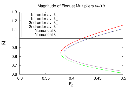
Figure 2: (color online) The magnitude of the Floquet multipliers at $\omega=0.9,\gamma=0.1$. The transition to instability of the dynamics of the parametric oscillator occurs when one of the Floquet multipliers becomes bigger than 1. The second-order averaging prediction [Eq. (47)] of the FMs reproduces very accurately the numerical results. The branching off of the FMs occurs when they become real.

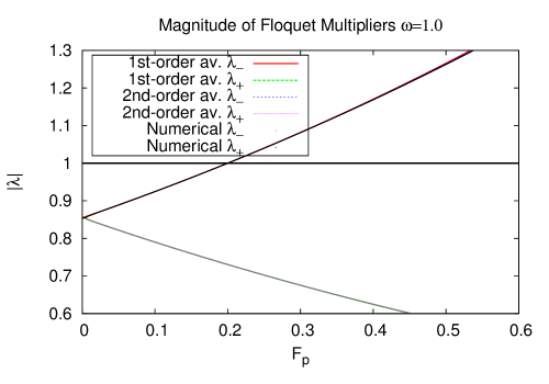
Figure 3: (color online) The magnitude of the Floquet multipliers at $\omega=1.0,\gamma=0.1$. From the onset of the parametric drive the FMs are real. The second-order averaging prediction [Eq. (47)] of the FMs reproduces very accurately the numerical results.

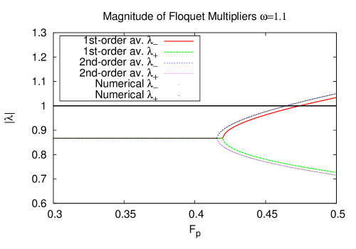
Figure 4: (color online) The magnitude of the Floquet multipliers at $\omega=1.1,\gamma=0.1$. The second-order averaging prediction [Eq. (47)] of the FMs reproduces very accurately the numerical results. Off resonance one notices that the pump amplitude has to be higher before the branching off of the Poincaré map eigenvalues (FMs) in agreement with the results of Fig. (1).

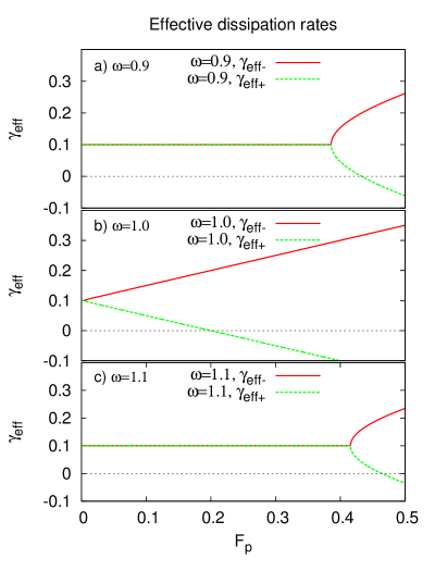
Figure 5: (color online) Effective dissipation rates based on second-order averaging approximation obtained from Eq. (47). Heating and squeezing mostly occur when the floquet multipliers become real and branch off in two different values. Consequently, there is an effective dissipation rate associated with each floquet multiplier. An effective dissipation rate $\gamma_{eff}<\gamma$ cause heating. The different values of $\gamma_{eff}$, one smaller than $\gamma$ and the other larger than $\gamma$, result in squeezing. $\gamma=0.1$

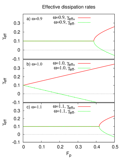
Figure 6: (color online) Numerical effective dissipation rates. Same parameters as in Fig. (5).

In Figs. (2, 3, 4) we show the dependance of the magnitude of the Floquet multipliers (FMs) on the pump amplitude $F_{p}$. When the FMs given by Eq. (47) become real, they branch off in two magnitudes. When this occurs one of the FMs ($\lambda_{-}$) becomes larger as $F_{p}$ is increased, eventually becoming larger than one, when the system given by Eq. (1) becomes unstable, while the other FM ($\lambda_{+}$) becomes smaller. From Eq. (47) this implies into two effective dissipation rates, along the stable manifolds of the Poincaré first-return map (with period $\pi/\omega$, i.e. $\Phi(\pi/\omega)$). This phenomenon causes both heating and squeezing of the parametric oscillator with added noise, since the average power input due to thermal noise remains constant as is shown in Eq. (65) and one effective dissipation rate is decreased. It also causes quadrature thermal squeezing since in one direction, the $\lambda_{-}$-stable manifold of $\Phi(\pi/\omega)$ in the phase space of $u$ and $v$, there is less effective dissipation and, consequently, more fluctuations, while in another direction, the $\lambda_{+}$-stable manifold of $\Phi(\pi/\omega)$ in the phase space of $u$ and $v$, there is more effective dissipation and , consequently, less fluctuations. This inbalance in the effective dissipation rates, we claim, is the main cause of thermal squeezing in the parametric oscillator with added noise. The dependance on pump amplitude of the effective dissipations can be seen on Fig. 5 (second-order averaging result) and on Fig. 6 (Floquet theory numerical result).

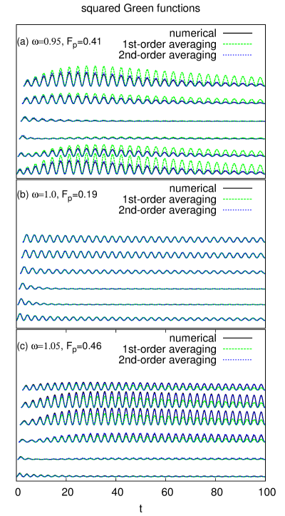
Figure 7: (color online) In the frames above we show several squared Green’s functions with equally-spaced in time initial conditions in one given period of the parametric driving. They are vertically spaced for clarity, since all asymptotes are zero. In each frame we have a comparison between numerical results given by the numerical integration of Eq. (49) and the analytical approximate results given by Eqs. (50) or (52). We have a) $\omega=0.9$, b) $\omega=1.0$, and c) $\omega=1.1$. The initial values of the Green’s functions are $G(t,t^{\prime})=0$ and $\frac{\partial}{\partial t}G(t,t^{\prime})=1.0$ when $t=t^{\prime}+0^{+}$. The pump amplitudes are indicated in the figure frames.

In Fig. 7 we show several squared Green’s functions with initial conditions spread out evenly in time during one period of the pump ($\pi/\omega$). They are vertically spaced only for clarity, since all of their assymptotes are zero. The Green’s functions are shown squared because that is the way they contribute to the thermal fluctuations in Eq. (57). One notices that the second-order approximation Green’s functions yield a much better approximation to the numerical Green’s functions than the first-order approximation. This is specially evidenced the closer one gets to first transition line to instability, a consequence of the fact that the second-order analytical expression for the transition line given in Eq. (48) is a better approximation than the first-order expression in Eq. (25).

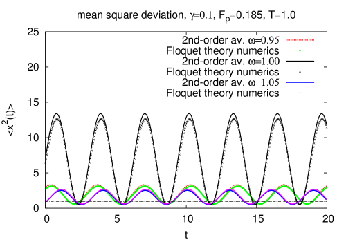
Figure 8: Mean-square deviation $\langle x^{2}(t)\rangle$ time evolution. Comparison between Floquet theory numerical results and second-order averaging results given by Eq. (57) with the Green’s function given by Eq. (52). The dot-long dashed line indicates the temperature of the external heat bath. All pump amplitudes are the same $F_{p}=0.185$. This indicates that the close one is to resonance the larger the squeezing amplitude and average dynamical temperature.

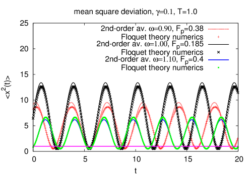
Figure 9: Mean-square deviation $\langle x^{2}(t)\rangle$ time evolution. Comparison between Floquet theory numerical results and second-order averaging results given by Eq. (57) with the Green’s function given by Eq. (52). The dot-long dashed line indicates the temperature of the external heat bath. The values of the pump amplitude were chosen to be close to the transition line given by Eq. (48)

In Fig. 8 we show a comparison between time series of the fluctuation $\langle x^{2}(t)\rangle$ given by Eq. (57) in which the Green’s functions are given either by the second-order approximation expression from Eq. (52) or by the numerical Floquet theory Green’s functions. We use several different Green’s functions with negative detuning ($\omega=0.95$), in resonance ($\omega=1.0$) and positive detuning ($\omega=1.05$) all with the same pump amplitude $F_{p}=0.185$. We observe that the numerical and approximate Green’s functions are very similar and that the squeezing amplitude and heating (proportional to the time average of $\langle x^{2}(t)\rangle$) are very dependant on detuning from resonance. From Fig. 1 one sees that the off resonance results are slightly below the threshold of the strong heating and squeezing zone. In Fig. 9 we show again several time series of the fluctuation $\langle x^{2}(t)\rangle$, but this time the pump amplitudes are chosen such that the parameters are inside the heating zone (as given in Fig. 1) and close to the transition line to instability. One sees then considerably higher dynamical temperatures and squeezing amplitudes for the detuned fluctuations than in the previous figure.

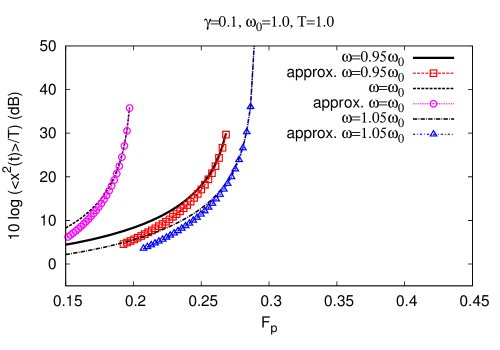
Figure 10: (color online) Log plot of the dc component of the mean square displacement in second-order approximation, $\overline{\langle x^{2}(t)\rangle}$, as given by Eqs. (63). In the parametric oscillator with thermal noise the dynamic temperature of the oscillator grows monotonically until it diverges at the transition line between stable and unstable zones. The simplified approximating curves are given by Eq. (61).

In Fig. 10 we show a logarithmic plot of the dc component of the mean-square displacement over the heat bath temperature. Most of the heating occurs inside the heating zone in which the Floquet multipliers are real, each one with a different amplitude, one that increases and the other that decreases as the pump amplitude is increased.

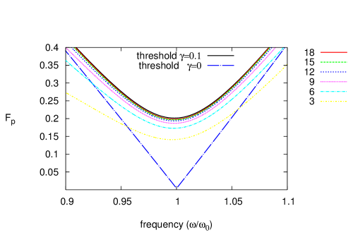
Figure 11: (color online) Countour log plot of dynamic temperatures (the dc component of the statistical average of the square displacement in second-order approximation, $\overline{\langle x^{2}(t)\rangle}$ , as given by Eqs. (63)) over heat bath temperature. Most of the heating occurs inside the heating zone as predicted by our hypothesis. Each level curve is a dynamic isothermal. The levels are given in decibels given by the expression $10\log(\overline{\langle x^{2}(t)\rangle}/T)$, hence each increment of approximately 3 dB increases the dynamic temperature by a factor of 2.

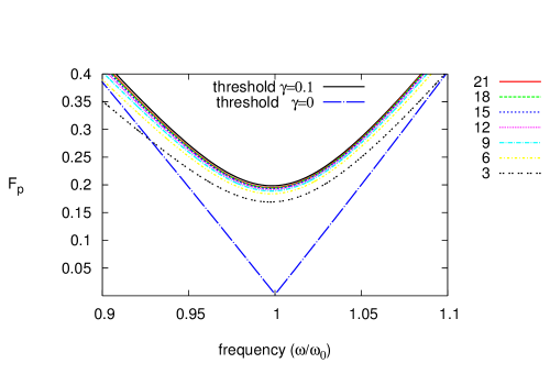
Figure 12: (color online) Countour log plot of the squeezing amplitude (the dc component of the statistical average of the square displacement in second-order approximation, $\sqrt{A_{2\omega}^{2}+B_{2\omega}^{2}}$ , as given by Eqs. (60)) (with the appropriate second-order corrections) over heat bath temperature. Most of the squeezing occurs inside the heating zone as predicted by our hypothesis. Each level curve has constant squeezing amplitude. The levels are given in decibels given by the expression $10\log(\sqrt{A_{2\omega}^{2}+B_{2\omega}^{2}}/T)$.

In Fig. 11 we show level sets in decibels of the dc component of the mean-square displacement over the heat bath temperature in second-order approximation. One sees that most of the heating occurs inside the heating zone in which the Floquet multipliers are real. In Fig. 12 we show level sets of the squeezing amplitude of the mean-square displacement over the heat bath temperature in second-order approximation. This attests that most of the squeezing also occurs inside the heating zone as claimed before.

IV Conclusions

Here, we studied a parametrically-driven oscillator with added noise with the objective of understanding what causes heating and thermal squeezing in the stable zone near the transition line of the first parametric instability. We improved on our previous work batista2011cooling and obtained a more accurate expression for the Green’s functions and, consequently, obtained more precise estimates of the amount of heating and quadrature noise squeezing in the parametrically-driven oscillator. Furthermore, we used an approximate Floquet theory, based on first and second-order averaging approximations, to explain why heating and thermal squeezing occur in the parametrically-driven oscillator with added noise investigated here. These phenomena are related to the onset of real-valued Floquet multipliers (FMs) with different magnitudes. It was shown that as one FM grows while one gets closer (in parameter space) to the first transition line to instability the other FM decreases. As a consequence, one gets two different effective dissipation rates, while at the same time the input power due to noise remains constant as the pump amplitude is increased. We showed that these effects account for most thermal squeezing and heating observed. We showed as well that the second-order Green’s function of the parametric oscillator has the same form as the first-order Green’s function, which implies that with a simple parameter change given in the text all first-order results for the amount of heating and thermal squeezing also apply, with increased accuracy, to second-order approximation. This indicates that a Green’s function renormalization is very well feasible if one goes to higher orders of approximation in the averaging method.

The one-degree of freedom model studied here may be applied for instance to the dynamics of the fundamental mode of an axially loaded doubly-clamped beam resonator. The present model could also be applied to the linear response of ac driven nonlinear oscillators, such as transversally-loaded beam resonators, to noise. We note further that this model can be applied as well to the investigation of the dynamics of ions in quadrupole RF ion guides or traps paul90 in the presence of thermal noise. Most importantly, the notion that we can have two different effective dissipation rates, one for each stable Floquet multiplier, could be used to create control schemes similar to those of the OGY method ott1990controlling to reduce the effects of noise even further in parametric amplifiers and in RF ion traps.

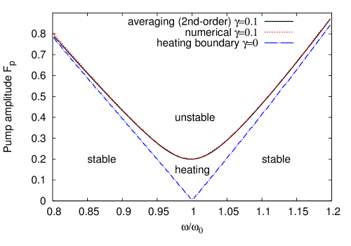
Figure 1: (color online) Comparison between numerical and averaging method predictions for the boundary of the first instability zone of the damped parametrically-driven oscillator of Eq. (1). In the region above the thick solid black line lies the unstable zone obtained by numerical computation, the red dashed line is the second-order averaging prediction [Eq. (48)] for the transition line. The numerical results are obtained by numerically calculating the corresponding Floquet multipliers. The transition line to parametric instability is defined when at least one of them has modulus equal to 1. The heating zone occurs when the Floquet exponents given in Eq. (47) become real. The heating boundary (blue long dashed-dotted line) is equivalent to the transition line to parametric instability when $\gamma=0$.

.

References

• (1) M. Faraday, Philos. Trans. R. Soc. London 121, 319 (1831)
• (2) L. Ruby, Am. J. Phys. 64, 39 (1996)
• (3) W. Mumford, Proceedings of the IRE 48, 848 (1960)
• (4) W. Paul, Rev. of Mod. Phys. 62, 531 (1990)
• (5) M. G. Raizen, J. M. Gilligan, J. C. Bergquist, W. M. Itano, and D. J. Wineland, Phys. Rev. A 45, 6493 (1992)
• (6) M. Drewsen, C. Brodersen, L. Hornekær, J. S. Hangst, and J. P. Schifffer, Phys. Rev. Lett. 81, 2878 (1998)
• (7) D. Kielpinski, C. Monroe, and D. J. Wineland, Nature 417, 709 (2002)
• (8) W. M. Dougherty, K. J. Bruland, J. L. Garbini, and J. Sidles, Meas. Sci. and Technol. 7, 1733 (1996)
• (9) M. Moreno-Moreno, A. Raman, J. Gomez-Herrero, and R. Reifenberger, Appl. Phys. Lett. 88, 193108 (2006)
• (10) M. V. Requa and K. L. Turner, Appl. Phys. Lett. 88, 263508 (2006)
• (11) K. L. Turner, S. A. Miller, P. G. Hartwell, N. C. MacDonald, S. H. Strogatz, and S. G. Adams, Nature 396, 149 (1998)
• (12) B. H. Eom, P. K. Day, H. G. LeDuc and J. Zmuidzinas, Nature Phys. 8, 623–627 (2012)
• (13) A. Szorkovszky, A. C. Doherty, G. I. Harris, and W. P. Bowen, Physical Review Letters 107, 213603 (2011)
• (14) G. Binnig, C. F. Quate, and C. Gerber, Phys. Rev. Lett 56, 930 (1986)
• (15) D. Rugar and P. Grutter, Phys. Rev. Lett. 67, 699 (1991)
• (16) F. DiFilippo, V. Natarajan, K. R. Boyce, and D. E. Pritchard, Phys. Rev. Lett. 68, 2859 (1992)
• (17) V. Natarajan, F. DiFilippo, and D. E. Pritchard, Phys. Rev. Lett. 74, 2855 (1995)
• (18) R. Almog, S. Zaitsev, O. Shtempluck, and E. Buks, Phys. Rev. Lett. 98, 078103 (2007)
• (19) A. A. Batista, J. of Stat. Mech. (Theory and Experiment) 2011, P02007 (2011)
• (20) F. Verhulst, Nonlinear Differential Equations and Dynamical Systems (Springer-Verlag, New York, 1996)
• (21) J. Guckenheimer and P. Holmes, Nonlinear Oscillations, Dynamical Systems, and Bifurcations of Vector Fields (Springer-Verlag, New York, 1983)
• (22) C. Holmes and P. Holmes, J. of Sound and Vib. 78, 161 (1981)
• (23) A. A. Batista, B. Birnir, and M. S. Sherwin, Phys. Rev. B 61, 15108 (2000)
• (24) K. Wiesenfeld and B. McNamara, Phys. Rev. Lett.  55, 13 (1985)
• (25) R. Kubo, Rep. Prog. Phys. 29, 255 (1966)
• (26) A. A. Batista and R. S. N. Moreira, Phys. Rev. E 84, 061121 (2011)
• (27) E. Ott, C. Grebogi, and J. Yorke, Phys. Rev. Lett. 64, 1196 (1990)
Refer to caption