Synchronisation in networks of delay-coupled type-I excitable systems

Abstract

We use a generic model for type-I excitability (known as the SNIPER or SNIC model) to describe the local dynamics of nodes within a network in the presence of non-zero coupling delays. Utilising the method of the Master Stability Function, we investigate the stability of the zero-lag synchronised dynamics of the network nodes and its dependence on the two coupling parameters, namely the coupling strength and delay time. Unlike in the FitzHugh-Nagumo model (a model for type-II excitability), there are parameter ranges where the stability of synchronisation depends on the coupling strength and delay time. One important implication of these results is that there exist complex networks for which the adding of inhibitory links in a small-world fashion may not only lead to a loss of stable synchronisation, but may also restabilise synchronisation or introduce multiple transitions between synchronisation and desynchronisation. To underline the scope of our results, we show using the Stuart-Landau model that such multiple transitions do not only occur in excitable systems, but also in oscillatory ones.

1 Introduction

Studies on complex networks have gained much attention in recent times from various fields of research ALB02a ; NEW03 ; BOC06a . In particular, the dynamics on networks of nonlinear elements (or nodes) has become a very active area TIM02a ; STE06a ; ASH07 ; FLU10b ; LEH11 ; ENG11 ; KAN11 ; OME11 ; DAH12 ; HAG12 ; NEP12 . Here, we consider the dynamics of neurons as a network of nonlinear excitable nodes. While the model we consider is generic for excitability, the local dynamics being modelled in this context is the “firing” mechanism of neurons (i.e. the rise and fall of the electrical membrane potential). This mechanism is the basis for neural coding and information transfer or cell-to-cell communication PER68 . The type of network we primarily focus on in our investigations is the small-world (SW) network WAT98 , which has a short average path distance between nodes, as well as a large degree of clustering (in other words, many triangles in the network structure). These properties are found in many kinds of real-world structures, such as the collaboration between film actors, power grids, the World Wide Web and social relationships WAT98 ; ADA99 ; ALB02a ; NEW03 . In particular, large-scale cortical networks also show these properties SPO00 ; SPO06 . The brain has an architecture enabling both efficient global and local communication between neurons LAT01 , which is captured well by the SW model.

The interest in the synchronisation of neurons emerges from the role it plays in information processing and perception, as well as in epilepsy and similar diseases TRA82 ; ROE97 ; ENG01a ; PIK01 ; MEL07 . While there are several types of synchronisation, the focus here will be on zero-lag synchronisation. This means that the dynamics of all nodes in the network are not only identical but also temporally in-phase.

Inhibition plays an important role in the nervous system HAI06 . Here, when constructing a network we begin with a regular ring network of excitatory links and, as in Ref. LEH11 , we add long-range inhibitory links into the network structure. This creates a SW network of the form proposed in Ref. NEW99b . The introduction of inhibitory links and an increasing of their density in the network was shown in Ref. LEH11 to result in a loss of stable synchronisation.

In this paper, we consider delay-coupled networks of type-I excitability, in contrast to Ref. LEH11 where type-II was considered using FitzHugh-Nagumo local dynamics, and find qualitative differences for a particular range of coupling parameters. The most interesting implication of this is that for some network topologies with this type of excitability increasing the density of inhibitory links may not just lead to one transition from stable to unstable synchronisation, but may lead to multiple transitions. This means that increasing the density of inhibitory links in the network may stabilise synchronisation, rather than destabilise it.

In the following section, we introduce the model and the network topologies considered in the present study. In Sec. 3 we use the master stability function to investigate the stability of arbitrary synchronised networks with given coupling parameters (i.e. the coupling strength and the length of delay between coupled nodes). The master stability function is calculated in Sec. 4 for networks coupled within a range of small delay time and coupling strength, which delivers the main results of the paper - namely, the existence of synchronised states that have different stability conditions compared to coupling with larger delay times. The implications these results may have for specific complex networks are discussed in Sec. 5. In Sec. 6, we study networks of coupled Stuart-Landau oscillators and demonstrate that multiple transitions between synchronisation and desynchronisation can also appear in networks of oscillatory nodes and are not limited to excitable systems.

2 Model

In order to model excitability, the system must have a rest state, which corresponds to a stable fixed point. Small perturbations from the rest state allow for the creation of a large excursion in the phase space, which corresponds to the system entering an excited state before returning to the rest state. In the context of neurodynamics, this is the firing state of the neuron IZH00 .

Neurons can exhibit different excitability properties. In 1948, Hodgkin classified two types of neural excitability HOD48 . Both types can be ordered depending on the type of bifurcations that occurs when the bifurcation parameter is changed such that the system makes a transition from the excitable to the oscillatory regime:

Type-I neurons can generate action potentials of arbitrarily low frequency. This kind of behavior occurs near a saddle-node infinite period (SNIPER) bifurcation, also known as the SNIC bifurcation (saddle-node bifurcation on invariant cycle). The arbitrarily low frequency coincides with the period of the limit cycle going to infinity as the bifurcation parameter approaches a critical value, where the bifurcation occurs.

Type-II neurons are associated with a supercritical Hopf bifurcation. The frequencies of the action potentials lie within a certain non-zero range, while the amplitude of the limit cycle approaches zero with the bifurcation parameter.

As our model for type-I excitability we consider a generic normal-form of a SNIPER bifurcation HU93a ; HIZ07 . This model is mathematically represented by two first-order differential equations:

$$\mathbf{f}(\mathbf{x})=\begin{pmatrix}\dot{x}\\ \dot{y}\end{pmatrix}=\begin{pmatrix}x(1-x^{2}-y^{2})+y(x-b)\\ y(1-x^{2}-y^{2})-x(x-b)\end{pmatrix}.$$ (1)

In polar coordinates $(x=r\cos{\varphi},y=r\sin{\varphi})$ Eq. (1) reads

$$\dot{r} = r\left(1-r^{2}\right)$$ (2)

$$\dot{\varphi} = b-r\cos\varphi.$$ (3)

$b>0$ is the bifurcation parameter. This bifurcation parameter influences the type of dynamics and determines where in the $(x,y)$-plane the fixed points are located, as discussed below.

An important feature that must be taken into account in the mathematical model is that the effect one neuron has on another is not instantaneous. The signals sent between neurons have a finite propagation speed and take a certain time to arrive at the destination neuron, giving rise to a delay time $\tau$.

The dynamics of a network of $N$ elements (labelled $i=1,...,N$) is written:

$$\dot{\mathbf{x}}_{i}=\mathbf{f}(\mathbf{x}_{i})+\sigma\sum_{j=1}^{N}G_{ij}\mathbf{H}(\mathbf{x}_{j}(t-\tau)-\mathbf{x}_{i}(t)),$$ (4)

where $\mathbf{f}(\mathbf{x}_{i})$ is the local dynamics as described by Eq. (1) for each element $\mathbf{x}_{i}=(x_{i},y_{i})$. $G_{ij}$ determines the matrix $\mathbf{G}$ for the network structure, showing which elements are coupling together, and $\mathbf{H}$ is the coupling function. $\mathbf{H}$ is taken to be the $2\times 2$ identity matrix; this means that the $x$-variable at time $t$ is coupled with the $x$-variable at time $t-\tau$, the $y$-variable at time $t$ is coupled with the $y$-variable at time $t-\tau$, but there is no cross-coupling between the $x$- and $y$-variable. The coupling parameters, which are identical for all connections, are the coupling strength $\sigma$ and delay time $\tau$.

For synchronous dynamics, the $2(N-1)$ constraints $\mathbf{x}_{s}\equiv\mathbf{x}_{1}=\mathbf{x}_{2}=\cdots=\mathbf{x}_{N}$ define a 2-dimensional synchronisation manifold (SM) within the $2N$-dimensional phase space and the coupled system is reduced to an effective single system with feedback:

$$\dot{\mathbf{x}}_{s}=\mathbf{f}(\mathbf{x}_{s})+\sigma\mathbf{H}(\mathbf{x}_{s}(t-\tau)-\mathbf{x}_{s}(t)),$$ (5)

with unity row sum $\sum_{j}G_{ij}=1$, so that the nodes all receive the same level of input while they are synchronised. Any non-unity but constant row sum can be rescaled using the coupling strength $\sigma$.

With the bifurcation parameter $b<1$ there exists an unstable focus at the origin, as well as a saddle point and a stable node situated on the unit circle at $(x_{i},y_{i})=(b,\sqrt{1-b^{2}})$ and $(b,-\sqrt{1-b^{2}})$, respectively. At $b=1$ the saddle point and stable node collide, so that for $b>1$ a limit cycle exists along the unit circle. In the case of $b<1$ (excitable regime), a perturbation which pushes the system from the stable node beyond the saddle point can result in a single oscillations along the unit circle. Delayed coupling can induce a homoclinic bifurcation, such that a limit cycle is produced that bypasses the saddle point and stable node HIZ07 ; AUS09 . Here, we will consider the excitable regime with $b=0.95$ and investigate for which topologies the synchronised dynamics of complex networks is stable.

In this paper, two kinds of complex networks are considered: SW networks and Erdős-Rényi random networks ERD59 . We construct the SW networks as a variation to the method proposed in Ref. WAT98 , introduced in Refs. MON99 ; NEW99b : (i) Each of the $N$ nodes in a one-dimensional ring is given excitatory links to its $k$ nearest neighbours on each side. Note that in terms of the matrix $\mathbf{G}$, an excitatory link between the $i^{\textnormal{th}}$ and $j^{\textnormal{th}}$ node means that $G_{ij}>0$, while for an inhibitory link $G_{ij}<0$. (ii) For each of the $kN$ links we add with a probability of $p$ another inhibitory link with strength -1 between two randomly chosen nodes (i.e. on average $pkN$ randomly distributed inhibitory links). (iii) Self-coupling and multiple links between the same two nodes are not allowed. (iv) Finally, the entries in each row of $\mathbf{G}$ are normalised to ensure a unity row sum. If a row sum is equal to zero, then the network realisation is discarded.

The random networks are constructed with $kN$ excitatory links between randomly chosen nodes, as well as $pkN$ randomly distributed inhibitory links, so that these may be compared to a SW network with the same parameters $p$, $k$ and $N$. Because the construction of both kinds of complex networks involves random processes, there will be many possible realisations of either kind of network with a given set of parameters.

In the following, we determine stability of the synchronised dynamics and compare the stability of these different kinds of networks.

3 Stability of Synchronisation

The Master Stability Function (MSF) is a tool that represents a measure of the stability of a synchronised state for given delay-coupling parameters in terms of the topology of an arbitrary network PEC98 . The master stability equation, given by

$$\delta\dot{{\mathbf{x}}}(t)=[D\mathbf{f}(\mathbf{x}_{s})-\sigma\mathbf{H}]\delta{\mathbf{x}}(t)+(\alpha+i\beta)\mathbf{H}\delta{\mathbf{x}}(t-\tau),$$ (6)

is found by linearising Eq. (4) around Eq. (5) and can be used to calculate the largest Lyapunov exponent $\Lambda(\alpha,\beta,\sigma,\tau)$, called the MSF. $\delta{\mathbf{x}}$ is the perturbation of $\mathbf{x}$ away from the SM (i.e. $\mathbf{x}=\mathbf{x}_{s}+\delta\mathbf{x}$) and $D\mathbf{f}(\mathbf{x}_{s})$ is the Jacobian matrix of Eq. (1) evaluated on the SM. Important for this approach is that, whereas one can calculate Lyapunov exponents for a specific network topology using the eigenvalues of the matrix $\mathbf{G}$, one considers here a continuous complex parameter $\alpha+i\beta$ representing the complex plane of possible eigenvalues scaled by the coupling strength $\sigma$ (i.e. $\alpha+i\beta$ is a continuous parametrisation of $\sigma\nu_{j}$, where $\nu_{j}$ are the eigenvalues of $\mathbf{G},j=1,...,N$). Thus, one can calculate the Lyapunov exponents for a region of the $(\alpha,\beta)$-plane which gives sub-regions of stability, where $\Lambda<0$, and instability, where $\Lambda>0$. It is then easy to compare the synchronous stability of various networks by simply observing whether any of their eigenvalues fall inside an unstable region of the $(\alpha,\beta)$-plane. If all the eigenvalues lie within stable regions, then perturbations away from the SM will decay exponentially.

Because of the unity row sum condition, $\mathbf{G}$ always has an eigenvalue $\nu_{1}=1$. This longitudinal eigenvalue (all others are called transversal) corresponds to perturbations within the SM and $\Lambda(\sigma\nu_{1},0,\sigma,\tau)$ is always zero because we are looking at periodic dynamics. As such, it is only the transversal eigenvalues that are important for determining the stability of synchronisation.

Figure 1(a) shows the MSF of the SNIPER model with coupling parameters $\sigma=0.3$ and $\tau=10$. The white dots represent the eigenvalues of the matrix $\mathbf{G}$ for a unidirectional ring of 11 nodes. All eigenvalues are within the stable region of the MSF, thus the synchronisation of all 11 nodes coupled with these parameters is stable.

\begin{overpic}[width=429.28616pt,height=355.57156pt]{Images/blank.jpeg} \put(1.5,45.0){\includegraphics[scale={0.212}]{Images/tau10_sigma3e-1_uniring_N11_compact.pdf}} \put(15.0,76.0){\tiny(a)} \put(0.0,1.0){\includegraphics[scale={0.24}]{Images/tau7_sigma3e-1alpha_compact.pdf}} \put(15.0,38.0){\tiny(b)} \put(51.0,43.8){\includegraphics[scale={0.24}]{Images/tau65e-1_sigma3e-1alpha_compact.pdf}} \put(53.0,76.0){\tiny(c)} \put(51.0,1.0){\includegraphics[scale={0.24}]{Images/tau6_sigma3e-1small_compact.pdf}} \put(53.0,38.0){\tiny(d)} \end{overpic}

Figure 1: (Colour online) Master stability function $\Lambda$ for coupling parameters $\sigma=0.3$ and (a) $\tau=10$, (b) $\tau=7$, (c) $\tau=6.5$, and (d) $\tau=6$. $\alpha$ and $\beta$ are the real and imaginary parts of the scaled eigenvalues of the coupling matrix, $\sigma\nu_{k}$, respectively, and $\Lambda$ is the largest Lyapunov exponent. White dots in panel (a) represent the scaled eigenvalues of a unidirectional ring of 11 nodes ($\sigma\nu_{1},\ldots,\sigma\nu_{11}$). $b=0.95$.

According to Ref. FLU10b , for $\tau$ in the order of the system’s characteristic time scale (in this case, the period of the oscillations) and above, the MSF will always tend towards a rotational symmetry. Examples such as the one above in Fig. 1(a) confirm these general findings for the SNIPER model. When calculating MSFs for a large fixed $\tau$ while varying $\sigma$ it becomes evident that the size of the stable region is scaled by $\sigma$, so that the stable region can be estimated very well by the circle $S((0,0),\sigma)$ (that is, a circle centred at the origin with a radius $\sigma$). Large values of $\tau$, however, despite influencing the Lyapunov exponents quantitatively, do not affect the shape of the stable region.

This rotational symmetry of the MSF was also found for type-II neurons, modelled as FitzHugh-Nagumo oscillators LEH11 . In this case $\sigma$ and $\tau$ do not affect whether the eigenvalues fit into the stable region of the MSF, so that only the topology of a network is important for the stability of its synchronisation. Furthermore, because Gershgorin’s circle theorem GER31 guarantees that the eigenvalues of a network’s coupling matrix with no self-coupling and purely excitatory coupling (i.e. $G_{ii}=0$ and $G_{ij}\geq 0,1\leq i,j\leq N$) lie within the unit circle on the complex plane, the synchronisation of such a network will always be stable. Finally, if additional inhibitory links are introduced with probability $p$ to construct a small-world network as described in Sec. 2, phase transitions from stable to unstable synchronisation are found with increasing probability of inhibition $p$ LEH11 . All these results also apply for the SNIPER neurons with sufficiently large $\tau$.

As an example, Fig. 2 shows the transition from stable synchronisation, where the fraction $f$ of network realisations with unstable synchronisation is zero, to unstable synchronisation, where $f=1$, as the probability of inhibition $p$ is increased. This example is for the coupling parameters $\sigma=0.3$ and $\tau=10$, but this transition to inhibition-induced desynchronization will look the same for all sufficiently large values of $\tau$. A thorough investigation of the effects of additional inhibitory links when $\tau$ is small will be presented in Sec. 5.

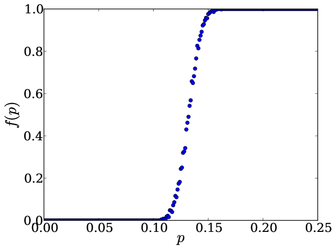
Figure 2: (Colour online) Fraction of desynchronised networks $f(p)$ vs. probability of inhibitory links $p$ for 100 realisations of SW networks of $N=100$ and $k=24$ for $\sigma=0.3$, $\tau=10$, $b=0.95$.

4 Small delay times

If the delay time is not large enough, the rotational symmetry of the MSF no longer holds. In fact, while reducing $\tau$ one can witness how the rotational symmetry begins to break down. This is depicted in Fig. 1. For a constant coupling strength of $\sigma=0.3$, the MSFs are numerically calculated for decreasing delay times. While at $\tau=10$ the MSF still has its circular form (Fig. 1(a)), when decreasing $\tau$, the stable (i.e. dark blue/green) region of the MSF begins to show signs of deformation. By $\tau=7$ (see Fig. 1(b)) the stable region is clearly larger than the unit circle scaled by $\sigma=0.3$ and has definitely lost its rotational symmetry. By $\tau=6.5$ (see Fig. 1(c)) the stable region has already split into two disconnected regions. Letting $\tau$ decrease further, the stable regions become increasingly smaller (see Fig. 1(d)). Note that the delay-induced limit cycle coexists alongside the stable fixed point and whether it is reached or not is therefore dependent on initial conditions. For $\tau$ less than about 4 (not shown here), the coupling is no longer able to induce the homoclinic bifurcation that creates the limit cycle at all (as discussed in Sec. 2), in other words, the neurons no longer oscillate. Instead, all solutions approach the stable fixed point.

It is now obvious that, in this regime of small delay, small changes in $\tau$ can have a great impact on the stability. Despite the seemingly sudden change in the MSFs in Fig. 1 between $\tau=7$ and $\tau=6.5$, the evolution of the boundary of stability is in fact a continuous one (except at a critical value $\tau_{c}$, which will be discussed below). This becomes clear after plotting the MSF versus the real part $\alpha$ of the eigenvalue (with $\beta=0$) for varying $\tau$. Taking this one slice of the eigenvalue plane gives a good indication of the growth and decay of the stable region in the MSF while changing $\tau$. Figure 3 shows the MSF as a function of the real part $\alpha$ ($\beta=0$) and the delay time $\tau$, with fixed coupling strengths of (a) 0.25, (b) 0.30 and (c) 0.35. This produces an MSF on an $(\alpha,\tau)$-plane, which can be used for network topologies with a coupling matrix that yields real eigenvalues, e.g. symmetric matrices for undirected networks. In the following we restrict ourselves to undirected networks.

\begin{overpic}[width=390.25534pt]{Images/tau46e-1-12_sigma25e-2_alpha_tau_c.pdf} \put(14.0,66.0){\small(a)} \end{overpic}

\begin{overpic}[width=390.25534pt]{Images/tau4-10_sigma3e-1_alpha_tau_c.pdf} \put(12.0,68.0){\small(b)} \end{overpic}

\begin{overpic}[width=390.25534pt]{Images/tau45e-1-10_sigma35e-2_alpha_tau_c.pdf} \put(12.0,68.0){\small(c)} \end{overpic}

Figure 3: (Colour online) MSF $\Lambda$ for a fixed coupling strength (a) $\sigma=0.25$, (b) $\sigma=0.3$ and (c) $\sigma=0.35$ in the plane of the real part $\alpha$ ($\beta=0$) and the delay time $\tau$. The horizontal red lines show the position of the critical delay time $\tau_{c}$. $b=0.95$.

Based on the exemplary coupling strengths in Fig. 3 it is clear that the stability depends on both $\sigma$ and $\tau$. In all examples the vertical boundary line at $\alpha=\sigma$, corresponding to the longitudinal eigenvalue (i.e. $\nu_{0}=1$, where $\Lambda=0$), can be easily identified. It separates regimes of stable and unstable synchronisation. Another common characteristic is that the $\tau$-dependent MSFs have a critical delay time $\tau_{c}$ at which the stable region splits into two separate, disconnected regions. For values above $\tau_{c}$ the stable region is found to the left of the longitudinal eigenvalue; whereas for values below $\tau_{c}$ there may be one stable region to the right of the longitudinal eigenvalue and one to the left. $\tau_{c}$ seems to be an important value, because it marks the most significant $\tau$-dependent qualitative change in the MSF. Ultimately, the MSF can be divided into three regimes of $\tau$: (i) two or more smaller separate regions of stability exist when $\tau<\tau_{c}$; (ii) one large region of stability exists when $\tau>\tau_{c}$; (iii) the MSF has one rotationally symmetric region of stability in the limit of $\tau\rightarrow\infty$ (which holds already in good approximation if $\tau$ is of the order of the intrinsic oscillation period or larger).

Clearly, the topological criteria for stable synchronisation will be very different depending on whether the network is coupled with $\tau<\tau_{c}$ or $\tau>\tau_{c}$. Observing the change in the limit cycles while varying $\tau$ offers the explanation for the qualitative change either side of $\tau_{c}$ in the MSF. For smaller $\tau$ values, the trajectory of the limit cycle is sensitive to changes in the coupling parameters, whereas, for larger $\tau$ values, the trajectory changes very gradually and approaches an elliptical form. The most predominant feature of the changing limit cycle is a large “kink” for values below $\tau_{c}$. Figure 4(a) shows such a kink in the limit cycle induced by the coupling parameters $\sigma=0.35$ and $\tau=5.35$: upon bypassing the stable node the limit cycle deviates a little towards the unstable focus, located at the origin, before suddenly changing its trajectory back towards the saddle point. The kink has a large effect on the dynamics of synchronised nodes and is an important source of instability. Simulations have shown that it is at the kink that synchronised nodes begin to diverge from one another following any small perturbations. For larger $\tau$ the kink diminishes and disappears (see Fig. 4(b)).

\begin{overpic}[width=228.08453pt]{Images/tau535e-2_sigma35e-2_vectors_j00003400.pdf} \put(24.0,74.0){\small(a)} \end{overpic}

\begin{overpic}[width=196.86119pt]{Images/tau6_sigma35e-2_vectors_j00002640_noy.pdf} \put(12.0,85.0){\small(b)} \end{overpic}

Figure 4: (Colour online) The position in phase space of one element representing the synchronised dynamics of a network (large green diamond) is shown relative to its delayed position (small green diamond). The black circle and the white circle represent the stable and saddle point, respectively. For small delay times such as (a) $\tau=5.35$ a kink may be the result of the relative positioning. For larger delay times such as (b) $\tau=6$ this does not occur. The movement of the phase point has a local component (dark green arrow) and a coupling component (light green arrow). The coupling component is directed towards the phase point at time $t-\tau$ (small green circle). $\sigma=0.35$, $b=0.95$.

Let us explain the cause for the kink in greater detail. The large green diamond in Fig. 4(a) is the position of a node that represents the dynamics of a synchronised network in the phase space. The small green diamond is its delayed phase point, to which it is coupled, and represents the delayed dynamics of the same synchronised network (i.e. the small green diamond at time $t$ is the large green diamond at time $t-\tau$). A node coupled with a delayed node is attracted towards the direction of this delayed node (cf. Fig. 4(b)). As the node passes between the stable fixed point and the saddle point, it is slowed down, allowing its delayed node to “catch up” to it. For smaller $\tau$ this has the effect that the node is attracted in a clockwise direction towards its delayed node and gets slowed down (cf. Fig. 4(a)). This is the cause for the kink. Whereas for larger $\tau$, the (small green) delayed node is always more than half a rotation behind, meaning that the (large green) node is attracted towards it in an anti-clockwise direction. This gives the limit cycle a form that is roughly circular as seen in Fig. 4(b).

As long as the kink is present in the limit cycle, a synchronised network will generally have very different topological conditions in order to be stable. Even when the limit cycle has a very predominant (sharp) kink, it will often be possible to find a class of networks that will still show stable synchronisation.

Note that in Fig. 3 one can see how the most stable part of the stable region (i.e. where $\Lambda$ is at its smallest) shifts away from $\alpha=0$ as $\tau$ becomes smaller. Simulations have shown that this happens while the angle of the kink increases (making the kink “sharper”). A possible interpretation could be as follows. Each potential eigenvalue of the coupling matrix in a MSF is associated with one or more eigenvectors in the $N$-dimensional space. These eigenvectors are all orthogonal to the vector $(1,1,1,...,1)$ that represents motion in the SM. This would suggest that the increasing angle of the kink corresponds to a shifting of the most stable direction of perturbation transverse to the SM.

5 Implications for complex networks with a small delay coupling time

An obvious observation is that networks with purely excitatory coupling, which are always stable for large delay times as mentioned at the end of Sec. 3, may not show stable synchronisation for $\tau<\tau_{c}$. It was explained in Sec. 3 that increasing the probability $p$ of inhibitory links in the network can be a factor leading to unstable synchronisation. This occurs because a larger probability of inhibition can push a part of the eigenvalue spectrum of any network beyond the longitudinal eigenvalue at $\alpha=\sigma$ (because Gershgorin’s circle theorem no longer holds) and into the unstable region of the MSF. Now, for smaller $\tau$, there may be a pocket of stability to the right of the longitudinal eigenvalue, so that increasing inhibition can make the otherwise unstable synchronisation of a network stable.

This means that the transitions between stable and unstable synchronisation as a function of the probability of inhibition $p$ discussed in Ref. LEH11 are no longer valid when $\tau$ is small. The transitions are now sensitive to the coupling parameters, not just the network parameters $N$ and $k$. Due to the multiple regions of stability, eigenvalues may wander in and out of stable regions, while increasing the probability of inhibition $p$. For large $\tau$, increasing $p$ in the SW network model only results in one transition where the fraction of desynchronising networks (i.e. networks with unstable synchronisation) $f(p)$ switches from 0 to 1 (cf. Fig. 2). For small $\tau$, it is possible that $f(p)$ jumps back to 0, before increasing again to 1. This will occur if there is a separate region of stability to the right side in the MSF that is large enough that all the eigenvalues lying over there can fit inside.

The observation of multiple transitions between stable and unstable synchronisation can be explained by looking at the eigenvalue spectra for SW networks for various $p$ values. As discussed above in relation to the MSF method, each network topology has a coupling matrix $\mathbf{G}$, the eigenvalues from which can be used to determine the stability of the network’s synchronised state. Because the “short-cuts” in the SW network are randomly introduced, each network with specific $N$, $k$ and $p$ values may have many realisations. By calculating the eigenvalues for a large number of realisations of the SW network with certain parameters (i.e. given $N$, $k$ and $p$), one can find the bounds for the eigenvalue spectra.

Figure 5 displays the superimposed eigenvalue spectra of 500 realisations for SW networks with parameters $N=200$ and $k=20$ (regular ring with excitatory coupling of $k$ nearest neighbours on either side) in dependence on the probability of inhibition $p$. The longitudinal eigenvalues located at $\nu_{1}=1$ have been removed. One can see that the bounds for possible eigenvalues shift depending on the value of $p$. One can also see how the spectra begin to increasingly resemble the semicircular distribution ALB02a of a random network for larger $p$ values, where the networks have lost their SW properties.

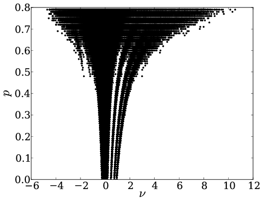
Figure 5: Spectra of eigenvalues $\nu$ of undirected small world networks with $N=200$ and $k=20$ and varying probability $p$ of inhibitory links. 500 realisations of the eigenvalue spectrum are plotted for each value of $p$.

The eigenvalue spectra bridge the gap between observations of the MSF (i.e. the dependence of the stability of synchronisation on the eigenvalues) and what is seen in these transitions (i.e. the dependence of stability on the network topology). Increasing $p$ allows isolated eigenvalues to increase in value and, in terms of the MSF, shift their locations further to the right in the $(\alpha,\beta)$-plane. This is visualised in Fig. 6. Figures 6(b), (d) and (f) show the eigenvalue spectra for SW networks with $N=200$ elements and $k=40$, 20, and 50, respectively.

\begin{overpic}[width=143.09538pt]{Images/trans_N200_k40_small.jpg} \put(18.0,65.0){\tiny(a)} \end{overpic}

\begin{overpic}[width=143.09538pt]{Images/trans_N200_k20_small.jpg} \put(18.0,65.0){\tiny(c)} \end{overpic}

\begin{overpic}[width=143.09538pt]{Images/trans_N200_k50_small.jpg} \put(18.0,65.0){\tiny(e)} \end{overpic}

\begin{overpic}[width=143.09538pt]{Images/eigenvalues_N200_k40_small_p0-5e-1_tau65e-1_sigma3e-1.jpg} \put(18.0,65.0){\tiny(b)} \end{overpic}

\begin{overpic}[width=143.09538pt]{Images/eigenvalues_N200_k20_small_p0-5e-1_tau65e-1_sigma3e-1.jpg} \put(18.0,65.0){\tiny(d)} \end{overpic}

\begin{overpic}[width=143.09538pt]{Images/eigenvalues_N200_k50_small_p0-5e-1_tau65e-1_sigma3e-1.jpg} \put(18.0,65.0){\tiny(f)} \end{overpic}

Figure 6: (Colour online) Fraction of desynchronized networks $f$ in dependence of the probability of additional inhibitory links $p$ for 500 realisations of networks of $N=200$ with (a) $k=40$, (c) $k=20$, and (e) $k=50$ with $\sigma=0.3$ and $\tau=6.5$. Corresponding eigenvalue spectra for (b) $k=40$, (d) $k=20$, and (f) $k=50$ with $100$ realisations for each $p$ value. Here the green shaded regions represent the stable regions of the real part of the MSF. $b=0.95$.

Figures 6(a), (c) and (e) show the corresponding fraction of desynchronised networks $f$ in dependence on the probability of additional inhibitory links $p$. Consider, for instance, SW networks with parameters $N=200$ and $k=40$. In Fig. 6(a) $f(p)$ is shown for the exemplary coupling parameters $\sigma=0.3$ and $\tau=6.5$ with a corresponding plot of eigenvalues in Fig. 6(b). Note that the grey (green) shaded regions represent the stable regions of the line $\beta=0$ on the $(\alpha,\beta)$-plane of the MSF for $\sigma=0.3$ and $\tau=6.5$ (cf. Fig. 1(c)). For coupling parameters where this region of stability is not large enough, $f$ may briefly dip below $1$ without decreasing to $0$, because only some realisations may have eigenvalues that fit inside the stable region. In Fig. 6(c) where $k=20$, $f$ dips down to $0.14$, because at most $14\%$ of the realisations show stable synchronisation (i.e. all the eigenvalues are inside the stable region). If the distance between the larger isolated eigenvalues matches the distance between stable regions (which is almost the case in Fig. 6(d)), then the transition curve only just touches the $f=0$ axis at some value of $p$ before increasing back to $f=1$. Figure 6(e) is an example where a further transition is possible, because not only do all eigenvalues begin in stable regions at $p=0$, but there is another regime of $p$ where all eigenvalues fit inside stable regions. Note that the length of the transition from $f=0$ to $f=1$ is actually a measure of the variance of the isolated eigenvalues for an ensemble of realisations. For example, the variance of the isolated eigenvalues decreases as $N$ is increased, so that the length of transition will be shorter in larger networks, and the transition becomes sharper.

When constructing a histogram of the eigenspectra for a particular value of $p$ – see Fig 7(a) – the larger isolated eigenvalues seen to the right, e.g. in Fig. 6(d), result in small peaks of eigenvalues.

\begin{overpic}[width=212.47617pt]{Images/eig_spectrum_N100_k10_2e-1_small.pdf} \put(0.0,68.0){\tiny(a)} \end{overpic}

\begin{overpic}[width=212.47617pt]{Images/eig_spectrum_N100_k10_2e-1_random.pdf} \put(0.0,68.0){\tiny(b)} \end{overpic}

Figure 7: Histograms of eigenvalue spectra for $1000$ realisations of (a) SW networks and (b) random networks with the same number of nodes, the same number of excitatory links and the same probability of inhibitory links. $N=100$, $k=10$, $p=0.2$ and number of bins is $1000$.

For each realisation of many SW networks there are isolated eigenvalues that are larger than most other eigenvalues in the spectrum. The small peaks of eigenvalues result from perturbations in isolated eigenvalues. The spectrum of a regular ring network (i.e. a SW network with $p=0$) can be found analytically using the graph’s symmetry operations FAR01 and is given by

$$\nu_{l} = \frac{1}{k}\sum\limits_{j=1}^{k}\cos\left(2\pi j\frac{l}{N}\right)$$ (7)

$$= \frac{1}{k}\left(\frac{\cos\left(k\pi\frac{l}{N}\right)\sin\left((k+1)\pi\frac{l}{N}\right)}{\sin\left(\pi\frac{l}{N}\right)}-1\right),$$

where $l=1,...,N-1$. Figure 8 shows this eigenspectrum for the $p=0$ case.

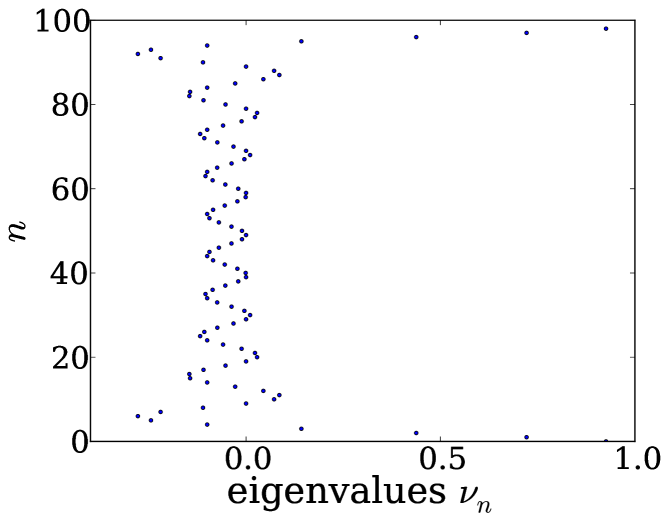
Figure 8: The eigenvalue spectrum for a regular network with $N=100$ and $k=10$. $\nu_{n}$ is the value of the $n^{th}$ eigenvalue.

As $p$ is increased these eigenvalues will be slightly perturbed (in a random manner) by the changing network structure, of which many realisations are possible. In Fig. 8 one can see the isolated eigenvalues to the right-hand side of the plot that eventually evolve into the smaller side peaks of eigenvalues in histograms for larger $p$ (see Fig 7(a)). These peaks show the distribution of the eigenvalue under the influence of the random nature of the SW “short-cuts” creation process – which is why the smaller eigenvalue peaks can be approximated by a normal distribution . This is furthermore the reason why the desynchronisation transitions observed in Ref. LEH11 and Figs. 6(a), (c) and (e) look like the cumulative (integrated) distribution function. They reflect how increasing $p$ brings the area of the small eigenvalue peak accumulatively into the unstable region of the MSF.

To explain why the peaks wander with increasing $p$, consider not normalising the rows of matrix $\mathbf{G}$, so that the row sums are not necessarily equal to $1$. Then the location of the longitudinal eigenvalue decreases with $p$, because it is equal to the average row sum of $\mathbf{G}$ which is equal to $2k(1-p)$. The locations of the other peaks increase slightly to maintain the eigenvalue sum of zero (a result of the trace of $\mathbf{G}$ being zero, since there is no self-feedback coupling), although for large $N$ this has only a small effect. Thus, scaling the eigenvalues so that the longitudinal eigenvalue is always at $1$ means that the transversal eigenvalues are multiplied by $\frac{1}{2k(1-p)}$, so that they appear to increase with $p$, as seen in Figs. 6(b), (d) and (f).

The case of random Erdős-Rényi networks ERD59 is different. At $p=0$ there are no larger gaps between the eigenvalues, such as those for SW networks at $p=0$. If a random network is fully connected (i.e. is one single component) then the distribution of its eigenvalues at $p=0$ are confined to a semi-circle, given by the semicircular distribution

$$\rho(\nu)=\begin{cases}\frac{\sqrt{4Nq(1-q)-[\frac{\nu}{q(N-1)}]^{2}}}{2\pi Nq(1-q)}&\textnormal{if }\|\nu\|<2\frac{\sqrt{Nq(1-q)}}{q(N-1)}\\ 0&\textnormal{otherwise},\end{cases}$$ (8)

where $q$ is the probability of excitatory links ALB02a . While there are initially no gaps in the eigenvalue distribution at $p=0$, adding inhibitory links to the network (i.e. increasing $p$) does not lead to the creation of any gaps like those seen for SW networks. To illustrate this point, Fig. 7(b) shows the eigenvalue distribution for many realisations of Erdős-Rényi random networks with the same number of nodes, as well as the same number of excitatory links and the same probability of inhibitory links. As a result, multiple transitions between stable and unstable synchronisation will not occur.

One can, however, use Eq. (8) to find parameters $N$ and $q$ such that the eigenvalue distribution is confined to a stable region of the MSF at $p=0$, as long as there is a stable region centred around $\nu=0$ (for example, see Fig. 1(c)). This allows for a desynchronisation transition with increasing $p$, such as in Fig. 2.

6 Small-world networks of Stuart-Landau oscillators

The appearance of multiple transitions between synchronisation and desynchronisation is based on the interplay of the peculiar spectral properties of the small-world topology and the unconnected stable regions that show up in the MSF for the excitable SNIPER model for small delay times.

In this Section we show that such unconnected stable regions may also appear in the MSF of a purely oscillatory system. We consider the Stuart-Landau oscillator, which is the normal form of any oscillatory system near a supercritical Hopf bifurcation. The dynamics of the Stuart-Landau oscillator is governed by a complex variable $z\in\mathbb{C}$, such that we have $\mathbf{x}_{i}=z_{i}$ in Eq. (4). The local dynamics of the Stuart-Landau oscillator is given by

$$f(z)=(\lambda+i\omega-\left|z\right|^{2})z.$$ (9)

For $\lambda>0$, the uncoupled system exhibits self-sustained limit cycle oscillations with radius $r_{0}=\sqrt{\lambda}$ and frequency $\omega$. The coupled system shows – depending on coupling parameters and topology – a variety of synchronised and desynchronised solutions, including amplitude death and cluster synchronisation CHO09 ; CHO11 .

Here we focus on complete (zero-lag) synchronization.

\begin{overpic}[width=199.4681pt]{sachin/fig1_1.pdf} \put(25.0,58.0){\tiny(a)} \end{overpic}

\begin{overpic}[width=199.4681pt]{Images/trans_N200_k40_small_STU.jpg} \put(18.0,65.0){\tiny(c)} \end{overpic}

\begin{overpic}[width=199.4681pt]{sachin/fig3_1a.pdf} \put(15.0,63.0){\tiny(b)} \end{overpic}

\begin{overpic}[width=199.4681pt]{Images/eigenvalues_N200_k40_small_p0-5e-1_STU_tau15e-1pi_sigma8e-2} \put(18.0,65.0){\tiny(d)} \end{overpic}

Figure 9: (Colour online) Network of Stuart-Landau oscillators according to Eqs. (4) and (9): (a) MSF in the $(\alpha,\beta)$ plane for $\tau=3\pi/2$. (b) MSF in the $(\alpha,\tau)$ plane for $\beta=0$. (c) Fraction of desynchronized networks $f$ in dependence of the probability of additional inhibitory links $p$ for 500 realisations of networks of $N=200$ and $k=40$, $\tau=3\pi/2$. (d) Corresponding eigenvalue spectra, where the green shaded areas represent stable regions. Other parameters: $\lambda=0.1$, $\omega=1$, $\sigma=0.08$.

Fig. 9(a) shows the MSF for sets of parameters that allow for unconnected stable regions in the complex plane of the eigenvalues $(\alpha,\beta)$. As shown in Fig. 9(b) a connected stability region occurs for integer multiples of $\tau=2\pi/\omega=2\pi$, while unconnected stability regions – which can lead to multiple phase transitions in SW networks – occur in between.

For the parameters used in Fig. 9(a), Fig. 9(c) shows the fraction of desynchronised networks for the modified small-world model as in Sec. 5. Figure 9(d) shows the eigenspectra for networks of $N=200$ elements, starting from a one-dimensional ring with excitatory coupling to $k=40$ neighbours to either side. Increasing the probability of additional inhibitory links $p$ broadens the spectra and leads to a second regime of stable synchronisation matching the transitions in Fig. 9(c).

7 Conclusion

We have investigated transitions between synchronisation and desynchronisation in complex networks of delay-coupled excitable elements of type I, induced by varying the balance between excitatory and inhibitory couplings in a small-world topology. In our analysis we have used the master stability function approach. For large delay times it seems that both type-I neurons, as modelled here, and type-II neurons, as modelled in Ref. LEH11 , must fulfill similar topological conditions in the network to allow for a stable synchronised state. This is different when considering small delay times. For a range of small coupling strengths and small delay times we have found novel multiple transitions between synchronisation and desynchronisation, when the fraction of inhibitory links is increased. Unlike the Erdős-Rényi random network, a small world model for complex networks with regular excitatory couplings and random inhibitory shortcuts has eigenvalue spectra with gaps between the larger eigenvalues, so that histograms of many realisations reveal isolated peaks of possible eigenvalues. It was shown that, because of this, synchronised small world networks can go through multiple transitions of stability in dependence on the probability of inhibitory short-cuts. Our results are valid beyond the special model of type-I excitability, as we have demonstrated using the Stuart-Landau oscillator.

This work was supported by the DFG in the framework of the SFB 910. PH acknowledges support by the BMBF (grant no. 01GQ1001B).

References

- (1) R. Albert, A.L. Barabási, Rev. Mod. Phys. 74, 47 (2002)
- (2) M.E.J. Newman, SIAM Review 45, 167 (2003)
- (3) S. Boccaletti, V. Latora, Y. Moreno, M. Chavez, D.U. Hwang, Physics Reports 424, 175 (2006)
- (4) M. Timme, F. Wolf, T. Geisel, Phys. Rev. Lett. 89, 258701 (2002)
- (5) A.J. Steele, M. Tinsley, K. Showalter, Chaos 16, 015110 (2006)
- (6) P. Ashwin, G. Orosz, J. Wordsworth, S. Townley, SIAM J. Appl. Dyn. Syst. 6, 728 (2007)
- (7) V. Flunkert, S. Yanchuk, T. Dahms, E. Schöll, Phys. Rev. Lett. 105, 254101 (2010)
- (8) J. Lehnert, T. Dahms, P. Hövel, E. Schöll, Europhys. Lett. 96, 60013 (2011)
- (9) A. Englert, S. Heiligenthal, W. Kinzel, I. Kanter, Phys. Rev. E 83, 046222 (2011)
- (10) I. Kanter, M. Zigzag, A. Englert, F. Geissler, W. Kinzel, Europhys. Lett. 93, 60003 (2011)
- (11) I. Omelchenko, Y.L. Maistrenko, P. Hövel, E. Schöll, Phys. Rev. Lett. 106, 234102 (2011)
- (12) T. Dahms, J. Lehnert, E. Schöll, Phys. Rev. E 86, 016202 (2012)
- (13) A. Hagerstrom, T.E. Murphy, R. Roy, P. Hövel, I. Omelchenko, E. Schöll, Nature Physics 8, 658 (2012), published online
- (14) T. Nepusz, T. Vicsek, Nature Physics 8, 568 (2012)
- (15) D.H. Perkel, T.H. Bullock, Neurosci Res Program Bull 6, 221 (1968)
- (16) D.J. Watts, S.H. Strogatz, Nature 393, 440 (1998)
- (17) L.A. Adamic, The Small World Web, Vol. 1696/1999 of Lecture Notes in Computer Science (Springer Berlin / Heidelberg, 1999), ISBN 978-3-540-66558-8
- (18) O. Sporns, G. Tononi, G.M. Edelman, Cereb. Cortex 10, 127 (2000)
- (19) O. Sporns, Biosystems 85, 55 (2006)
- (20) V. Latora, M. Marchiori, Phys. Rev. Lett. 87, 198701 (2001)
- (21) R.D. Traub, R.K. Wong, Science 216, 745 (1982)
- (22) P. Roelfsema, A. Engel, P. K nig, W. Singer, Nature 385, 157 (1997)
- (23) A. Engel, P. Fries, W. Singer, Nature Reviews Neuroscience 2, 704 (2001)
- (24) A.S. Pikovsky, M.G. Rosenblum, J. Kurths, Synchronization, A Universal Concept in Nonlinear Sciences (Cambridge University Press, Cambridge, 2001)
- (25) L. Melloni, C. Molina, M. Pena, D. Torres, W. Singer, E. Rodriguez, J. Neurosci. 27, 2858 (2007)
- (26) B. Haider, A. Duque, A.R. Hasenstaub, D.A. McCormick, J. Neurosci. 26, 4535 (2006)
- (27) M.E.J. Newman, D.J. Watts, Phys. Lett. A 263, 341 (1999)
- (28) E.M. Izhikevich, Int. J. Bifurcation Chaos 10, 1171 (2000)
- (29) A.L. Hodgkin, J. Physiol. 107, 165 (1948)
- (30) G. Hu, T. Ditzinger, C.Z. Ning, H. Haken, Phys. Rev. Lett. 71, 807 (1993)
- (31) J. Hizanidis, R. Aust, E. Schöll, Int. J. Bifur. Chaos 18, 1759 (2008)
- (32) R. Aust, P. Hövel, J. Hizanidis, E. Schöll, Eur. Phys. J. ST 187, 77 (2010)
- (33) P. Erdős, A. Rényi, Publ. Math. Debrecen 6, 290 (1959)
- (34) R. Monasson, Eur. Phys. J. B 12, 555 (1999)
- (35) L.M. Pecora, T.L. Carroll, Phys. Rev. Lett. 80, 2109 (1998)
- (36) S.A. Gerschgorin, Izv. Akad. Nauk. SSSR 7, 749 (1931)
- (37) I. Farkas, I. Derenyi, A.L. Barabási, T. Vicsek, Phys. Rev. E 64, 026704 (2001)
- (38) C.U. Choe, T. Dahms, P. Hövel, E. Schöll, Phys. Rev. E 81, 025205(R) (2010)
- (39) C.U. Choe, T. Dahms, P. Hövel, E. Schöll, Control of synchrony by delay coupling in complex networks, in Proceedings of the Eighth AIMS International Conference on Dynamical Systems, Differential Equations and Applications (American Institute of Mathematical Sciences, Springfield, MO, USA, 2011), pp. 292–301, DCDS Supplement Sept. 2011