Interpretation of the Veiling of the Photospheric Spectrum for T Tauri Stars in Terms of an Accretion Model.

PACS numbers: 97.10.Ex; 97.10.Qh; 97.21.+a

Keywords: stars – individual: RU Lup, S CrA NW, S CrA SE, DR Tau, RW Aur – T Tauri stars – stellar atmospheres – radiative transfer – spectra.

Abstract

The problem on heating the atmospheres of T Tauri stars by radiation from an accretion shock has been solved. The structure and radiation spectrum of the emerging so-called hot spot have been calculated in the LTE approximation. The emission not only in continuum but also in lines has been taken into account for the first time when calculating the spot spectrum. Comparison with observations has shown that the strongest of these lines manifest themselves as narrow components of helium and metal emission lines, while the weaker ones decrease significantly the depth of photospheric absorption lines, although until now, this effect has been thought to be due to the emission continuum alone. The veiling by lines changes the depth of different photospheric lines to a very different degree even within a narrow spectral range. Therefore, the nonmonotonic wavelength dependence of the degree of veiling $r$ found for some CTTS does not suggest a nontrivial spectral energy distribution of the veiling continuum. In general, it makes sense to specify the degree of veiling $r$ only by providing the set of photospheric lines from which this quantity was determined. We show that taking into account the contribution of lines to the veiling of the photospheric spectrum can cause the existing estimates of the accretion rate onto T Tauri stars to decrease by several times, with this being also true for stars with a comparatively weakly veiled spectrum. Neglecting the contribution of lines to the veiling can also lead to appreciable errors in determining the effective temperature, interstellar extinction, radial velocity, and $v\,\sin i.$

Introduction

Long ago Joy (1949) noticed that the depths and equivalent widths of photospheric lines in the spectra of T Tauri stars were smaller than those for main-sequence stars of the same spectral types, especially at short wavelengths. This effect is commonly explained by the fact that the absorption lines of the stellar photosphere are ”veiled” by the emission continuum, the understanding about the nature of which changed as the views of the cause of activity in T Tauri stars changed.

The emission in optical lines and continuum as well as the very intense ultraviolet (UV) and X-ray emissions had long been thought to be due to the existence of thick chromospheres and coronas around young $(t<10^{7}$ yr) low-mass $(M<2\,M_{\odot})$ stars that to some extent are analogous to the solar ones (see the reviews by Bertout (1989) and references therein). However, it had become clear by the early 1990s that this explanation is appropriate only for moderately active young stars in the spectra of which the equivalent width $(EW)$ of the $H_{\alpha}$ emission line does not exceed 5-10 Å  there is virtually no veiling. Below, we will not talk about these objects called weak-lined T Tauri stars.

Here, we will deal with the so-called classical T Tauri stars $(EW_{H\alpha}>10$ Å). Their observed manifestations can be explained in terms of the model of mass accretion from a protoplanetary disk onto a young star that has a global magnetic field with a strength $\sim 1-3$ kG. The model suggests that the matter from the inner disk is frozen in the magnetic field lines and slides down toward the star along them, being accelerated by gravity to a velocity $V_{0}\sim 300$ km s^-1. A shock wave at the front of which the gas velocity decreases approximately by a factor of 4 and the gas is abruptly heated to a temperature of $\sim 10^{6}$ K emerges near the stellar surface. The postshock matter cools down while gradually radiating its thermal energy in the UV and X-ray ranges and settles to the stellar surface while reducing its velocity.

One half of the short-wavelength radiation flux of the shock from the cooling zone escapes upward, heating and ionizing the pre-shock gas, and the second half irradiates the star, producing the so-called hot spot on its surface. Estimations (Königl 1991; Lamzin 1995) and numerical calculations (Calvet and Gullbring 1998) show that for classical T Tauri stars (CTTS) at a particle number density in the gas onflowing onto the front $N_{0}$ above $\sim 10^{13}$ cm^-3, the pre-shock region becomes opaque in optical continuum. This means that the shock photosphere must be located upstream of its front at $\log N_{0}>13$ and downstream of its front at lower $N_{0}$.

Now, there is no doubt that the so-called narrow components of emission lines in the spectra of CTTS are formed inside the hot spot (see Dodin et al. (2012) and references therein). The observability of these components implies that the shock photosphere is in even deeper layers, i.e., in the hot spot and not upstream of the front. Since half of the kinetic energy of the accreting material is radiated in the spot, it is natural to assume that precisely the hot-spot photosphere is the source of the veiling continuum.

If all the short-wavelength radiation of the shock incident on the stellar atmosphere is assumed to be reemitted outward in the form of an emission continuum, then the mass accretion rate onto the star $\dot{M}$ can be found from the relation $L_{c}=0.5\cdot\dot{M}V_{0}^{2}/2,$ where $L_{c}$ is the bolometric luminosity of the veiling continuum, which, just as the pre-shock gas velocity, can be determined by analyzing the spectrum. Basically, the $\dot{M}$ estimates for most CTTS were obtained precisely in this way (see, e.g., Valenti et al. 1993; Hartigan et al. 1995; Gullbring et al. 1998, 2000).

The only (at present) calculation of the vertical hot-spot structure and the veiling continuum spectrum was performed by Calvet and Gullbring (1998) without any allowance for the emission in lines. Comparison of the calculated and observed spectra allowed one not only to determine the accretion rate and the hot-spot sizes but also to self-consistently find the star’s spectral type and the interstellar reddening, which are used to determine the emission continuum spectrum from observations. Moreover, as yet there is no other way to reliably determine the spectral type and the degree of interstellar reddening precisely for heavily veiled CTTS.

A method for separating the veiling continuum by comparing the equivalent widths of photospheric lines in the spectra of CTTS and a comparison star was proposed by Hartigan et al. (1989) and has been used with slight modifications up until now. Having analyzed the spectrum of the star BP Tau, Hartigan et al. (1989) concluded that the veiling was attributable precisely to the emission continuum rather than stemmed from the fact that weak emission lines were superimposed on photospheric lines, thereby reducing their depth.

However, Petrov et al. (2001) found that the presence of emission lines inside photospheric ones in the spectrum of RW Aur led to noticeable observed effects, while Gahm et al. (2008) and Petrov et al. (2011) showed that for several heavily veiled CTTS, the emission in lines contributed significantly to the decrease in the depth of photospheric lines. Theoretically, the presence of emission lines in the hot-spot radiation spectrum seems quite natural, because the temperature above the spot photosphere increases outward. It is reasonable to assume that the strongest of these lines manifest themselves in the spectra of CTTS as narrow emission components, while the weaker ones to a certain extent blend the photospheric lines.

Since the contribution of lines to the veiling has been disregarded so far, it can be concluded that the intensity of the emission continuum in the spectra of CTTS has been systematically overestimated and, hence, all of the available calculated accretion rates have also been overestimated. The goal of this paper is to calculate the radiation spectrum of the hot spot not only in continuum but also in lines and to apply the results obtained to ascertain the extent to which allowance for the emission in lines can change the available estimates of the accretion rate and effective temperature of CTTS and the interstellar extinction.

Formulation of the problem and input parameters

To calculate the hot-spot radiation spectrum, the problem on heating the atmosphere of a young star by radiation from an accretion shock should be solved. The heating of a stellar atmosphere by external radiation has been studied in many papers devoted to the reflection effect in binary systems (see the monograph by Sakhibullin (1997) and references therein). However, these calculations cannot be directly used to determine the radiation spectrum of the hot spots on CTTS for the following reasons. First, the radiations from the hot companions of stars and the accretion shock are different in spectral composition. Second, in our case, the atmosphere being heated is immediately adjacent to the region that serves as an irradiation source. Consequently, the radiation from all sides will be incident on each point of the hot spot, while the radiation from the hot companion arrives at each point of the atmosphere of the neighboring star in the form of an almost parallel flux. For the same reason, in our case, the pressure at the outer boundary of the atmosphere being heated should be equal not to zero but to the pressure that is established far downstream of the shock front (Zel’dovich and Raizer 1966):

$$P_{0}=\rho_{0}V_{0}^{2},$$ (1)

where $\rho_{0}=1.3m_{p}N_{0}$ is the density of the pre-shock gas (with solar elemental abundances).

Suppose that the atmosphere being heated is stationary and consists of plane-parallel layers of gas with solar elemental abundances. We take the radiation spectrum of the post-shock region from Lamzin (1998), where the problem on the shock structure was solved under similar assumptions. If the influence of gravity on the gas motion is disregarded, then the accretion shock structure in the case of CTTS is almost uniquely determined by the preshock gas density $N_{0}$ and velocity $V_{0}$. In this case, the radiation spectrum of the post-shock region depends mainly on $V_{0}:$ the greater the latter, the higher the maximum post-shock temperature, and the harder the spectrum. The geometrical sizes of the pre-shock heating region and the post-shock cooling region as well as $P_{0}$ in Eq. (1) depend on $N_{0}.$

The radiation from both the post-shock region and the pre-shock zone is incident on the stellar atmosphere. The radiation from the post-shock zone consists almost entirely of photons with energies from 5 eV to 1 keV. To reduce the computational time, this range in Lamzin (1998) was divided into several tens of energy intervals each of which was considered as a pseudo-line with a frequency $\nu_{i},$ equal to the mean frequency inside the interval and with a flux $F_{i}$ equal to the total flux of the actual lines and continuum falling into this interval. The spectral flux density $F_{\nu}^{i}$ needed for our calculations was obtained by dividing $F_{i}$ by the width $\Delta\nu_{i}$ of the corresponding interval.

Since the radiation spectrum emergent from the pre-shock zone was not calculated by Lamzin (1998), we calculated it separately by the technique described in the Appendix. The material in this zone not only radiates toward the star but also absorbs the radiation emergent from the hot spot, changing its spectrum.

Taking into account the gravitational potential of CTTS, we will use $V_{0}$ in the range from 200 to 400 km $s^{-1}$. As regards the range of $N_{0},$ in accordance with what was said in the Introduction, we will take $\log N_{0}=13$ and $\log N_{0}=11$ as the upper and lower boundaries of the range, respectively, because, as we will see below, the manifestation of accretion will be essentially unnoticeable at lower densities. Apart from the parameters $V_{0}$ and $N_{0}$, to calculate the vertical structure and radiation spectrum of the hot spot, we should additionally specify the star’s effective temperature $T_{eff}$, surface gravity g, and microturbulence $V_{t}$ in the atmosphere being heated. In our calculations, we varied $T_{eff}$ in the range from 3750 to 5000 K but always set $\log g=4.0$ and $V_{t}=2$ km s^-1 to reduce the number of free parameters.

The method of calculating the vertical hot-spot structure

To calculate the structure of an atmosphere being heated by external radiation, we used the freely available ATLAS9 code (Kurucz 1993; Sbordone et al. 2004; Castelli and Kurucz 2004) into which the changes specified below were made. A detailed description of the code is given in Kurucz (1970), and we will only point out some of its peculiarities important for our problem.

The original version of the ATLAS9 code computes stationary plane-parallel LTE models of hydrostatically equilibrium atmospheres with a constant (in depth) energy flux transferred by radiation and convection. The equations describing the mechanical equilibrium condition and radiative transfer are

$${{\rm d}P\over{\rm d}z}=-g\rho,\qquad{{\rm d}\tau_{\nu}\over{\rm d}z}=-\rho\chi_{\nu}.$$

$$\mu{{\rm d}I_{\nu}\over{\rm d}\tau_{\nu}}=I_{\nu}-S_{\nu},\qquad S_{\nu}=\left(1-\alpha_{\nu}\right){B_{\nu}}+\alpha_{\nu}J_{\nu}.$$

Here, $P$ is the gas pressure; $\tau_{\nu}$ and $\chi_{\nu}$ are the optical depth and the (lines + continuum) absorption coefficient at frequency $\nu$, respectively; $I_{\nu}(\tau_{\nu})$ is the radiation intensity, $S_{\nu}=S_{\nu}(\tau_{\nu})$ is the source function, $J_{\nu}(\tau_{\nu})=\int I_{\nu}\,{\rm d}\Omega/4\pi$ is the radiation intensity averaged over a solid angle $\Omega$; $\alpha_{\nu}$ is the ratio of the scattering coefficient to the total (lines + continuum) absorption coefficient; and $B_{\nu}=B_{\nu}(T)$ is the Planck function.

The relation expressing the energy conservation law is

$$H_{conv}(\tau_{Ross})+H_{rad}(\tau_{Ross})=\frac{\sigma T_{eff}^{4}}{4\pi},$$ (2)

where $H_{conv}$ and $H_{rad}$ are the heat fluxes at the Rosseland optical depth $\tau_{Ross}$ transferred by convection and radiation, respectively. Convection is described in the code in terms of the mixing-length theory. In our calculations, we took the ratio of the mixing length to the pressure scale height to be $l/H_{p}=1.25.$

The blanketing effect is taken into account in the code by the so-called ODF(opacity distribution function) method for 337 frequency intervals in the range of wavelengths $\lambda$ from 91 Å (136 eV) to 160 $\mu$m. Using interpolation, we recalculated the shock radiation spectrum from Lamzin (1998) to these frequency intervals. We did not consider the transfer of radiation with $\lambda<91$ Å, adding the shock radiation energy in this range to the frequency cell with $\lambda=91$ Å, lest the original code be changed significantly. We believe that such a simplification does not lead to a significant error, because less than 10% of the bolometric luminosity of the shock is concentrated in the region with $\lambda<91$ Å even at $V_{0}=400$ km s${}^{-1}.$

To take into account the external radiation, we should know how its intensity $I_{\nu}^{0}$ changes with the angle of incidence $\theta$ on the (plane) atmosphere or, more precisely, the function $I_{\nu}^{0}(\mu),$ where $\mu=\cos\theta.$ Let us assume that the normal to the atmosphere’s surface is directed outward. Then, $\mu<0$ and $\mu>0$ will correspond to the radiation incident on the atmosphere from the outside and the radiation emerging from the atmosphere outward, respectively.

It followed from the calculations by Lamzin (1998) and Calvet and Gullbring (1998) that the optical depth of the post-shock zone in a direction perpendicular to the shock front $\tau_{sh}^{0}\ll 1$ at all frequencies. On this basis, these authors assumed that the post-shock zone was completely transparent to the radiation from the hot spot and the pre-shock region, while the radiation from the cooling zone escapes in the form of two equal (in magnitude) fluxes $F_{\nu}^{sh},$ one of which is directed toward the star and the other is directed away from the star. For convenience, we will assume below that $F_{\nu}^{sh}>0.$ The expression for $I_{\nu}^{0}(\mu)$ can then be written as

$$I_{\nu}^{0}(\mu)={I_{\nu}^{sh}(-1)+I_{\nu}^{pre}(-1)\over{-\mu}}\,,\qquad I_{\nu}^{sh}(-1)={F_{\nu}^{sh}\over 2\pi}.$$ (3)

Here, $I_{\nu}^{pre}$ is the intensity of the radiation coming from the pre-shock region (see the Appendix) and the second relation can be derived from the condition

$$F_{\nu}^{sh}=-\int^{2\pi}_{0}{\rm d}\varphi\int^{0}_{-1}{I_{\nu}^{sh}(-1)\over{-\mu}}\,\mu\,{\rm d}\mu=2\pi I_{\nu}^{sh}(-1),$$

The minus implies that, by definition, $F_{\nu}^{sh}>0.$

However, a plane layer of an infinite extent cannot be optically thin in all directions: the optical depth $\tau_{sh}^{0}$ will exceed one for directions with $|\mu|<\tau_{sh}^{0}$ no matter how small $\tau_{sh}^{0}$ is. In reality, the maximum value of $\tau_{sh}$ is limited by the finite sizes of the hot spot and/or the curvature of the stellar surface. It is important to note that properly allowing for these factors when calculating the shock structure and radiation spectrum is a nontrivial problem, because we should have simultaneously taken into account the possibility of photon escape through the side walls of the accretion stream and the change in $N_{0}$ and $V_{0}$ across the accretion column, which, in turn, depends on the geometry of the star’s magnetic field. In this case, we would have to solve a three-dimensional problem of radiation hydrodynamics with a large number of free parameters.

We proceeded as follows. Initially, we calculated the vertical spot structure by using dependence (3) and assuming that $|\mu|\geqslant 0.01.$ Subsequently, we repeated our calculations by assuming the intensity of the radiation irradiating the stellar atmosphere to be independent of the direction:

$$I_{\nu}^{0}(\mu)=const={F_{\nu}^{sh}\over\pi}+I_{\nu}^{pre},$$ (4)

where $I_{\nu}^{pre}$ is the (isotropic) radiation intensity from the pre-shock region.

An increase in $\tau_{sh}$ with decreasing $|\mu|$ must be accompanied by a decrease in the intensity of the emergent radiation as $\theta\rightarrow\pi/2$ and, thus, in the degree of its anisotropy compared to an optically thin layer. Therefore, it would be reasonable to expect the dependence $I_{\nu}^{0}(\mu)$ in the real situation to be between the first and second cases. Running ahead, we will say that the differences in vertical spot structure for dependences (3) and (4) turned out to be comparatively small.

To take the external radiation into account, in the JOSH procedure of the ATLAS9 code we added the corresponding terms to the right-hand sides of the expressions for the mean intensity $J_{\nu}$ and flux $H_{\nu}.$ They took the form

$$J_{\nu}(\tau_{\nu})={1\over 2}\,\int_{0}^{\infty}S_{\nu}(t)\,E_{1}\left(|\tau_{\nu}-t|\right){\rm d}t+J_{\nu}^{0}(\tau_{\nu})\equiv\Lambda\left[S\right]+J_{\nu}^{0},$$ (5)

$$H_{\nu}(\tau_{\nu})\equiv\int_{4\pi}\mu I_{\nu}\,{{\rm d}\Omega\over 4\pi}={1\over 2}\,\int_{0}^{\infty}S_{\nu}(t)E_{2}\left(|\tau_{\nu}-t|\right)\,{\rm d}t+H_{\nu}^{0}(\tau_{\nu}),$$

where $E_{n}(x)=\int_{1}^{\infty}e^{-xt}\,{\rm d}t/t^{n}$ is the exponential integral. The second equality in (5) is the standard form of writing this relation as the so-called $\Lambda$-operator.

In the case of an optically thin layer, the expressions for $J_{\nu}^{0}$ and $H_{\nu}^{0}$ are

$$J_{\nu}^{0}={F_{\nu}^{sh}+\pi I_{\nu}^{pre}\over 4\pi}E_{1}(\tau_{\nu}),\qquad H_{\nu}^{0}=-{F_{\nu}^{sh}+\pi I_{\nu}^{pre}\over 4\pi}E_{2}(\tau_{\nu}),$$

for the isotropic case,

$$J_{\nu}^{0}={F_{\nu}^{sh}+\pi I_{\nu}^{pre}\over 2\pi}\,E_{2}(\tau_{\nu}),\qquad H_{\nu}^{0}=-\,{F_{\nu}^{sh}+\pi I_{\nu}^{pre}\over 2\pi}\,E_{3}(\tau_{\nu}).$$

We also modified Eq. (2): the term $\int_{0}^{\infty}|H_{\nu}^{0}|\,{\rm d}\nu$ in which the absolute value sign implies that $H_{\nu}^{0}<0$ was added to its right-hand side. Note, incidentally, that $H_{rad}$ in Eq. (2) is the flux $H_{\nu}$ integrated over all frequencies.

The method of solving the equations describing the structure and radiation field of the atmosphere can be briefly described as follows. A discrete mesh of optical depths is introduced and the differential and integral equations at the mesh points $\tau_{\nu i}$ $(i=1,2,...,N)$ are replaced by algebraic ones, which are then solved by the method of successive approximations (Kurucz 1970). In particular, the $\Lambda$-operator from Eq. (5) is described by a square matrix $N\times N$ with elements $\Lambda_{ij}.$ To take the external radiation into account, we replaced the original relation describing the process of the so-called $\Lambda$-iterations in the ATLAS9 code by

$$S_{\nu i}=S^{old}_{\nu i}+{\left(1-\alpha_{\nu i}\right)B_{\nu i}+\alpha_{\nu i}\,{\Lambda\left[S^{old}_{\nu}\right]}_{i}+\alpha_{\nu i}\,J_{\nu i}^{0}-S^{old}_{\nu i}\over 1-\alpha_{\nu i}\,\Lambda_{ii}},$$

where $S^{old}_{\nu}$ is the source function from the preceding iteration.

We also made changes to the TCORR procedure of the ATLAS9 code, which realizes a temperature correction within the iteration process: following the recommendation by Sakhibullin and Shimanskii (1996), we applied the so-called $\Lambda$-correction instead of the original algorithm at small $\tau_{\nu}:$

$$\Delta T=\frac{\int\limits_{0}^{\infty}{\left(J_{\nu}-B_{\nu}\right)\chi_{\nu}}\,{\rm d}\nu}{\int\limits_{0}^{\infty}{\frac{{\rm d}B_{\nu}}{{\rm d}T}}\chi_{\nu}\,{\rm d}\nu},$$

where $\chi_{\nu}$ is the total absorption coefficient.

In the case of models with a poor convergence of iterations, we gradually reduced the maximum temperature correction, which eventually allowed a satisfactory solution to be obtained. However, the number of iterations could reach almost 1000 in this case.

Finishing the description of the changes made into the ATLAS9 code, recall that at $\tau_{\nu}=0$ we assumed the gas pressure $P_{0}$ to be equal to the value defined by Eq. (1), not to zero, as in the original version of the code. Since we will be interested in $\log N_{0}\geqslant 11.0$ and $V_{0}\geqslant 200$ km s^-1, $\lg P_{0}\geqslant 2.$

To test our code, we computed a model atmosphere without heating and compared it with the model obtained with the unmodified ATLAS9 code. The parameters of this model are typical of CTTS: $T_{eff}=4100$ K, $\log g=4.5,$ solar elemental abundances. As we see from Fig. 1 (see the curve in the lower right corner of the figure), the results of our calculations based on the two codes for an atmosphere without external irradiation and $P_{0}=0$ closely coincide.

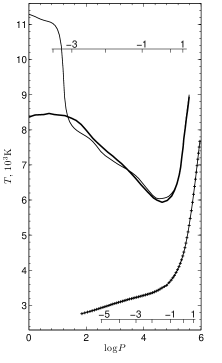
Figure 1: Temperature distribution in a stellar atmosphere with $T_{eff}=4100$ K and $\log g=4.5$ as a function of pressure $P$ (dyn cm^-2). The structure of an atmosphere without external heating is shown in the lower part of the figure: the thin solid line indicates the calculation with the unmodified version of ATLAS9; the crosses represent our calculations. The scale under the curve is the logarithm of the Rosseland optical depth for these models. The structure of the same atmosphere but heated by blackbody radiation with $T_{B}=20\,000$ K is shown in the upper part of the figure: the thick and thin solid lines indicate the calculations by Günther and Wawrzyn (2011) and our calculations, respectively. The scale in the upper part of the figure is the logarithm of the Rosseland optical depth for the models with heating.

Subsequently, we compared the model computed using our version of the ATLAS9 code with the calculations performed by Günther and Wawrzyn (2011) using the PHOENIX code, in which hydrogen and helium are taken into account without assuming LTE. We considered a star with the same parameters as those in the preceding case on which blackbody radiation with $T_{B}=20\,000$ K was incident perpendicular to its surface, with the ratio of the external radiation flux $F_{B}$ to the stellar one being 5.31. For comparison with this model, we set $P_{0}=0$ in our code and replaced the shock radiation spectrum by a blackbody one with the following characteristics:

$$I_{\nu}^{0}(\mu)=F_{B}\delta(\mu+1)\delta(\varphi),\quad J_{\nu}^{0}=\frac{F_{B}}{4\pi}e^{-\tau_{\nu}},\quad H_{\nu}^{0}=-\frac{F_{B}}{4\pi}e^{-\tau_{\nu}},$$

where $\delta(x)$ is the delta function. In our code, we additionally specified the microturbulence $v_{t}=1$ km s^-1 and the parameter describing convection $l/H_{p}=2.$

As we see from Fig. 1, the temperature differences in the region with $\log P>2,$ which is of interest in the problem on heating the atmospheres of CTTS by shock radiation, do not exceed 250 K. The models begin to differ greatly at lower values of $P$ to which a Rosseland mean optical depth $\log\tau_{Ross}<-3.3$ corresponds, i.e., where the LTE approximation is barely justified. Therefore, the model computed with the PHOENIX code must yield more realistic results than the ATLAS9 code. It follows from the aforesaid that our modified ATLAS9 code is quite suitable for solving the formulated problem.

Dependence of the vertical hot-spot structure on shock parameters

As has already been pointed out, when calculating the heating of CTTS atmospheres, we used the opacity tables for a microturbulence of 2 km s^-1 and solar elemental abundances. Everywhere below, unless otherwise specified, we took $\log g=4.0$ and, when describing convection, $l/H_{p}=1.25.$ Our calculations were performed on a mesh of 72 Rosseland optical depths from $\log\tau_{Ross}=-5.1$ to $\log\tau_{Ross}=2$ with a step $\Delta\log\tau=0.1.$ Thus, the models considered below differ from one another by the stellar effective temperatures $T_{eff}$ and shock parameters, i.e., by $N_{0}$ and $V_{0}.$

Let us first consider how sensitive the structure of CTTS atmospheres heated by shock radiation is to the angular dependence $I_{\nu}^{0}(\mu).$ For this purpose, we computed two models describing the heating of a star with $T_{eff}=4000$ K by radiation from a shock with $V_{0}=400$ km s^-1 and $\log N_{0}=12.0.$ They differ from each other in that we used dependence (3) in the first case and (4) in the second case.

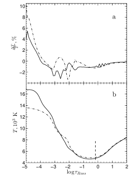
Figure 2: (a) Relative temperature difference between two models in which all parameters are identical but the dependence $I_{\nu}^{0}(\mu)$ is different: it is specified by Eq. (3) in one model and by Eq. (4) in the other model. The solid line is for the pair of models with $V_{0}=400$ km s^-1 and $\lg N_{0}=12.0;$ the dash-dotted line is for $V_{0}=200$ km s^-1 and $\log N_{0}=12.9.$ The Rosseland mean optical depth is along the horizontal axis. (b) The temperature distribution in an atmosphere heated by shock radiation with an isotropic dependence of the incident radiation (4) and $V_{0}=400$ km s^-1 and $\log N_{0}=12.0$ (solid line), $V_{0}=200$ km s^-1 and $\log N_{0}=12.9$ (dash-dotted line). The vertical dashed line marks the position of $\tau_{Ross}=2/3$.

Since here we calculate LTE spectra, the difference in temperature distribution for these models is of chief interest. The solid line in Fig. 2 indicates the relative temperature difference $\Delta T/T$ of the pair of models under consideration as a function of the optical depth $\tau_{Ross}.$ We see that $\Delta T/T\leq 3$ % in the region $\log\tau_{Ross}>-4$. An equally small difference is also obtained when comparing the pair of models with other identical shock parameters and $T_{eff}$ of the star but with different laws $I_{\nu}^{0}(\mu)$ – see, for example, the dash-dotted curve in the same plot that indicates the result of our calculations for $T_{eff}=4000$ K, $V_{0}=200$ km s^-1, $\log N_{0}=12.9.$ Consequently, the uncertainty in choosing the law $I_{\nu}^{0}(\mu)$ in the problem on heating of the atmospheres of CTTS by shock radiation may be considered to be of no fundamental importance, and we will always assume below that the shock radiation intensity is isotropic, i.e., described by law (4).

Let us now examine how the structure of the atmosphere being heated changes with shock parameters. For this purpose, we will fix the star’s effective temperature and consider a pair of models with different parameters $N_{0}$ and $V_{0}$ but with identical accretion energy fluxes $F_{ac}=\int F_{\nu}^{sh}{\rm d}\nu\simeq\rho_{0}V_{0}^{3}/4.$

The dash-dotted and solid lines in the lower panel of Fig. 2 indicate the dependence$T=T(\tau_{Ross})$ for the models with $V_{0}=200$ km s^-1 , $\log N_{0}=12.9$ and $V_{0}=400$ km s^-1, $\log N_{0}=12.0$, respectively. Both models were computed for a star with $T_{eff}$ = 4000 K, have the same $F_{a}c$, but differ by the spectral composition of the shock radiation and the pressure $P_{0}$ at the outer atmospheric boundary.

We see from Fig. 2 that in the region with $\tau_{Ross}\gtrsim 2/3$ (this optical depth is marked by the vertical line in the figure), i.e., where the continuum emission originates, the differences between the models are comparatively small. In other words, for models with the same $F_{ac}$, the intensity and spectrum of the emission continuum should be approximately identical. At the same time, the differences in structure become noticeable in the formation region of emission lines: for a softer shock radiation spectrum, i.e., at $V_{0}=200$ km s^-1 in the case under consideration, the layers with a moderately small optical depth are heated slightly more strongly that they are for a harder spectrum, but, on the other hand, the atmosphere for a soft spectrum at quite $\tau_{Ross}$ is heated to a much lesser extent.

It is quite predictable that the structure of the atmosphere being heated depends mainly on the external radiation power or, more precisely, on the parameter $K=F_{ac}/\sigma T^{4}_{eff}.$ This is illustrated by Fig. 3. It shows how the gas temperature and pressure and the electron density change with optical depth $\tau_{Ross}$ for the models that we will use most frequently below. These models are numbered in the figure in order of increasing K: (1) $V_{0}=200$ km s^-1, $\log N_{0}=11.5$ $(K\simeq 0.09);$ (2) $V_{0}=400$ km s^-1, $\log N_{0}=11.5$ $(K\simeq 0.76);$ (3) $V_{0}=200$ km s^-1, $\log N_{0}=12.5$ $(K\simeq 0.94);$ (4) $V_{0}=400$ km s^-1, $\log N_{0}=12.5$ $(K\simeq 7.6).$ In all cases, $T_{eff}=4000$ K.

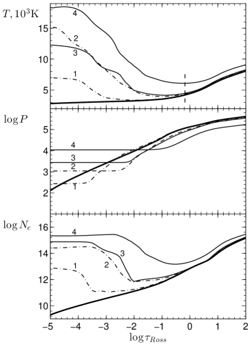
Figure 3: Dependence of the model for the heating of a stellar atmosphere with $T_{eff}$ = 4000 K and $\log g=4.0$ on external radiation properties. $\tau_{Ross}$ is the Rosseland optical depth; the vertical line indicates $\tau_{Ross}=2/3.$ From top to bottom: the temperature ($10^{3}$ K), pressure (dyn cm${}^{-2}),$ and electron density (cm${}^{-3})$ distributions. The thick line indicates the model without heating, 1 – V0 = 200 km s${}^{-1},$ $\log N_{0}=11.5;$ 2 – $V_{0}=400$ km s${}^{-1},$ $\log N_{0}=11.5;$ 3 – $V_{0}=200$ km s${}^{-1},$ $\log N_{0}=12.5;$ 4 – $V_{0}=400$ km s${}^{-1},$ $\log N_{0}=12.5.$

The larger the $K,$ the greater the difference between the structure of the atmosphere being heated and the initial one. At the same time, we see from the figure that the dependence $T=T(\tau_{Ross})$ at $K<1$ in the region with $\tau_{Ross}\gtrsim 2/3,$ i.e., where the continuum originates, is almost the same as that in an unperturbed atmosphere. This means that the depth of photospheric lines can decrease significantly due to the emission continuum only at $K>1.$ Therefore, when interpreting the spectra of noticeably veiled CTTS, Calvet and Gullbring (1998), who disregarded the emission in lines in their calculations, always obtained a large $K.$

Computing the Spectrum

Having determined the structure of the atmosphere being heated, we computed the spectrum of the emergent radiation from it using the SYNTHE code in the ATLAS9 package. In contrast to Calvet and Gullbring (1998), we calculated not the flux $H_{\nu},$ but the intensity of the emergent radiation from the hot spot $I_{\nu}^{spot}(\mu)$ for 17 values of $\mu$ from 1.0 to 0.01.

In our calculations, we took into account both the continuum and all the lines of atoms, ions, and molecules available in the ATLAS9 package. The spectral resolution $R\equiv\lambda/\Delta\lambda$ in our calculations was $\simeq 600\,000.$

Before reaching the observer, the hot-spot radiation passes through the material both downstream and upstream of the shock front. However, it turned out that in the visible range at $V_{0}$ and $N_{0}$ of interest to us, the gas falling to the star hardly distorts the spectrum and intensity of the hot-spot radiation. This is mainly attributable to a very small optical depth of the accreting gas in continuum $\lambda>4000$ Å  (Calvet and Gullbring 1998; Lamzin 1998). As regards the lines, they must be redshifted in the gas moving toward the star, while only a very small number of lines in the visible range have noticeable absorption and/or emission components in the red wing in the optical spectra of CTTS (see, e.g., Petrov et al. 2001). The results of modeling the profiles of such lines are to be presented in the immediate future.

Figure 4 shows how the radiation spectrum of a plane-parallel layer with $T_{eff}=4000$ K (dotted curve) changes as it is heated by shock radiation with $K=0.09,$ 0.76, and 2.6 (solid curves). To be more precise, the dependencies $I_{\lambda}(\lambda)$ are shown in the left and right panels of the figure for the cases where the line of sight makes, respectively, the angles $\alpha=0^{o}$ and $\alpha=60^{o}.$ with the normal to the layer. For clarity, the spectra were normalized to the continuum level $I_{c}^{0}$ of a layer without external heating $(K=0).$

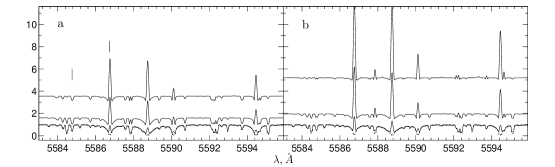
Figure 4: Portion of the spectrum for a plane layer with $T_{eff}=4000$ K (dotted line) and the same layer heated by shock radiation at different K: for a layer with the normal to its surface making the angles $\alpha=0^{o}$ (a) and $\alpha=60^{o}$ (b) with the line of sight. The three curves in each panel correspond to the spectra of the models with the following parameters (from bottom to top): $V_{0}=200$ km s^-1 and $\log N_{0}=11.5$ $(K\simeq 0.09),$ $V_{0}=200$ km s^-1 and $\log N_{0}=12.5$ $(K\simeq 0.76),$ $V_{0}=400$ km s^-1 and $\log N_{0}=12.5$ $(K\simeq 2.6).$ The vertical bars mark the positions of two Fe I lines with $gf$ differing by a factor of 160. The layer radiation intensity $I_{\lambda}$ normalized to the continuum intensity of a layer without heating is along the vertical axis.

Let us first consider the behavior of the spectra for $\alpha=0^{o}.$ We see that the continuum intensity at $K=0.09$ (lower solid curve) remained essentially the same, but the depth of some absorption lines, for example, Fe I $\lambda$ 5586.8 and Ca I $\lambda$ 5588.8, decreased appreciably. The continuum level at $K=0.76$ (middle solid curve) increased approximately by a factor of 1.6, while the depth of absorption lines decreased to an even greater extent and some of them turned into emission ones. This effect is even more pronounced in the spectrum at $K=2.6$ (upper curve). If we now take a look at the right panel of the figure, which corresponds to the case of $\alpha=60^{o},$ then we will see that the picture did not change qualitatively, but the continuum level increases faster with increasing $K,$ while the emission lines appear already at $K=0.09.$

These peculiarities can be understood by taking into account the following facts: (1) in the LTE approximation, the intensity of radiation at a given wavelength is approximately equal to the value of the Planck function in a region with an optical depth $\tau_{\lambda}\simeq 1;$ (2) a temperature inversion arises in an atmosphere heated by shock radiation, with the position of the temperature minimum shifting to increasingly large $\tau_{Ross}$ as $K$ increases (see the upper panel of Fig. 3).

The intensity of the spot radiation in continuum at $K\simeq 0.1$ is almost equal to $I_{c}^{0},$ because the temperature $T_{eff}$ at $\tau_{Ross}\simeq 1$ changed very little compared to what it was in the absence of heating – see curve 1 in the upper panel of Fig. 3. The lines are formed at smaller $\tau_{Ross},$ where the relative rise in temperature is larger. Therefore, their intensity increases to a greater extent than it does in the adjacent continuum, causing the depth of absorption lines to decrease, i.e., their veiling. Depending on how large the absorption coefficient of a line is, it originates in a region with a temperature that is either lower or higher than that in the formation region of the adjacent continuum. The line will appear as an absorption one in the former case and as an emission one in the latter case. There are no emission lines at $K=0.1$ in the portion of the spectrum shown in Fig. 4, but they are present in other portions of the spectrum – for example, the Fe II $\lambda$ 5234.6 line, while the emission line also appear in the chosen portion as $K$ increases. The behavior of the two Fe I lines with $\lambda=5584.8$ and $\lambda=5586.8,$ for which $\log gf$ is -2.32 and -0.12, respectively, can serve as an illustration of the aforesaid.

If we look at the layer not along the normal to its surface but at an angle, then the outermost atmospheric layers, whose temperature at $\mu=0.5$ is higher than that at $\mu=1$, will correspond to $\tau_{\lambda}=1.$ In other words, for the hot spot, just as for the solar chromosphere, the law $I_{\lambda}=I_{\lambda}(\mu)$ corresponds not to limb darkening but to limb brightening; we see from Fig. 4 that the dependence $I(\mu)$ in the case of lines is steeper than that for the continuum. As regards the quantitative differences in continuum level at the same $K$ but different $\mu,$ it should be remembered that the curves $I_{\lambda}(\lambda)$ in the figure are normalized to the continuum level of an unperturbed atmosphere, where $I_{\lambda}(0.5)<I_{\lambda}(1).$

To compare our calculations with observations, we assumed here that on the stellar surface there was only one circular spot within which the shock parameters, i.e., $V_{0}$ and $N_{0},$ were identical. The position of the spot in this case is determined only by the angle between the normal at the spot center and the line of sight. Another characteristic of the spot is $f,$ the ratio of its area to the surface area of the entire star.

The radiation coming to the observer is the sum of the radiations from the spot and the unperturbed stellar surface. The observed flux $F_{\lambda}$ is obtained by integrating the intensity $I_{\lambda}(\mu)$ over the solid angle:

$$F_{\lambda}={R_{*}^{2}\over d^{2}}\,\int{I_{\lambda}(\mu)\,\mu\,\sin\theta\,{\rm d}\phi\,\,{\rm d}\theta},$$

where $\theta$ and $\phi$ are the spherical coordinates of the points on the surface of a star with radius $R_{*}$ at distance $d$ from us, and $\mu=\mu(\theta,\phi)$ is the cosine of the angle $\alpha$ between the local normal to the surface and the line of sight. In our calculations, we used a uniform $100\times 100$ coordinate grid in $\theta$ and $\phi$ for each cell of which we can write

$$I_{\lambda}(\theta,\phi)=\begin{cases}I_{\lambda}^{star},\text{ if $(\theta,\phi)\notin\Pi$ }\\ \\ I_{\lambda}^{spot},\text{ if $(\theta,\phi)\in\Pi$ },\\ \end{cases}$$

where $\Pi$ is the domain of $\theta$ and $\phi$ in which the hot spot is specified.

Comparison of the calculation with observations

The relative contribution of lines and continuum to the veiling

Evidence for the presence of emission lines inside photospheric absorption lines has been found in stars with heavily veiled spectra: RU Lup, S CrA NW, S CrA SE (Gahm et al. 2008), DR Tau (Petrov et al. 2011). For each of these stars, we were able to select a model whose spectrum, as can be seen from Fig. 5, is rather similar to the observed one, at least in that the lines exhibiting an emission feature in the observed spectra also exhibit emission features in the models. The observed spectrum is shown in the upper part of each panel in the figure, and the thin solid line below indicates the model spectrum for a star with a hot spot whose parameters are given in the table. Both spectra were normalized to the continuum level, but, for clarity, they were shifted from $F_{\lambda}/F^{c}_{\lambda}=1$ vertically. In addition, the calculated spectra were broadened by its convolution with a Gaussian with $\sigma=7.5$ km s^-1 in order that their spectral resolution be the same as that of the observed ones.

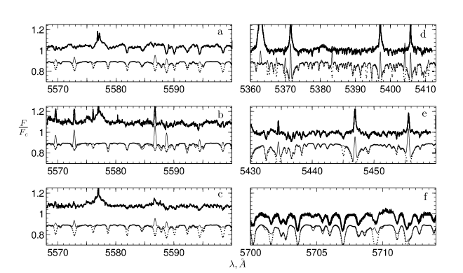
Figure 5: Calculated and observed spectra of heavily veiled CTTS. The thick curve indicates the observed spectrum: (a) RU Lup, (b) S CrA SE, (c) S CrA NW (Gahm et al. 2008), (d) and (e) DR Tau (Petrov et al. 2011), (f) RU Lup (Stempels and Piskunov 2003). The thin solid line indicates the spectra of the models from the table, while the dotted line indicates the spectra of the same models calculated by disregarding the emission in lines. The spectra were normalized to the continuum level but were shifted vertically for the convenience of comparison.

Table 1: Parameters of the models for heavily veiled stars

#	Star	$r$	$f$	$\log N_{0}$, cm-3	$V_{0},$ km s-1	$T_{2/3}$, K	$R_{*}/R_{\odot}$	$\dot{M},$ $M_{\odot}$ yr-1
1	RU Lupa	6	0.12	12.5	400	6100	1.7d	$9\times 10^{-8}$
2	S CrA NWa	8	0.12	12.5	400	6100	1.2e	$5\times 10^{-8}$
3	S CrA SEa	5	0.15	12.5	300	5200	1.5e	$7\times 10^{-8}$
4	DR Taub	2.5	0.10	12.5	300	5200	1.5b	$4\times 10^{-8}$
5	RU Lupc	2.2	0.15	12	400	4800	1.7d	$4\times 10^{-8}$
Note. $T_{2/3}$ is the hot-spot temperature at $\tau_{Ross}=2/3,$ $R_{*}$ is the stellar radius, $N_{0}$ and $V_{0}$ are the pre-shock gas density and velocity, $r$ is the average veiling level in the range of the corresponding spectrum (Fig. 5), $\dot{M}$ is the accretion rate. The spectra and parameters of the stars were taken from the following papers: (a) Gahm et al. (2008); (b) Petrov et al. (2011); (c) Stempels and Piskunov (2003); (d) Stempels and Piskunov (2002); (e) Carmona et al. (2007).

As we see from the figure, the weak emission lines of the atmosphere being heated to a certain extent blend the photospheric absorption lines, while the strongest ones manifest themselves in the spectra as the so-called narrow emission components (see the Introduction). It is important to note that the calculated intensity of the narrow components in metal lines is much lower than the observed intensity of the corresponding emission lines. This is entirely consistent with the conclusion that the emission lines of metals consist mainly of the so-called broad component forming outside the hot spot: Batagla et al. (1996) and Petrov et al. (2001) reached this conclusion by analyzing the profile variability, while Dodin et al. (2012) showed that for RW Aur the magnetic field in the formation region of metal emission lines is much weaker than that in the hot spot.

Below, we will discuss how well the model parameters from the table can describe the corresponding stars, while now we will ascertain to what extent and under what conditions allowance for the emission lines influences the veiling. The first impression can be gained even from Fig. 5, in each panel of which the dotted curve indicates the spectrum of the corresponding model from the table computed using the SYNTHE code but without any allowance for the spectral lines. In other words, this is the spectrum of a star with a hot spot veiled only by the emission continuum.

The value of the following quantities averaged over the spectral range of interest to us is traditionally used as a measure of veiling of the CTTS spectra:

$$r(\lambda)={EW_{0}(\lambda)\over EW(\lambda)}-1.$$

They show the extent to which the equivalent widths of photospheric lines $EW$ in the spectrum of CTTS differ from the equivalent widths $EW_{0}$ of the same lines in the spectrum of a comparison star. Up until now, the comparison star is chosen in such a way that the sum of its spectrum and a constant-intensity ”veiling continuum” in a comparatively narrow wavelength range fits best the spectrum of the star being studied (see, e.g., Petrov et al. 2001). The difference in $r$ for different lines was assumed to be due to observational errors and/or not quite an appropriate choice of the comparison star.

For our models, $r$ were determined by comparing two computed spectra: stars with and without a hot spot. In this case, we took two overlapping spectral lines as one if there were no local maxima inside the blend profile (the lines were indistinguishable); otherwise we considered the lines separately and regarded the point of maximum as the boundary between them. Recall that we compute the models in the LTE approximation, which definitely breaks down at very small $\tau_{Ross},$ i.e., in the formation region of the strongest lines. Therefore, in determining $r$ we used only sufficiently weak lines originating in layers where the LTE hypothesis seems justified. On the other hand, there was no point in taking into account very weak lines $(EW<0.03$ Å ), because they are masked by noise in the observed spectra.

As the external radiation power increases, the degree of veiling of the spectrum for a star with a hot spot grows. Figure 6 gives an idea of the quantitative magnitude of the effect. As an example, it shows the dependence $r(K)$ in the range 5500-6000 Å  for a moderate-size hot spot $(f=6\,\%)$ on the surface of a star with $T_{eff}=4000$ K (Fig. 6a) and $T_{eff}=5000$ K (Fig. 6d). The thick and thin lines correspond to the cases where the spot symmetry axis makes, respectively, the angles $\alpha=0^{o}$ and $\alpha=60^{o}$ with the line of sight.

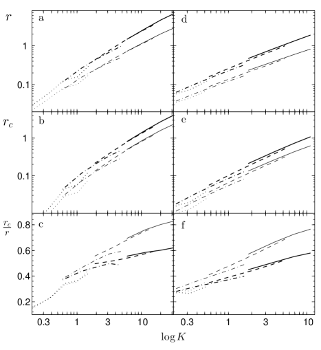
Figure 6: Quantities $r$ (upper row), $r_{c}$ (middle row), and their ratio (lower row) in the range 5500-6000 Å  versus relative shock radiation power in the case of a spot that occupies 6% of the surface of a star with $T_{eff}=4000$ K (left column) and $T_{eff}=5000$ K (right column). Each line corresponds to a series of models with identical $N_{0}$ but different $V_{0}$ from the range 200-400 km ${}^{-1}.$ The solid, dashed, dash-dotted, and dotted lines are for $\log N_{0}=13.0,$ $12.5,$ $12.0,$ and $11.5,$ respectively. The thicker and thinner lines correspond to a spot observed at $\alpha=0^{o}$ and $\alpha=60^{o},$ respectively.

If the equivalent widths changed only through a change in the continuum level, then the veiling could be characterized by the parameter

$$r_{c}(\lambda)={F_{\lambda}\over F^{0}_{\lambda}}-1,$$

where $F_{\lambda}$ and $F^{0}_{\lambda}$ are the continuum fluxes for the accreting and nonaccreting stars, respectively. The ratio $r_{c}/r$ shows what fraction of the ”true” veiling is attributable to the emission continuum alone.

Figures 6b, 6e and 6c, 6d show how $r_{c}$ and $r_{c}/r,$ respectively, change as the shock radiation power increases for the same spots and in the same spectral range. We see that both $r_{c}$ and $r_{c}/r$ increase with $K.$ This means that the contribution of lines to the spectrum veiling is largest when r is comparatively small (in our case, $r_{c}/r<0.5$ at $r<0.3-0.4).$ However, we have already seen this for the radiation of a plane layer as an example (see the previous section and Fig. 4).

In the opinion of Petrov et al. (2011), if the contribution of lines to the veiling is disregarded, then the accretion rate will be overestimated most for stars with large $r$. It follows from Fig. 6 that, in general, this is not true. Suppose, for example, that in the case of a star with $T_{eff}=4000$ K and a spot with $f=0.06,$ $r=0.1$ was obtained from observations at $\alpha=0^{o},$ which, neglecting the contribution of lines, is mistaken for $r_{c}.$ Using the figure, we find that as a result of the misinterpretation, we will obtain $K$ that is twice the correct one. However, if the observed degree of veiling for the same star is $r=3,$ then the error in $K$ will be not larger but, on the contrary, smaller approximately by a factor of 1.5. Assuming, for simplicity, that $V_{0}$ was correctly determined from observations, we will obtain the same errors for the accretion rate as well.

It may appear that the lines for stars with a high veiling level should be considered as an insignificant correction. However, this is not the case, and we will now discuss a number of qualitatively new effects that arise when the emission in lines is taken into account.

Figure 7 shows how $r$ and $r_{c}$ change in different regions of the spectrum for model no. 5 from the table. We chose this model for comparison with the spectrum of RU Lup taken from Stempels and Piskunov (2003): a small region of this spectrum is presented in Fig. 5f. In accordance with the aforesaid, all points in the figure lie above the line $r_{c}=r_{c}(\lambda);$ in this case, $r$ averaged over small regions of the spectrum are considerably larger than $r_{c},$ i.e., there is veiling mainly by lines, not by the emission continuum, especially in the short-wavelength part of the spectrum.

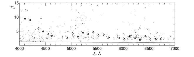
Figure 7: Wavelength dependence of the veiling. For model no. 5 from the table, the dots indicate the values of $r$ obtained from individual lines, while the solid line indicates the dependence $r_{c}(\lambda).$ The diamonds represent the average veiling in narrow regions of the spectrum for RU Lup determined by Stempels and Piskunov (2003).

As we see from the figure, the values of $r$ can differ by several times even for closely spaced lines. The quantity $r$ has a particularly large scatter in the wavelength range 5000-5500 Å. As a result, its mean value in this range increases, with such a peculiarity taking place in all of our computed models. Thus, the local maximum in the dependence $r=r(\lambda)$ near $\lambda\approx 5300$ Å found by Stempels and Piskunov (2003) for RU Lup and by Hartigan et al. (1989) for BP Tau cannot be considered as evidence for a nonmonotonic energy distribution of the veiling continuum in the visible spectral range.

Unless we take into account the fact that the veiling by lines changes the depth of photospheric lines to a very different degree even within a narrow spectral range, the universally accepted method of determining the effective temperatures of CTTS (Hartigan et al. 1989) by comparing $EW$ of absorption lines in the spectrum of the program and comparison stars must yield erroneous results. Using this technique, we processed our computed model spectra for a star with a hot spot at two spot positions relative to the observer: $\alpha=0^{o}$ and $\alpha=60^{o}.$ The error of the method by Hartigan et al. (1989) can be estimated by comparing $T_{eff}$ obtained in this case with the value taken when computing the model. We used our computed grid of spectra for stars without a spot with $\log g=4.0$ and $T_{eff}$ from 3500 to 5750 K with a step of 250 K as comparison spectra.

The results turned out to be ambiguous: the difference $\Delta T_{eff}$ between the calculated and actual values of $T_{eff}$ most commonly did not exceed 250 K, i.e., no more than one spectral subtype, but, in some cases, the differences were considerably larger. For example, for model no. 5 from the table at $\alpha=0^{o},$ we found $\Delta T_{eff}=+1750$ K over the spectral region 4500-5000 Å, $\Delta T_{eff}=-250$ K in the range 5000-5500 Å, and $\Delta T_{eff}=0$ K over regions 500 Å in width at $\lambda>5500.$ In models with a moderately large degree of veiling of the stellar spectrum, the error in $T_{eff},$ as would be expected, is small, but for models with an appreciable veiling, $\Delta T_{eff}$ changes from model to model without any apparent regularity. This is probably because as the degree of veiling increases, some of the photospheric lines either become very weak or turn into emission ones and we cease to take them into account when calculating $r.$ In other words, in different models, $r$ within the same spectral range, in general, is calculated from different set of lines. Therefore, it is reasonable to assume that for all CTTS with an appreciably veiled spectrum (see, e.g., Gullbring et al. 1998), $T_{eff}$ and the spectral type were determined with an error whose value is difficult to predict, especially since the observed spectra of CTTS, in contrast to the model ones, are distorted by noise.

The error in determining $T_{eff}$ for CTTS with an appreciably veiled spectrum leads to an error in estimating the interstellar extinction toward these stars. Therefore, note that $A_{V}$ determined from optical CTTS spectra systematically exceed $A_{V}$ found by analyzing ultraviolet spectra (see Lamzin (2006) and references therein). Lamzin (2006) provided arguments that some systematic error built in the technique of determining $A_{V}$ from optical spectra is responsible for the effect. It is reasonable to assume that this error results from the neglect of the contribution of lines to the veiling.

As the star rotates, the radial velocity of the hot-spot lines changes, causing the centroid of the veiled photospheric lines to be shifted periodically. This is perceived as variability of their radial velocity $V_{r}$ (Zaitseva et al. 1990; Petrov et al. 2001, 2011). However, when this effect is interpreted quantitatively, it should be remembered that all photospheric lines are veiled to a different degree and, hence, the $V_{r}$ variability amplitude will depend on the set of lines used. This is illustrated by Fig. 8, in which $V_{r}$ of photospheric lines from the range 5500-6000Å normalized to the star’s equatorial rotation velocity $V_{eq}$ is plotted against their degree of veiling $r.$

The upper panel in the figure presents the results of our calculations for model no. 3 from the table in the case where a large spot $(f=0.15)$ is located at the equator and is observed at $\alpha=60^{o},$ while the lower panel presents the results for the same parameters of a spot but with a smaller size $(f=0.01).$ The dependence $V_{r}(r)$ is well fitted by a straight line whose equation can be easily derived analytically. This requires finding the centroid of two Gaussians that approximately reproduce the absorption and emission parts of the line, which gives $V_{r}=(r-r_{c})V_{s}\,\xi,$ where $r$ is the total veiling, $r_{c}$ is the continuum veiling, $V_{s}=V_{eq}\sin{i}\sin{\theta}\sin{\phi}$ is the line-of-sight projection of the velocity of the surface element with a spot, $\xi$ is a factor approximately equal to one for a compact accretion zone $(f\lesssim 0.01)$ and 0.3 for $f=0.15$.

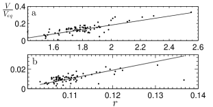
Figure 8: Radial velocity of photospheric lines versus veiling in them: (a) for model no. 3 from the table $(f=0.15)$ at $\alpha=60^{o},$ the dots represent individual lines, the straight line is an analytical fit: $V/V_{eq}=0.3\times(r-1.3)\sin\alpha;$ (b) the same for a spot with $f=0.01$, a fit: $V/V_{eq}=1.0\times(r-0.1)\sin\alpha.$

The presence of emission components inside absorption lines also affects the estimate of the star’s projected equatorial rotation velocity $v\sin{i}.$ The full width at half maximum of the line $(FWHM)$ increases when the emission component is at the line center (the hot spot passes through the central meridian), but the photospheric line becomes narrower when the emission component is in one of the wings. The variability of $v\sin{i}$ in the spectrum of RW Aur (Petrov et al. 2001) is probably attributable precisely to this effect.

Just as for the radial velocities, the result of measuring $v\sin{i}$ depends on which photospheric lines will be chosen. Figure 9 shows how the ratio of $FWHM$ for a line in an accreting star to $FWHM$ for the same line in a star without a spot changes with $r.$ The results are presented for model no. 3 from the table at $\alpha=0^{o}$ and $\alpha=60^{o},$ while the equatorial rotation velocity was taken to be 12 km s${}^{-1}.$ For simplicity, we assumed the spot center to lie at the stellar equator and the inclination of the rotation axis to the line of sight to be $i=90^{o}$. The lines were chosen from the range 5500-6000 Å in such a way that the emission part did not distort the profile too strongly and it could be taken as an ordinary photospheric line in the observed spectrum.

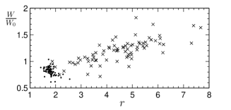
Figure 9: Line broadening versus veiling for model no. 3 from the table. $W/W_{0}$ is the ratio of $FWHM$ for a line in the spectrum of an accreting star to its value in the spectrum of a star without a spot, $r$ is the veiling. The equatorial rotation velocity is $V_{eq}=12$ km s${}^{-1}.$ The crosses and dots indicate a hot spot observed at $\alpha=0^{o}$ and $\alpha=60^{o},$ respectively.

We see from the figure that depending on the choice of lines from which $v\sin{i}$ is determined, the values obtained for this quantity can differ several fold. This suggests that all of the published values of $v\sin{i}$ for CTTS with a noticeably veiled spectrum have a systematic error whose value is difficult to estimate. Precisely this is probably responsible for the problems that arise in attempting to reconcile the rotation period of the star, its radius, and $i$ and $v\sin{i}$ between themselves for DI Cep and RW Aur (Gameiro et al. 2006; Dodin et al. 2012).

Reliability of determining the hot-spot parameters

Here, we consider a comparatively simple model – a circular homogeneous spot. However, the calculations by Romanova et al. (2004) show that even in the simplest case of a dipole stellar magnetic field, the cross section of the accretion stream has a complex shape, while the distributions of $N_{0}$ and $V_{0}$ in this cross section are very nonuniform. Nevertheless, even our simple model allows us to see how large the errors in the parameters characterizing the accretion onto CTTS ($\dot{M},$ $f,$ etc.) are if we use inadequate quality spectroscopic observations and disregard the emission in lines when interpreting the veiling.

Let us first show that several models that reproduce the observed spectra with approximately the same accuracy can be selected within the approximation used. One of the main factors leading to an ambiguity in determining the accretion parameters is the spot position on the stellar surface at the time of observation. Let us illustrate this assertion using the portion of the spectrum for RU Lup displayed in Fig. 5a as an example. The observed spectrum of the star taken from Gahm et al. (2008) is compared in this panel with the model corresponding to a spot with $\alpha=0$ and $f=0.12.$ The remaining model parameters are given in the first row of the table.

Figure 10a shows the relative difference between the spectra for this model and the model in which $f=0.245$ and $\alpha=60^{o},$ while the remaining parameters are the same. In these models, the accretion rates $\dot{M}$ differ approximately by a factor of 2, but we see from the figure that their spectra coincide to within 1 % in the presented portion. To choose between the two models, observational data with a resolution $R>40\,000$ and a signal-to-noise ratio $(S/N)$ of at least 200 should be available. This shows that the published accretion rates estimated from only one spectrum and, what is more, of comparatively low quality cannot be considered reliable even if we forget that the contribution of lines to the veiling was disregarded in this case.

Note that the position of the emission peak inside an absorption line, which must change periodically due to the star’s rotation about its axis, can serve as additional information that allows the angle $\alpha$ to be determined. Such information can be extracted only if several spectra taken at different positions of the spot relative to the observer are available.

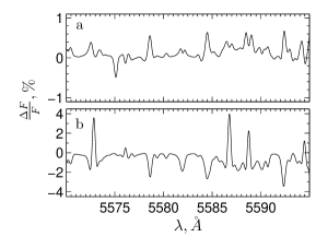
Figure 10: Difference between the spectra $F_{\lambda}(\lambda)$ for two models with different parameters. (a) For models in which only $f$ and $\alpha$ differ. These parameters are, respectively, 0.120 and $0^{o}$ for the first model and 0.245 and $60^{o}$ for the second model. The spectra were broadened by their convolution with a Gaussian to correspond to the observed spectrum of RU Lup shown in Fig. 5. (b) For models in which only $V_{0}$ and $\lg N_{0}$ differ at the same $K$. These parameters are $400$ km s^-1 and $12.0$ for the first model and $200$ km s^-1 and $12.9$ for the second model. The spectra were broadened by their convolution with a Gaussian at $\sigma=7.5$ km s${}^{-1}.$

Since the structure of the atmosphere being heated is determined mainly by the incident radiation power, the spectra of models with identical $K$ are very similar. This is illustrated by Fig. 10b. It shows the relative difference between the spectra of two models with identical $K$ but different $V_{0}$ and $\log N_{0},$ which are, respectively, $400$ km s${}^{-1},$ $12.0$ and $200$ km s${}^{-1},$ $12.9.$ The accretion rates in these models differ by a factor of 4, but the relative difference between $F_{\lambda}$ in the spectral range under consideration is $<4$ %. Such a difference can be seen only at a spectral resolution $R>30\,000$ and $S/N>50.$

It also follows from our calculations that the spectra of models with the same $\dot{M}$ but different $f$ and $N_{0}$ at a given $V_{0}$ can be distinguished under approximately the same requirements for the quality of spectroscopic observations as those when comparing the models with the same $K.$

For our comparison with the spectra of CTTS in Fig. 5, we chose models whose spectra were qualitatively similar to the observed ones: within the model of a homogeneous circular spot, there is no point in achieving the best quantitative agreement between the calculated and observed spectra. In all cases, we took $T_{eff}=4000$ K and $\log g=4.0$ Since the models with greatly differing parameters can have very similar spectra, the quantities given in the table cannot be regarded as the true characteristic of the corresponding CTTS. Using the published radii of these stars, we estimated the accretion rate for them. Although these estimates are exclusively illustrative, it is worth noting that compared to $\dot{M}$ obtained without allowance for the veiling by lines (Gullbring et al. 2000; Lamzin et al. 1996), our values are lower by a factor of 3-10.

Thus, even to determine the parameters of a circular homogeneous spot $(N_{0},$ $V_{0},$ $f,$ $\dot{M})$ and its position on the stellar surface, several high-quality spectra that must be taken during the star’s complete turn about its axis should be available. The effective temperature of the star, which is not known in advance for CTTS, should also be determined simultaneously. In fact, however, an even more complex problem should be solved: to determine the shape of the accretion spot and the distribution of $N_{0}$ and $V_{0}$ inside it. Basically, we are talking about the Doppler mapping of CTTS that should be based on model atmospheres heated by shock radiation. Numerous photospheric lines of metals whose depth changes differently due to the emission components even within a narrow spectral range should be used in such a mapping.

Our calculations are the first fundamentally important step in solving this problem: we not only have taken into account the hot-spot emission in lines for the first time but also, in contrast to Calvet and Gullbring (1998), calculated not the flux but the intensity of the spot radiation in different directions, without which no Doppler mapping is possible in principle. The next step is to take into account the departures from LTE when calculating the intensity of the lines that originate in a region with $\log\tau_{Ross}>-3,$ where there is no need to take into account the non-LTE effects when calculating the atmospheric structure, i.e., the dependencies of the ionization fraction and $T,$ $N_{e}$ on $\tau_{Ross}.$

Allowance for the departures from LTE for these lines may turn out to be important in interpreting the spectra: in particular, P.P. Petrov (private communication) found that the photospheric Ca I lines in the spectrum of RW Aur A, in contrast to the lines of other metals, are veiled only by the continuum. Our LTE calculations do not allow this effect to be explained. However, it can be related to a calcium deficiency in the accreting gas. Indeed, as can be seen, for example, from Fig. 5 in the review by Spitzer and Jenkins (1975), the calcium deficiency can be fairly large in the interstellar medium.

Conclusions

Petrov et al. (2001), Gahm et al. (2008), and Petrov et al. (2011) provided arguments that the decrease in the depth of photospheric lines in the spectra of CTTS was due to not only the presence of an emission continuum but also a partial filling of absorption lines with emission ones. As has been shown here for the first time, this effect stems from the fact that a stellar atmosphere heated by shock radiation at the accretion column base (the so-called hot spot) radiates in both continuum and lines, because the temperature above the spot photosphere increases outward. It follows from our calculations that the strongest of these lines manifest themselves in the spectra of CTTS as the so-called narrow emission components, while the weaker ones to a certain extent blend the photospheric lines.

The models of stellar atmospheres heated by external radiation were also computed before us, but the results of these computations could not be used to determine the radiation spectrum of the hot spots on CTTS for the following reasons. In the works devoted to the reflection effect in binary systems, the external radiation spectrum differs greatly from the radiation spectrum of the accretion shock, while the external radiation source is far from the stellar surface. Therefore, this radiation is appreciably diluted and the pressure at the outer boundary of the irradiated atmosphere is zero. Calvet and Gullbring (1998) calculated a series of model atmospheres heated by accretion shock radiation with a nonzero pressure at the outer boundary. However, they disregarded the emission in lines when calculating the spectrum of these atmospheres, because they assumed the veiling in CTTS to be attributable to the continuum alone.

Our calculations of the structure and spectrum of the hot spot were performed using the ATLAS9 code (Kurucz 1970) that we modified in the LTE approximation for a plane-parallel layer with solar elemental abundances. Test calculations showed that the code worked properly. The main parameters of the problem turned out to be the velocity $V_{0}$ and density $N_{0}$ of the pre-shock accreting gas and the stellar temperature $T_{eff}.$ The spot spectrum depends mainly on the ratio $K$ of the external radiation power to the radiation power of an unperturbed atmosphere; the spot emission occurs mainly in lines at small $K,$ while a noticeable emission in continuum appears at larger $K.$ At identical $K$ but different $V_{0}$ and $N_{0},$ the differences between the spot spectra are small. However, it should be remembered that the shape of the spectra in the LTE approximation is determined primarily by the dependence $T=T(\tau_{Ross}).$ Therefore, takin into account the departures from LTE can change significantly this conclusion.

Assuming that there is one circular spot within which $V_{0}$ and $N_{0}$ are the same on the surface of a star with $T_{eff}$ from 3750 to 5000 K, we calculated how the resulting spectra of the star$+$spot should appear at different relative sizes of the spot $f$ and its positions relative to the observer characterized by the angle $\alpha$ between the line of sight and the spot symmetry axis. For each of the stars in which the veiling by lines was detected (Gahm et al. 2008; Petrov et al. 2011), we were able to select a model with a spectrum similar to the observed one, at least in that the lines exhibiting an emission feature in the observed spectra also exhibit emission features in the models.

Petrov et al. (2011) pointed out that the accretion rate for CTTS with a heavily veiled spectrum could be overestimated by neglecting the contribution of emission lines to the veiling. Our calculations show that the accretion rate can be overestimated by several times, even for stars with a comparatively weakly veiled spectrum. It turned out that as a result of the veiling by lines, models with distinctly different parameters could have very similar spectra. Therefore, even in the case of a circular homogeneous spot, to determine $N_{0},$ $V_{0},$ $f$, and the spot position on the stellar surface, it is necessary to have several high-quality spectra that should be taken during the star’s complete turn around its axis. Concurrently, the effective temperature of the star should also be determined, whose errors without allowance for the veiling by lines can be rather large.

The spot motion relative to the observer as the star rotates around its axis causes the positions of emission components inside absorption lines to be shifted. This is perceived as variability of the star’s radial velocity. Concurrently, the width of photospheric lines also changes, which appears as variability of $v\sin i.$ It is important to emphasize that the magnitude of the effect depends on precisely which photospheric lines will be chosen for measurements, because the degree of line veiling $r$ can differ by several times even within a comparatively narrow spectral range.

It follows from our calculations that the scatter of $r$ in the visible range is particularly large in the wavelength range 5000-5500 Å, as a result of which its mean value increases in this range. So far the contribution of lines to the veiling has been disregarded; the presence of a local maximum in the dependence $r=r(\lambda)$ near $\lambda\approx 5300$ Å was interpreted as a nonmonotonic spectral energy distribution of the emission continuum whose cause was unclear.

Without allowance for the emission lines, $r$ was a useful characteristic of the relative hot-spot radiation power. However, if the lines are taken into account, then the meaning of $r$ turns out to be by no means obvious. This means that when the spectra of CTTS are described, it makes sense to specify the degree of veiling only by additionally specifying the set of photospheric lines from which $r$ was determined.

In reality, the hot spot is definitely noncircular in shape and the distribution of $N_{0}$ and $V_{0}$ in the cross section of the accretion stream is nonuniform. To reconstruct the actual picture of accretion onto CTTS, these stars should be Doppler mapped based on model atmospheres heated by shock radiation. Numerous photospheric lines of metals whose depths change differently due to the emission components should be used in mapping.

Our calculations are the first step in solving this problem: we not only have taken into account the hot-spot emission in lines for the first time but also, in contrast to Calvet and Gullbring (1998), have calculated not the flux but the intensity of the spot radiation in different directions, without which no Doppler mapping is possible in principle. In the immediate future, we are planning to clarify the role of departures from LTE for the lines that veil the photospheric lines, but not so strongly as to turn them from absorption lines into emission ones.

As regards the helium and metal lines that are in emission in the spectra of CTTS, as our calculations confirm, they consist mainly of the so-called broad component forming outside the hot spot. Subtracting the narrow components associated with the spot from the observed emission line profiles, we hope to obtain information about the profiles of the broad components that will make it possible to clarify the velocity field and physical conditions in their formation region.

ACKNOWLEDGMENTS. We wish to thank L.I. Mashonkina and P.P. Petrov for useful discussions. This work, just as the previous one (Dodin et al. 2012), was supported by the Program for Support of Leading Scientific Schools (NSh-5440.2012.2).

Appendix. Calculating the structure of the pre-shock zone

Lamzin (1998) calculated the shock radiation in the range of wavelengths shorter than $\simeq 2000$ Å, where the radiation intensity from the photospheres of CTTS is low. In the optical range that we consider here, apart from the hot spot, only the pre-shock zone contributes appreciably to the radiation. However, the fact that the pre-shock region reemits half of the incoming short-wavelength radiation of the shock (after the corresponding reprocessing) toward the star is more important to us in this paper. To take this effect into account, we did not modified Lamzin’s code but used the CLOUDY code (Ferland et al. 1998), which was also applied by Calvet and Gullbring (1998) in their calculations.

The CLOUDY code is designed to compute the thermal structure and radiation spectrum of a gas layer on which radiation with a given spectrum is incident from the outside. We used the version of the code for a plane-parallel layer with solar elemental abundances by assuming the external radiation to be the sum of the radiations from the post-shock zone and the hot spot. For simplicity, we assumed that the spot radiated as a black body with an effective temperature $T_{sp}$ defined by the relation

$$\sigma T_{sp}^{4}=\sigma T_{eff}^{4}+{\rho_{0}V_{0}^{3}\over 4}.$$

We took the radiation spectrum of the post-shock zone from Lamzin (1998) for the same values of $V_{0}$ and $N_{0}$ that were used to calculate the hot-spot structure.

The radiation intensity of the post-shock zone was assumed to be the same in all directions. For the intensity of the radiation entering the pre-shock zone, we can then write

$$I_{\nu}=\frac{F_{ac}}{\pi}+B_{\nu}\left(T_{sp}\right).$$

Note that within the isotropic approximation we slightly underestimate the radiation density in the layers adjacent to the shock front while simultaneously overestimating it in more distant layers.

Not the intensity of the external radiation $I_{\nu}$ but its value averaged over the solid angle $4\,\pi$ serves as an input parameter of the CLOUDY code:

$$4\pi J_{\nu}=\int_{4\pi}{I_{\nu}}\,{\rm d}\Omega=2\pi\int\limits_{0}^{1}{\left[\frac{F_{ac}}{\pi}+B_{\nu}\left(T_{sp}\right)\right]}{\rm}{\rm d}\mu=2F_{ac}+2\pi B_{\nu}\left(T_{sp}\right).$$

We took the distance from the shock front to the point at which the gas temperature drops from its maximum value to 6000 K as the layer thickness $H.$ At an expected diameter of the accretion-column cross section $\gtrsim 3\times 10^{10}$ cm (a filling factor $f\gtrsim 0.03$), the layer cannot be considered as a plane-parallel one at a thickness $H\gtrsim 10^{10}$ cm. We limited the thickness of the layer by this value even if the temperature at its outer boundary exceeded 6000 K in this case. Depending on the model, the layer has a thickness $H=5{\times}10^{9}-10^{10}$ cm.

In the CLOUDY code, it is assumed that the irradiated gas layer is stationary, while the pre-shock gas falls to the star with a velocity $V_{0}\sim 300$ km s${}^{-1}.$ Since the thermal and ionization equilibrium is established in a finite time, the temperature distributions in the stationary and moving gases must differ (for more detail, see Lamzin 1998). However, our checking showed that these differences had virtually no effect on the final result – the thermal structure of the hot spot.

To calculate the heating of the stellar atmosphere, we should determine the part of the radiation from the pre-shock zone that is directed to the star. Assuming that this radiation is isotropic, we have the following relation between its intensity $I^{pre}_{\nu}(\mu)$ and the quantity $4\pi J_{\nu}$ calculated by the CLOUDY code:

$$I^{pre}_{\nu}(\mu)={4\pi J_{\nu}\over 2\pi}.$$

The hot-spot radiation passes through the pre-shock region on its way to the observer. The resulting spectrum is the sum of the intrinsic radiation from the region and the spot radiation partially absorbed in it:

$$I_{\nu}(\mu)=I_{\nu}^{spot}(\mu)\,e^{-\frac{\tau_{\nu}}{\mu}}+\int\limits_{0}^{\tau_{\nu}}{S_{\nu}(t)\,e^{\frac{t-\tau_{\nu}}{\mu}}}\,{\rm d}t,$$

where $I_{\nu}^{spot}(\mu)$ is the radiation intensity emergent from the hot spot, $\tau_{\nu}$ is the optical depth of the pre-shock zone at $\mu=1,$ and $S_{\nu}(\tau_{\nu})$ is the source function in the pre-shock zone computed with the CLOUDY code only for the continuum.

At small $\mu,$ the plane-parallel approximation ceases to hold due to the finite cross section of the accretion column. The value of $\mu_{||}$ at which about half of the spot is observed through the side wall can be estimated from the formula

$$\mu_{||}=\left[1+\frac{2f\left(1-2f\right)}{\left(H/R_{*}\right)^{2}}\right]^{-0.5},$$

where $H/R_{*}$ is the ratio of the thickness of the pre-shock zone to the CTTS radius, whose typical value is $\sim 10^{11}$ cm. In our models, the plane-parallel approximation holds for $\mu\gtrsim 0.5$ at $f\sim 0.03.$

References

- [1] C. Bertout, Ann. Rev. Astron. Astrophys. 27, 351 (1989)
- [2] [0.3cm] N. Calvet and E. Gullbring, Astrophys. J. 509, 802 (1998).
- [3] [0.3cm] A. Carmona, M. E. van den Ancker, and Th. Henning, Astron. Astrophys. 464, 687 (2007).
- [4] [0.3cm] F. Castelli and R. L. Kurucz, astro-ph/0405087 (2004).
- [5] [0.3cm] A. V. Dodin, S. A. Lamzin, and G. A. Chuntonov, Astron. Lett. 38, 167 (2012).
- [6] [0.3cm] G. J. Ferland, K. T. Korista, D. A. Verner, et al., Publ. Astron. Soc. Pacif. 110, 761 (1998).
- [7] [0.3cm] G. F. Gahm, F. M. Walter, H. C. Stempels, et al., Astron. Astrophys. 482, L35 (2008).
- [8] [0.3cm] J. F. Gameiro, D. F. M. Folha, and P. P. Petrov, Astron. Astrophys. 445, 323 (2006).
- [9] [0.3cm] E. Gullbring, L. Hartmann, C. Briceño, and N. Calvet, Astrophys. J. 492, 323 (1998).
- [10] [0.3cm] E. Gullbring, N. Calvet, J. Muzerolle, and L. Hartmann, Astrophys. J. 544, 927 (2000).
- [11] [0.3cm] H. M. Günther and A. C. Wawrzyn, Astron. Astrophys. 526, 117 (2011).
- [12] [0.3cm] P. Hartigan, L. Hartmann, S. Kenyon, et al., Astron. Astrophys. Suppl. Ser. 70, 899 (1989).
- [13] [0.3cm] P. Hartigan, S. Edwards, L. Ghandour, Astron. J. 452, 736 (1995).
- [14] [0.3cm] A. H. Joy, Astrophys. J. 110, 424 (1949).
- [15] [0.3cm] A. Königl, Astrophys. J. 370, L39 (1991).
- [16] [0.3cm] R. Kurucz, SAO Sp. Rep. 309 (1970).
- [17] [0.3cm] R. Kurucz, ATLAS9 Stellar Atmosphere Programs and 2 km/s Grid, Kurucz CD-ROMNo. 13 (Smithsonian Astrophys. Observ., Cambridge,MA, 1993).
- [18] [0.3cm] S. A. Lamzin, Astron. Astrophys. 295, 20 (1995).
- [19] [0.3cm] S. A. Lamzin, G. S. Bisnovatyi-Kogan, L. Errico, et al., Astron. Astrophys. 306, 877 (1996).
- [20] [0.3cm] S. A. Lamzin, Astron. Rep. 42, 322 (1998).
- [21] [0.3cm] S. A. Lamzin, Astron. Lett. 32, 176 (2006).
- [22] [0.3cm] P. P. Petrov, G. F. Gahm, J. F. Gameiro, et al. Astron. Astrophys. 369, 993 (2001).
- [23] [0.3cm] P. P. Petrov, G. F. Gahm, H. C. Stempels, et al., Astron. Astrophys. 535, 6 (2011).
- [24] [0.3cm] M. M. Romanova, G. V. Ustyugova, A. V. Koldoba, and R. V. E. Lovelace, Astrophys. J. 610, 920 (2004).
- [25] [0.3cm] N. A. Sakhibullin, Modeling Methods in Astrophysics (FAN, Kazan, 1997) [in Russian].
- [26] [0.3cm] N. A. Sakhibullin and V. V. Shimanskii, Astron. Rep. 40, 62 (1996).
- [27] [0.3cm] L. Sbordone, P. Bonifacio, F. Castelli, and R. L. Kurucz, Mem. Soc. Astron. It. Suppl. 5, 93 (2004).
- [28] [0.3cm] L. Spitzer, Jr. and E. B. Jenkins, Ann. Rev. Astron. Astrophys. 13, 133 (1975).
- [29] [0.3cm] H. C. Stempels and N. Piskunov, Astron. Astrophys. 391, 595 (2002).
- [30] [0.3cm] H. C. Stempels and N. Piskunov, Astron. Astrophys. 408, 693 (2003).
- [31] [0.3cm] J. A. Valenti, G. Basri, and C. M. Johns, Astron. J. 106, 2024 (1993).
- [32] [0.3cm] G. V. Zaitseva, A. G. Shcherbakov, and N. A. Stepanova, Astron. Lett. 16, 350 (1990).
- [33] [0.3cm] Ya. B. Zel’dovich and Yu. P. Raizer, Physics of Shock Waves and High-Temperature Hydrodynamic Phenomena, Vols. 1 and 2 (2nd ed., Nauka, Moscow, 1966; Academic Press, New York, 1966, 1967).
- [34]