Contraction options and optimal multiple-stopping
in spectrally negative Lévy models
Abstract.
This paper studies the optimal multiple-stopping problem arising in the context of the timing option to withdraw from a project in stages. The profits are driven by a general spectrally negative Lévy process. This allows the model to incorporate sudden declines of the project values, generalizing greatly the classical geometric Brownian motion model. We solve the one-stage case as well as the extension to the multiple-stage case. The optimal stopping times are of threshold-type and the value function admits an expression in terms of the scale function. A series of numerical experiments are conducted to verify the optimality and to evaluate the efficiency of the algorithm.
Key words:
Optimal multiple-stopping; Spectrally negative Lévy processes; Real options
Mathematics Subject Classification (2010): Primary 60G40, Secondary 60J75
1. Introduction
Consider a firm facing a decision of when to abandon or contract a project so as to maximize the total expected future cash flows. This problem is often referred to as the abandonment option or the contraction option. A typical formulation reduces to a standard optimal stopping problem, where the uncertainty of the future cash flow is driven by a stochastic process and the objective is to find a stopping time that maximizes the total expected cash flows realized until then. A more realistic extension is its multiple-stage version where the firm can withdraw from a project in stages.
In a standard formulation, given a discount rate and for a standard Brownian motion , and , one wants to obtain a stopping time of that maximizes the expectation
| (1.1) |
The profit collected continuously is modeled as the geometric Brownian motion less the constant operating expense . The value corresponds to the lump-sum benefits attained (or the costs incurred) at the time of abandonment. Here a technical assumption is commonly imposed so that the expectation is finite and the problem is non-trivial. The problem is rather simple mathematically; it reduces to the well-known perpetual American option (or the McKean optimal stopping problem). An explicit solution can be attained even when is generalized to a Lévy process (see, e.g., Mordecki [29]).
In this paper, we generalize the classical model by extending from Brownian motion to a general Lévy process with negative jumps (spectrally negative Lévy process), and consider the optimal stopping problem of the form:
| (1.2) |
We obtain the optimal stopping time as well as the value function for the case is increasing and admits the form for some positive constants , and . We also show the optimality among all stopping times of threshold type (see (2.4) below) when is relaxed to be a general decreasing and concave function. The decreasing property of reflects the fact that the cost of abandoning a project is higher when the project is large.
We further extend it to the multiple-stage case where one wants to obtain a set of stopping times such that a.s. and achieve
| (1.3) |
when and (with ), for each , satisfy the same assumptions as in the one-stage case. The multiple-stopping problem arises frequently in real options (see e.g. [15]) and is well-studied particularly for the case is driven by Brownian motion. In mathematical finance, similar problems are dealt in the valuation of swing options [11, 12] with refraction times between any consecutive stoppings.
Although the use of Brownian motion is fairly common in real options, empirical evidence suggests that the real world is not Gaussian, but with significant skewness and kurtosis (see, e.g., [9, 14, 35]). Dixit and Pindyck [15] considered the case with jumps of a fixed size with Poisson arrivals. Boyarchenko and Levendorskiĭ [10] considered the EPV approach for a general Lévy process satisfying the (ACP)-condition (with a focus on exponential-type jumps for illustration); they solved a related multiple-stage problem with being constant. The Lévy model is in general less tractable than the continuous diffusion counterpart, especially when the lump-sum reward function is not a constant. When jumps are involved, the process can potentially jump over a threshold level, requiring one to compute the overshoot distributions that depend significantly on the form of the Lévy measure. Technical details are further required when it has jumps of infinite activity or infinite variation. For related literature, we refer the reader to, among others, [1, 4, 18, 25, 28] for optimal stopping problems and [6, 7, 16, 21] for optimal stopping games of spectrally negative Lévy processes. For a general reference on optimal stopping problems, see, e.g., [31].
In this paper, we take advantage of the recent advances in the theory of the spectrally negative Lévy process (see, e.g., [8, 24]). In particular, we use the results by Egami and Yamazaki [17], where we obtained and showed the equivalence of the continuous/smooth fit condition and the first-order condition in a general optimal stopping problem. Unlike the two-sided jump case, the identification of the candidate optimal stopping time can be conducted efficiently without intricate computation. The resulting value function can be written in terms of the scale function, which also can be computed efficiently by using, e.g., [19, 33]. The extension to the multiple-stage case can be carried out without losing generality. The resulting optimal stopping times are of threshold type with possibly simultaneous stoppings, and the value function again admits the form in terms of the scale function. We also conduct a series of numerical experiments using the spectrally negative Lévy process with phase-type jumps so as to verify the optimality of the proposed strategies as well as the efficiency of the proposed algorithm.
The rest of the paper is organized as follows. In Section 2, we review the spectrally negative Lévy process and the scale function and then solve the one-stage problem. In Section 3, we extend it to the multiple-stage problem. In Section 4, we verify the optimality and efficiency of the algorithm through a series of numerical experiments. Section 5 concludes the paper.
2. One-stage Problem
Let be a probability space hosting a spectrally negative Lévy process characterized uniquely by the Laplace exponent
| (2.1) |
where , and is a Lévy measure concentrated on such that
| (2.2) |
Here and throughout the paper is the conditional probability where and is its expectation. We exclude the case when is a negative of a subordinator (i.e. it has monotone paths a.s.) and we shall further assume that the Lévy measure is atomless:
Assumption 2.1.
We assume that does not have atoms.
In addition, we assume the following regarding the tail of the Lévy measure.
Assumption 2.2.
We assume that there exists some such that
In particular, this guarantees that .
This section considers the one-stage optimal stopping problem of the form (1.2) where the supremum is taken over the set (or a subset) of stopping times with respect to the filtration generated by . We assume the running payoff function to be increasing. The stochastic process models the state of the project and the monotonicity of means that it yields higher rewards when is high. Typically one assumes as in (1.1) and this is clearly a special case of our model. Regarding the terminal reward function , we consider two cases: (i) when is a sum of linear and exponential functions (Assumption 2.3 below) and (ii) when is a general decreasing and concave function (Assumption 2.4 below).
The results discussed in this section are applications of Egami and Yamazaki [17] and will be extended to the multiple-stage problem in the next section. Fix . Let be the set of all -valued -stopping times and define for any ,
| (2.3) |
After a brief review on the scale function and the results of [17], we shall solve, under Assumption 2.3 below, the problem:
We then obtain under Assumption 2.4 below a weaker version of optimality:
over the set of all first down-crossing times,
where
| (2.4) |
with by convention. This form of optimality is often used in real options and also in the field of corporate finance and credit risk as exemplified by Leland’s endogenous default model [26, 27]. In practice, a strategy must be simple enough to implement and it is in many cases a reasonable assumption to focus on the set of stopping times of threshold type as in (2.4). Because , it is clear that . For the rest of the paper, let , , for any measurable function .
2.1. Review of scale functions and Egami and Yamazaki [17]
For any spectrally negative Lévy process, there exists a function called the (r-)scale function
which is zero on , continuous and strictly increasing on , and is characterized by the Laplace transform:
where
Here, the Laplace exponent in (2.1) is known to be zero at the origin and convex on ; is well-defined and is strictly positive whenever . We also define the second scale function:
As we shall see below, the pair of scale functions and play significant roles in our problems; for a comprehensive account of the scale function, we refer the reader to, e.g., [8, 22, 24].
Recall (2.4) and define the first up-crossing times of by . Then, for any and , as summarized in Theorem 8.1 of [24],
| (2.5) | ||||
As in Lemmas 8.3 and 8.5 of Kyprianou [24], for each , the functions and can be analytically extended to . Fix and define , as the Laplace exponent of under with the change of measure , ; as in page 213 of [24], for all ,
| (2.6) |
If and are the scale functions associated with under (or equivalently with ). Then, by Lemma 8.4 of [24],
| (2.7) |
In particular, by setting (or equivalently ), we can define
| (2.8) |
which satisfies
The smoothness and asymptotic behaviors around zero of the scale function are particularly important in our analysis. We summarize these in the remark given immediately below.
Remark 2.1.
In [17], we have shown that a candidate optimal stopping time can be efficiently identified using the scale function. Define the expected payoff corresponding to the down-crossing time (2.4) by
| (2.9) |
which equals for . By combining the compensation formula for Lévy processes and the resolvent measure written in terms of the scale function, this can be written in a semi-explicit form. Let
| (2.10) | ||||
| (2.11) |
and
| (2.12) | ||||
These integrals are well-defined if
| (2.13) | |||
| (2.14) |
If these are satisfied, we can write as in (2.9) for as the sum of the following three terms:
| (2.15) | ||||
Egami and Yamazaki [17] obtained the first-order condition that makes vanish and showed that it is equivalent to the continuous fit condition when is of bounded variation and to the smooth fit condition when . Recall that is of bounded variation if and only if and
| (2.16) |
It has been shown that
| (2.17) |
where
| (2.18) |
In view of Remark 2.1(2), for the unbounded variation case, continuous fit holds whatever the choice of is, while, for the bounded variation case, it holds if and only if .
Furthermore, it has been shown by [17], on condition that there exists some satisfying
| (2.19) |
we have
| (2.20) |
where is defined in (2.8). It is known that is increasing and hence, if is monotonically increasing, the down-crossing time for such with becomes a natural candidate for the optimal stopping time.
2.2. Exponential/Linear Case
We first consider the case where admits the form:
| (2.21) |
for some constants , and , , . We assume without loss of generality that for . The conditions (2.14) and (2.19) are satisfied by Assumption 2.2. For , we need a technical condition so that (2.13) is guaranteed. We summarize the conditions in the Assumption given below.
Assumption 2.3.
Remark 2.2.
Assumptions 2.2 and 2.3(1) guarantee that for all ; for its proof, see, e.g., [34]. By this and Corollary 8.9 of [24],
| (2.22) |
exists, where is the derivative of with respect to .
Moreover, this is finite. Indeed, by Assumption 2.3(1) and because is zero on the negative half line. On the other hand, because is increasing, .
With Assumption 2.3, we simplify (2.18) using
| (2.25) |
By the convexity of , for any . The proof of the following lemma is given in Appendix A.1.
Lemma 2.1.
For every , we have
| (2.26) |
In view of (2.26) above, the function is clearly continuous and increasing. Therefore, if , there exists a unique root such that . Otherwise, let if and let if .
Remark 2.3.
Except for the case is a constant, because increases to , we have .
With our assumption on the form of , the value function can be written succinctly. By Proposition 2 of Avram et al. [5] and because by Assumption 2.2,
where
This together with (2.5) gives, for any ,
With the help of Exercise 8.7(ii) of [24], the expression (2.9) becomes
| (2.27) | ||||
Moreover, if , by how is chosen as in (2.26) and by (2.7), it can be simplified to
| (2.28) | ||||
The verification of optimality requires the following smoothness properties, whose proofs are given in Appendix A.2.
Lemma 2.2.
Suppose .
-
(1)
is on .
-
(2)
In particular, when is of unbounded variation, is on .
Herein, we add a remark concerning continuous/smooth fit. The following remark confirms the results in [17] and further verifies that smooth fit holds whenever is of unbounded variation even when . This observation only requires the asymptotic behavior of the scale function near zero as in Remark 2.1(2).
Remark 2.4 (continuous/smooth fit).
We now state the main results of this subsection. The proof is given in Appendix A.3.
2.3. For a general concave and decreasing
We now relax the assumption on and consider a general concave and decreasing function . We also drop the continuity assumption on .
Assumption 2.4.
Under this assumption, we see that as in (2.18) is continuous and increasing. Indeed, we have
Moreover, is increasing by the concavity of . On the other hand, is increasing because is. Therefore, we again define in the same way as the unique root of (if it exists). The proof of the following result is given in Appendix A.4.
3. Multiple-stage problem
In this section, we extend to the scenario the firm can decrease its involvement in the project in multiple stages as defined in (1.3). As in the one-stage case, we consider two modes of optimality:
| (3.1) | ||||
| (3.2) |
for all where we define for notational brevity and the supremum is, respectively, over the set of increasing sequences of stopping times,
and over the set of increasing sequences of down-crossing times,
Clearly, and hence .
We first consider the case admits the form
| (3.3) |
for some constants , , , , and show the optimality in the sense of (3.1) as an extension of Proposition 2.1. We then consider a more general case where is twice-differentiable, concave and monotonically decreasing and show the optimality over as an extension of Proposition 2.2. Regarding the running reward function , define the differences:
with . As is also assumed in [10], we consider the case is increasing for each . Using the notation as in (2.3), we can then write for all
| (3.4) | |||
| (3.5) |
In summary, we assume Assumptions 3.1 and 3.2 below for (3.1) and (3.2), respectively.
Assumption 3.1.
For each , we assume that and satisfy Assumption 2.3.
Assumption 3.2.
For each , we assume that and satisfy Assumption 2.4.
As is clear from the problem structure, simultaneous stoppings (i.e. a.s. for some and ) may be optimal in case it is not advantageous to stay in some intermediate stages. For this reason, define, for any subset ,
| (3.6) |
and consider an auxiliary one-stage problem (1.2) with and . Notice that Assumption 3.1 (resp. Assumption 3.2) guarantees that and also satisfy Assumption 2.3 (resp. Assumption 2.4) for any . Hence Propositions 2.1 and 2.2 apply.
Let
| (3.7) |
as the function (2.18) for . Because and for any measurable functions and in view of (2.10) and (2.12), we see that
| (3.8) |
is increasing and corresponds to the function (2.18) for . In particular, under Assumption 2.3, this reduces by Lemma 2.1 to
Now let be the root of if it exists. If , we set ; if , we set . For simplicity, let for any . Also define
With these notations, the following is immediate by Propositions 2.1 and 2.2.
Corollary 3.1.
Fix any and , and consider the problems:
Suppose Assumption 3.1.
-
(1)
If , then
and the stopping time is optimal.
-
(2)
If , for any with the optimal stopping time a.s.
-
(3)
If , it is never optimal to stop, and the value function is given by
(3.9)
Suppose Assumption 3.2.
-
(1)
If , then is optimal and
For , we have .
-
(2)
If , for any with optimal stopping time a.s.
-
(3)
If , then a.s. is optimal over and (3.9) holds.
3.1. Two-stage problem
In order to gain intuition, we first consider the case with and obtain and under Assumptions 3.1 and 3.2, respectively. Following the procedures discussed above, , or the root of , is well-defined for . As a special case of (3.6),
| (3.10) |
We shall consider the cases (i) and (ii) , separately. For (i), we shall show that is optimal. For (ii), we shall show that simultaneous stoppings are optimal. We first consider the former.
Proposition 3.1.
Proof.
Suppose Assumption 3.1 holds. By relaxing the constraint that , we can obtain an upper bound:
where the last equality holds by Corollary 3.1. On the other hand, because a.s. (hence ) thanks to , we have , as desired. The same result holds under Assumption 3.2 by relaxing the constraint that and noticing that .
∎
Now consider the case .
Lemma 3.1.
Proof.
The result is immediate when and hence we assume .
Suppose Assumption 3.1 holds, and in order to derive a contradiction, we suppose there exists some at which it is optimal to stop. Under this assumption, the value function must satisfy
| (3.12) |
We shall show that this is in fact smaller than , which is the value obtained by . By (2.17) and (2.20),
| (3.13) | |||
| (3.14) |
By (3.13)-(3.14) and because and is increasing,
Regarding the last inequality, for the unbounded variation case, it holds because by Remark 2.1 (2). For the bounded variation case, it also holds because (3.13) and imply . Therefore, we get, by (3.12), leading to a contradiction. Because is arbitrary on , we have the claim. The same contradiction can be derived under Assumption 3.2 because . ∎
The following proposition suggests under that the optimal strategy is the simultaneous stoppings corresponding to the threshold level , which is the value that makes as in (3.8) vanish.
Proposition 3.2.
Proof.
(1) Because both and are increasing, is increasing as well. Because , we have and hence . Similarly, . The increasing property of now shows the claim.
(2) Under Assumption 3.1, for any pair of stopping times , because as in (3.10) and by the strong Markov property of the Lévy process ,
| (3.15) | ||||
Similarly, under Assumption 3.2, (3.15) also holds for any by replacing with in the expectation of the third term. This together with Lemma 3.1 shows that (resp. ) is less than or equal to
| (3.16) |
under Assumption 3.1 (resp. Assumption 3.2) where is the set of (resp. ) such that a.s. on . Because, for any , a.s. on and because as in (3.10), (3.16) equals
by Corollary 3.1 and because . Namely, under Assumption 3.1 and under Assumption 3.2. These in fact hold with equality because is attained by .
∎
3.2. Multiple-stage problem
We now generalize the results to the multiple-stage case and solve (3.1)-(3.2) or equivalently (3.4)-(3.5) with . For , let
| (3.17) | |||
| (3.18) |
In particular, and , and by Corollary 3.1
| (3.19) |
under Assumptions 3.1 and 3.2, respectively. The expressions for and can also be obtained as in the two-stage case.
Given , let us partition to an number of (non-empty) disjoint sets such that
where, if , and, if ,
for some integers . We consider the strategy such that, if and are in the same set, then the -th and -th stops occur simultaneously a.s.
We shall show that (3.17) and (3.18), for any , can be solved by a strategy with some partition satisfying
where is defined as in (3.8) for any set . The corresponding expected value becomes
| (3.20) | ||||
whose strategy is given by for any ,
We shall show that (3.20) is optimal, i.e. under Assumption 3.1 and under Assumption 3.2 for any . Moreover, can be obtained inductively moving backwards starting from such that and . For the inductive step, the following algorithm outputs from for any . By repeating this, we can obtain the partition ; the resulting as in (3.20) becomes the value function ().
Algorithm = Update()
- Step 1:
-
Set .
- Step 2:
-
Set
- Step 3:
-
Compute and
-
(1):
if , then stop and return with and ;
-
(2):
if , then stop and return with and
(3.21) -
(3):
if , set and go back to Step 2.
-
(1):
The role of the algorithm is in words to extend from -stage problem to -stage problem. The idea is similar to what we discussed in the previous section on how to extend from a one-stage problem to a two-stage problem. When a new initial stage is added, the corresponding threshold value is first calculated. Depending on whether its value is higher than that of the subsequent stages or not, simultaneous stoppings may become optimal. For larger than two, we must solve it recursively by keeping updating the set , or the set of the first (simultaneous) stoppings, as given in this algorithm. If is low, the strategy of the new initial stage may naturally depend on the strategies of all the subsequent stages. Unlike the extension to the two-stage problem which only needs to take into account the strategy of the stage immediately next, it needs to reflect the strategies of all subsequent stages.
We prove the following under Assumption 3.1 for the optimality (3.1). As is already clear after the detailed discussion on the two-stage case, only a slight modification is needed for (3.2) under Assumption 3.2.
Lemma 3.2.
In view of the algorithm above, suppose Assumption 3.1 and fix . Given that satisfies, for every ,
| (3.22) |
and is used as an input in the algorithm. Then, we have the following.
-
(1)
At the end of Step 2, if ,
(3.23) where for any and with the time-shift operator , and if
-
(2)
Let be produced by the algorithm. For any ,
(3.24)
Proof.
(1) We shall proceed by mathematical induction.
(Base-step) Suppose . By our assumption (3.22) and by an argument similar to (3.15),
Now for (3.23) holds because ; this becomes the base case.
Because when the algorithm stops at and never returns to Step 2, we suppose here that . In view of the right-hand side of (3.25), if there exists some at which it is optimal to stop, then the value function becomes by our assumption (3.22). Using the same reasoning as in Lemma 3.1, this is in fact smaller than . Hence it is never optimal to stop on for the optimization problem on the right-hand side of (3.25) (see also the proof of Proposition 3.2).
Now let be the set of all stopping times at which a.s. For all , we have a.s. and hence . Therefore (3.25) implies
Hence, (3.23) holds for , as desired. This proves (1) by mathematical induction.
(2) When the algorithm stops, it is either (i) at Step 3(1) or (ii) at Step 3(2).
(i) Suppose . In this case, and, by (3.23),
which in fact holds by equality because the right-hand side is attained by .
(ii) Suppose the algorithm exits at with .
By (3.23), we have
Regarding the second supremum of the right-hand side, the strategy , defined by for the unique such that , is feasible (or in ) for any stopping time and therefore
Hence, we obtain a bound . This together with (3.21) and (3.22) shows
This holds by equality because the right-hand side is attained by a feasible strategy defined by . This shows (3.24) for case .
∎
4. phase-type case and numerical examples
In this section, we consider spectrally negative Lévy processes with i.i.d. phase-type jumps and provide numerical examples. Any Lévy process can be approximated by those with phase-type jumps (phase-type Lévy processes); see, e.g., [20]. In a related work, Egami and Yamazaki [19] approximate the scale function of the spectrally negative Lévy process by those of phase-type Lévy processes.
4.1. Spectrally negative Lévy processes with phase-type jumps
Let be a spectrally negative Lévy process of the form
| (4.1) |
Here is a standard Brownian motion, is a Poisson process with arrival rate , and is an i.i.d. sequence of phase-type-distributed random variables with representation ; see [2]. These processes are assumed mutually independent. The Laplace exponent (2.1) of is then
which can be extended to except at the eigenvalues of . Suppose is the set of the roots of the equality with negative real parts, and if these are assumed distinct and , then the scale function can be written
where
see [19]. Here and are possibly complex-valued.
With and , for any and , we have by (2.7) for any
| (4.2) | ||||
Thanks to their forms as sums of exponential functions, the value function can be obtained analytically.
For our examples, we assume and . For the phase-type distribution for , we assume and
which give an approximation of the Weibull distribution with density function , (which satisfies Assumption 2.2), obtained using the EM-algorithm; see [19] regarding the approximation performance of the corresponding scale function.
4.2. Numerical results on the one-stage problem
We first consider the one-stage problem as studied in Section 2. In our numerical examples, we consider two examples for satisfying (2.21):
-
(a)
mixture of exponential functions: for some constants and , , ;
-
(b)
linear function: , , for some .
Regarding , we consider the following three examples:
-
(i)
simple function: for some constants such that and subdivisions of ;
-
(ii)
linear function: for some and ;
-
(iii)
exponential function with an upper bound: for some and .
These satisfy Assumption 2.4(1) and in particular (ii) and (iii) satisfy Assumption 2.3(1). Hence Proposition 2.2 holds (or ) for any choice and in particular Proposition 2.1 holds (or ) for (ii) or (iii).
In order to implement the optimal strategy, we first obtain using (2.26) and then compute the value function via (2.28).
In our numerical results, for and , we consider any combination of the following:
-
(a)
with and and ;
-
(b)
with ;
and
-
(i)
with , , and ;
-
(ii)
with and ;
-
(iii)
with ;
for the weight parameter .
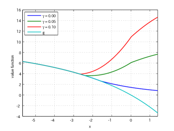
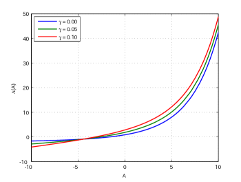
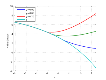
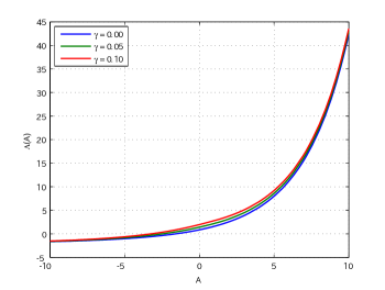
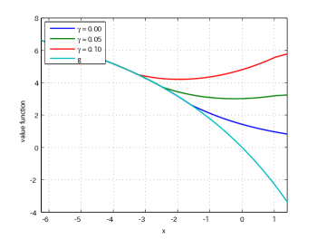
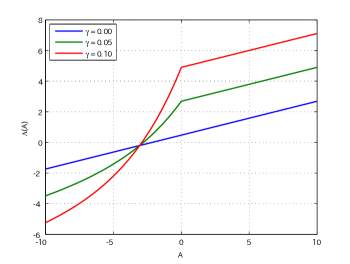
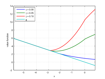
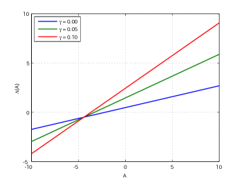
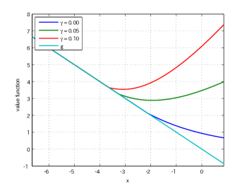
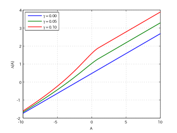
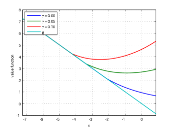
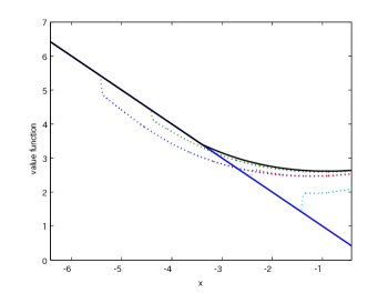
The results for (a) and (b) are graphically shown in Figures 1 and 2, respectively. In each figure, we plot the function as in (2.18) and the value function for each choice of . As can be confirmed, the function is indeed monotonically increasing and hence the unique root of can be obtained easily by the bisection method. Using these optimal threshold levels, the value functions are computed via (2.28).
We see that the value functions are differentiable even at the optimal threshold levels and this confirms the smooth fit as in Remark 2.4 because is of unbounded variation with .
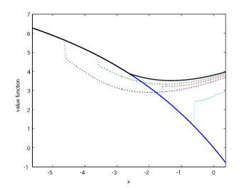
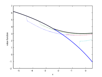
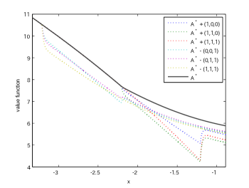
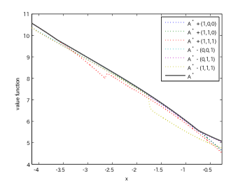
In order to verify that these are indeed optimal, we focus on the case and plot in Figure 3 the value function in comparison to the expected values of “perturbed” strategies for . Notice that these can be computed by the formula (2.27). For any choice of , it is easy to see that is continuous as in Remark 2.4 but fails to be differentiable at . We can confirm in all six cases that indeed dominates for uniformly in . This numerically verifies Propositions 2.1 and 2.2.
 |
 |
| for | value function for |
 |
 |
| for | value function for |
 |
 |
| for | value function for |
 |
 |
| for | value function for |
 |
 |
| for | value function for |
 |
 |
| for | value function for |
 |
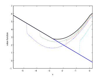 |
| (a-i) with | (b-i) with |
 |
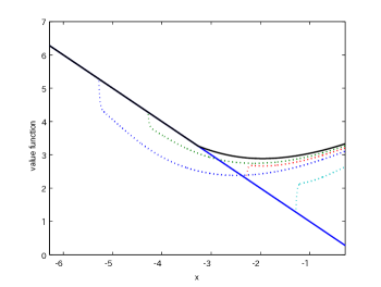 |
| (a-ii) with | (b-ii) with |
 |
 |
| (a-iii) with | (b-iii) with |
4.3. Numerical results on the multiple-stage problem
We now move onto the multiple-stage problem. We assume for brevity and use for and the functions (a)-(b) and (i)-(iii) defined for the one-stage problem.
For , we assume for some and with and a fixed value , whereas for , for some . Also, we let (i) with , , and , (ii) for and and (iii) for .
We conduct a number of experiments for various values of coefficients. By using the algorithm given in Subsection 3.2, the optimal threshold levels take values among and satisfy one of the following four cases:
-
Case 1: ;
-
Case 2: ;
-
Case 3: ;
-
Case 4: .
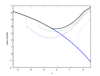
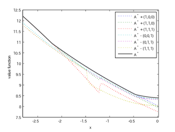
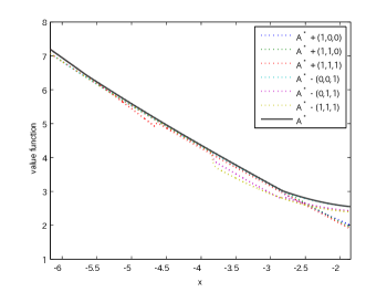
Here we use a random number generator to sample , for , , and for each until we attain each of Cases 1 to 4. The generated parameters and the corresponding threshold levels are summarized in Table 1. In order to validate the optimality of the strategy , we compare in Figure 4 the value function with those of perturbed strategies , , where
with , , , , and . It is clear that because by construction. Figure 4 suggests in all cases that the value obtained by dominates uniformly over those obtained by the perturbed strategies. These results are indeed consistent with our main theoretical results. In view of Figure 4, we also observe that there are up to three kinks (at ) in the value function although these are still differentiable. This is again due to smooth fit as in Remark 2.4. The perturbed strategies on the other hand fail to be differentiable while they are still continuous.
| Case 1 | (0.49, 0.19, 0.17, 0.03) | (0.05, 0.24, 0.46, 0.13) |
|---|---|---|
| Case 2 | (0.47, 0.17, 0.06, 0.12) | (0.24, 0.18, 0.19, 0.05) |
| Case 3 | (0.04, 0.06, 0.01, 0.12) | (0.01, 0.11, 0.26, 0.05) |
| Case 4 | (0.39, 0.28, 0.17, 0.16) | (0.06, 0.01, 0.40, 0.08) |
| Case 1 | (2.11, 2.09, 3.51, 3.49) | (4.71, 1.51, 2.70, 0.89) |
|---|---|---|
| Case 2 | (0.66, 2.88, 1.77 0.22) | (4.78, 1.17, 0.08, 3.24) |
| Case 3 | (1.84, 2.39, 4.20, 2.23) | (3.01, 3.72, 2.57, 4.20) |
| Case 4 | (3.01, 3.45, 0.42, 0.76) | (3.27, 2.25, 4.57, 2.69) |
| Case 1 | 0.9991 |
|---|---|
| Case 2 | 0.6477 |
| Case 3 | 0.6265 |
| Case 4 | 0.0782 |
| (simple) | (linear) | (exponential) | |
|---|---|---|---|
| Case 1 | 0.2920 | 0.4317 | 0.0155 |
| Case 2 | 0.4173 | 0.0497 | 0.9027 |
| Case 3 | 0.3070 | 0.0611 | 0.2195 |
| Case 4 | 0.0759 | 0.0540 | 0.5308 |
| Case 1 | -2.44 | -2.83 | -1.39 | -2.59 | -2.03 | -2.21 | -2.21 | -2.21 | -2.21 |
| Case 2 | -0.48 | -2.31 | -2.18 | -0.85 | -2.22 | -1.34 | -0.48 | -2.22 | -2.22 |
| Case 3 | -3.15 | -2.35 | -5.67 | -2.85 | -4.14 | -3.75 | -2.85 | -2.85 | -5.67 |
| Case 4 | -0.76 | -3.07 | -3.64 | -0.85 | -3.59 | -1.89 | -0.76 | -3.07 | -3.64 |
 |
 |
| Case 1 | Case 2 |
 |
 |
| Case 3 | Case 4 |
5. Concluding Remarks
In this paper, we studied a wide class of optimal stopping problems for a general spectrally negative Lévy process and extended them to multiple-stopping. Our framework is applicable to a wide range of settings particularly in real option problems where the firm withdraws from a project in stages. Our analytical results suggest that the optimal solutions can be characterized by the threshold levels that are zeros of certain monotone functions, and the corresponding value functions can be expressed in terms of the scale function. Our numerical experiments suggest, for the phase-type jump case, that these can be solved instantaneously with high precision. These tools we developed in this paper are highly valuable and can be used flexibly for analysis in real options and other fields of finance and industrial applications.
There are several directions for future research. First, our results can be pursued for a general Lévy process with both positive and negative jumps. While it makes the problem less tractable, it is expected that these can be done at least for the cases with rational forms of Wiener-Hopf factors such as meromorphic Lévy processes [23] and phase-type Lévy processes [2]. Second, by using phase-type fitting, one can approximate any Lévy process by those with phase-type jumps as in Section 4. By calibrating with real financial and industrial data as in [3], one can conduct detailed empirical analyses on optimal stopping strategies and the value functions. Finally, it is an interesting extension to consider “swing option type” multiple-stopping with refraction periods as in [11, 12] where any two consecutive stoppings must be separated by fixed constants.
Appendix A Proofs
A.1. Proof of Lemma 2.1
Let , . We have
and hence
Let , . Then,
| (A.1) |
(Case 1) First suppose for all . Simple algebra gives
| (A.2) |
where
By the definition of and , we rewrite as
where the last equality holds by (2.6). On the other hand, ; see page 213 of [24]. Hence
which shows for the case for all .
(Case 2) Suppose for some (with for by assumption). Take a sequence of (strictly) increasing sequence . Then a modification of (2.18) with replaced with is by Case 1
By the definition of as in (2.25), we have
On the other hand, in view of (A.1), its integrand is monotone in . Hence by the monotone convergence theorem and because and are continuous in , , and the proof is complete for Case 2.
A.2. Proof of Lemma 2.2
Because is infinitely differentiable, the results are clear for . Hence we show for . Because is differentiable on as in Remark 2.1(1), is twice differentiable.
Regarding , integration by parts thanks to the continuity of gives (with , )
It is differentiable with
When is of unbounded variation, because as in Remark 2.1(2), is twice-differentiable with
A.3. Proof of Proposition 2.1
(i) Suppose . By directly using the results of [17] (Lemma 3.7 and Proposition 3.4), we obtain
| (A.3) | ||||
where is the infinitesimal generator of applied to a sufficiently smooth function , i.e.,
Lemma A.1.
If , we have on .
Proof.
Fix . First, if we define , ,
By the definition of , if we define , ,
for any and hence we have
| (A.4) |
By how is chosen,
| (A.5) |
Because is increasing and
| (A.6) |
By and ,
It is also easy to see that
| (A.7) |
Indeed, for the case , we must have and hence (A.7) holds by ; for the case , the left-hand side is positive while the right-hand side is negative in (A.7); for the case , the left-hand side is positive because is, while the right-hand side is zero. Hence, by (A.5)-(A.7), holds.
This result also holds for the case . In this case, , for any . Therefore holds by the same reasoning as in (1) by simply replacing with for any .
∎
We are now ready to verify the optimality of for the case . Thanks to Lemma 2.2 and the continuous/smooth fit condition as in Remark 2.4, a version of Meyer-Ito’s formula as in Theorem IV.71 of [32] (see also Theorem 2.1 of [30]) implies
with the local martingale part
where is the Poisson random measure associated with the dual process .
Fix any stopping time , and define for each the stopping time as
and the martingale process , with . By optional sampling and because via (A.3) and Lemma A.1,
When , (the same result holds for by Remark 2.3). On the other hand, if and , because on , the value is bounded from below by a limit:
Hence,
where the last equality holds by monotone convergence applied to the term and because on , which is bounded because is decreasing. Because is increasing, the expectation on the right hand side decreases in and hence
In sum, is bounded from above. Recall also Remark 2.2. Hence, Fatou’s lemma gives upon and
Finally, (A.3) shows the result for .
(ii) It is now left to show for the case . Because for any as in (2.20), there again exists . Assumption 2.2 guarantees that ; see e.g., [34]. Because the slope of is bounded on the half-line, this shows that
This together with Remark 2.2 shows that has the desired expression.
Because for any , for any (hence the stopping region is an empty set). Moreover, because is attained by , we have the claim.
A.4. Proof of Proposition 2.2
(1,2) We first suppose . Then by definition . Because for any , it is sufficient to show for . This is indeed so because by (2.17), (2.20) and due to ,
This proves (2). For (1), we additionally show for the case . By (2.20), for any . For , and by (2.17), (2.20) and due to ,
Therefore uniformly in , as desired.
The corresponding value function (for (1)) can be expressed as the sum of (2.15):
From the definition of that makes (2.18) vanish, it is simplified to
as desired.
(3) The proof is the same as that of Proposition 2.1(3).
References
- [1] L. Alili and A. E. Kyprianou. Some remarks on first passage of Lévy processes, the American put and smooth pasting. Ann. Appl. Probab., 15:2062–2080, 2004.
- [2] S. Asmussen, F. Avram, and M. R. Pistorius. Russian and American put options under exponential phase-type Lévy models. Stochastic Process. Appl., 109(1):79–111, 2004.
- [3] S. Asmussen, D. Madan, and M. R. Pistorius. Pricing equity default swaps under an approximation to the CGMY Lévy model. J. Comput. Financ., 11(2):79–93, 2007.
- [4] F. Avram, A. E. Kyprianou, and M. R. Pistorius. Exit problems for spectrally negative Lévy processes and applications to (Canadized) Russion options. Ann. Appl. Probab., 14:215–235, 2004.
- [5] F. Avram, Z. Palmowski, and M. R. Pistorius. On the optimal dividend problem for a spectrally negative Lévy process. Ann. Appl. Probab., 17(1):156–180, 2007.
- [6] E. Baurdoux and A. E. Kyprianou. The McKean stochastic game driven by a spectrally negative Lévy process. Electron. J. Probab., 13:no. 8, 173–197, 2008.
- [7] E. Baurdoux and A. E. Kyprianou. The Shepp-Shiryaev stochastic game driven by a spectrally negative Lévy process. Theory Probab. Appl., 53, 2009.
- [8] J. Bertoin. Exponential decay and ergodicity of completely asymmetric Lévy processes in a finite interval. Ann. Appl. Probab., 7(1):156–169, 1997.
- [9] S. Boyarchenko and S. Levendorskiĭ. Irreversible decisions under uncertainty, volume 27 of Studies in Economic Theory. Springer, Berlin, 2007.
- [10] S. Boyarchenko and S. Z. Levendorskiĭ. General option exercise rules, with applications to embedded options and monopolistic expansion. Contrib. Theor. Econ., 6:Art. 2, 53 pp. (electronic), 2006.
- [11] R. Carmona and S. Dayanik. Optimal multiple stopping of linear diffusions. Math. Oper. Res., 33(2):446–460, 2008.
- [12] R. Carmona and N. Touzi. Optimal multiple stopping and valuation of swing options. Math. Finance, 18(2):239–268, 2008.
- [13] T. Chan, A. Kyprianou, and M. Savov. Smoothness of scale functions for spectrally negative Lévy processes. Probab. Theory Relat. Fields, 150:691–708, 2011.
- [14] A. Deaton and G. Laroque. On the behaviour of commodity prices. Rev. Econ. Stud., 59:1–23, 1992.
- [15] A. Dixit and R. Pindyck. Investment under Uncertainty. Princeton University Press, 1996.
- [16] E. Egami, T. Leung, and K. Yamazaki. Default swap games driven by spectrally negative Lévy processes. Stochastic Process. Appl., 123(2):347–384, 2013.
- [17] M. Egami and K. Yamazaki. On the continuous and smooth fit principle for optimal stopping problems in spectrally negative levy models. Adv. in Appl. Probab., 46(1).
- [18] M. Egami and K. Yamazaki. Precautional measures for credit risk management in jump models. Stochastics, 85(1):111–143, 2013.
- [19] M. Egami and K. Yamazaki. Phase-type fitting of scale functions for spectrally negative Lévy processes. J. Comput. Appl. Math., 264:1–22, 2014.
- [20] A. Feldmann and W. Whitt. Fitting mixtures of exponentials to long-tail distributions to analyze network performance models. Perform. Evaluation, (31):245–279, 1998.
- [21] D. Hernandez-Hernandez and K. Yamazaki. Games of singular control and stopping driven by spectrally one-sided Lévy processes. Stochastic Process. Appl., forthcoming.
- [22] A. Kuznetsov, A. Kyprianou, and V. Rivero. The theory of scale functions for spectrally negative Lévy processes. Springer Lecture Notes in Mathematics, 2061:97–186, 2013.
- [23] A. Kuznetsov, A. E. Kyprianou, and J. C. Pardo. Meromorphic Lévy processes and their fluctuation identities. Ann. Appl. Probab., 22:1101–1135, 2012.
- [24] A. E. Kyprianou. Introductory lectures on fluctuations of Lévy processes with applications. Universitext. Springer-Verlag, Berlin, 2006.
- [25] A. E. Kyprianou and B. A. Surya. Principles of smooth and continuous fit in the determination of endogenous bankruptcy levels. Finance Stoch., 11(1):131–152, 2007.
- [26] H. E. Leland. Corporate debt value, bond covenants, and optimal capital structure. J. Finance, 49(4):1213–1252, 1994.
- [27] H. E. Leland and K. B. Toft. Optimal capital structure, endogenous bankruptcy, and the term structure of credit spreads. J. Finance, 51(3):987–1019, 1996.
- [28] T. Leung and K. Yamazaki. American step-up and step-down default swaps under Lévy models. Quant. Finance, 13(1):137–157, 2013.
- [29] E. Mordecki. Optimal stopping and perpetual options for Lévy processes. Finance Stoch., 6:473–493, 2002.
- [30] B. Øksendal and A. Sulem. Applied Stochastic Control of Jump Diffusions. Springer, New York, 2005.
- [31] G. Peskir and A. N. Shiryaev. Optimal stopping and Free-Boundary Problems (Lectures in Mathematics, ETH Zürich). Birkhauser, Basel, 2006.
- [32] P. Protter. Stochastic integration and differential equations. Springer, 2005.
- [33] B. A. Surya. Evaluating scale functions of spectrally negative Lévy processes. J. Appl. Probab., 45(1):135–149, 2008.
- [34] K. Yamazaki. Inventory control for spectrally positive Lévy demand processes. arXiv:1303.5163, 2013.
- [35] S.-R. Yang and B. W. Brorsen. Nonlinear dynamics of daily cash prices. Amer. J. Agr. Econ., 74(3):706–715, 1992.