Internal and External Fluctuation Activated Non-equilibrium Reactive Rate Process

Abstract

The activated rate process for non-equilibrium open systems is studied taking into account both internal and external noise fluctuations in a unified way. The probability of a particle diffusing passing over the saddle point and the rate constant together with the effective transmission coefficient are calculated via the method of reactive flux. We find that the complexity of internal noise is always harmful to the diffusion of particles. However the external modulation may be beneficial to the rate process.

I INTRODUCTION

More than seventy years ago H. A. Kramers published a seminal work on the diffusion model of chemical reactions kramers . Ever since then, the theory of activated processes has become a central issue in many fields of study aps1 ; aps2 , notably in chemical physics, nonlinear optics and condensed matter physics. In the model, the particle was supposed to be immersed in a huge equilibrium medium so that it can gain enough energy to cross the barrier from its thermally activation. The common feature of an overwhelming majority of such treatments is that the system is thermodynamically closed. That is to say, the noise of the medium is of internal origin so that the dissipation-fluctuation theorem fdt1 ; fdt2 is satisfied and a zero current steady state situation is characterized by an equilibrium Boltzmann distribution.

However, when the system is thermodynamically open, for example, driven by an external noise which is independent of the medium whor , no relation between the dissipation and fluctuations can be dependent on. The corresponding situation aforesaid, if attainable, can then only be defined by a steady state condition dsray2 ; dsray3 which may depend not only on the strength and correlation of the external noise but also on the dissipation of the system. The external noise will modify the dynamics of activation in the region around the barrier top so that an unusual effective stationary flux across it gets resulted. This would in no doubt induce an unfamiliar activated barrier escaping process that is worth pursuing for the rate theory.

Therefore we present in this paper a recent study of us on the activated rate process where the diffusing particle is under the joint influence of the internal noise combining an external one. The paper is organized as follows: In Sec. II, reactive dynamics at the barrier top is investigated by analytically solving the generalized Langevin equation. In Sec. III, we give a detailed discussion about the combined effect of internal and external noises on the rate process by asymptotically calculating the rate function and its transmission coefficient. Sec. IV serves as a summary of our conclusion where some implicate applications of this study are also discussed.

II Reactive dynamics at the barrier top

We consider the motion of a particle of unit mass moving in a Kramers type potential $U(x)$ such that it is acted upon by random forces $\zeta(t)$ and $\epsilon(t)$ of both internal and external origin, respectively, in terms of the following generalized Langevin equation (GLE):

$$\ddot{x}+\int^{t}_{0}dt^{\prime}\gamma(t-t^{\prime})\dot{x}(t^{\prime})+\partial_{x}U(x)=\zeta(t)+\epsilon(t),$$ (1)

where $U(x)$ is the potential, the friction kernel $\gamma(t)$ is connected to internal noise by the well-known fluctuation-dissipation theorem (FDT) fdt1 ; fdt2 $\langle\zeta(t)\zeta(t^{\prime})\rangle=k_{B}T\gamma(t-t^{\prime})$. Both the noises $\zeta(t)$ and $\epsilon(t)$ are assumed stationary and Gaussian with arbitrary decaying type of correlation. We further assume, without any loss of generality, that $\zeta(t)$ is independent of $\epsilon(t)$ so that we have $\langle\zeta(t)\epsilon(t^{\prime})\rangle=0$ and $\langle\epsilon(t)\epsilon(t^{\prime})\rangle_{e}=2D\psi(t-t^{\prime})$. Here $\langle\cdots\rangle_{e}$ implies the averaging over all the realizations of $\epsilon(t)$ with $D$ the intensity constant and $\psi(t)$ a relevant memory function. In other words, the external noise is independent of the friction kernel $\gamma(t)$ and so there is no corresponding fluctuation-dissipation relation. However, correlation $\langle\epsilon(t)\epsilon(t^{\prime})\rangle_{e}=2D\psi(t-t^{\prime})$ is reminiscent of the familiar FDT formula due to the appearance of the external noise intensity, it serves rather as a thermodynamic consistency condition instead.

Due to the Gaussian property of the noises $\zeta(t)$ and $\epsilon(t)$ and the linearity of the GLE, the joint probability density function of the system oscillator must still be written in a Gaussian form adelm The reduced distribution function can then be yielded by integrating out all the variants except $x$ as

$$W(x,t;x_{0},v_{0})=\frac{1}{\sqrt{2\pi}\sigma_{x}(t)}\textrm{exp}\left[{-\frac{(x-\langle x(t)\rangle)^{2}}{2\sigma^{2}_{x}(t)}}\right].$$ (2)

in which the average position $\langle x(t)\rangle$ and variance $\sigma^{2}_{x}(t)$ can be obtained by Laplace solving the GLE. In the case of an inverse harmonic potential $U(x)=-\frac{1}{2}m\omega^{2}_{b}x^{2}$, it reads

$$\langle x(t)\rangle = \left[1+\omega^{2}_{b}\int^{t}_{0}H(t^{\prime})dt^{\prime}\right]x_{0}+H(t)v_{0}$$ (3a)

$$\sigma^{2}_{x}(t) = \int^{t}_{0}dt_{1}H(t-t_{1})\int^{t_{1}}_{0}dt_{2}\langle\xi(t_{1})\xi(t_{2})\rangle H(t-t_{2})$$ (3b)

where $H(t)$ namely the response function can be yielded from inverse Laplace transforming $\hat{H}(s)=[s^{2}+s\hat{\gamma}(s)-\omega^{2}_{b}]^{-1}$ with residue theorem ret1 ; ret2 . $\xi(t)$ $(=\zeta(t)+\varepsilon(t))$ is an effective noise of zero mean $\langle\xi(t)\rangle=0$ whose correlation is given by

$$\langle\xi(t)\xi(t^{\prime})\rangle=\langle\zeta(t)\zeta(t^{\prime})\rangle+\langle\epsilon(t)\epsilon(t^{\prime})\rangle_{e},$$ (4)

where the two averages in the right hand side are taken independently.

The probability of passing over the saddle point, namely also the characteristic function which is crucial for the activated barrier crossing process, can then be determined mathematically by integrating Eq.(2) over $x$ from zero to infinity as

$$P(x_{0},v_{0};t) = \int^{\infty}_{0}W(x,t;x_{0},v_{0})dx,$$ (5)

$$= \frac{1}{2}\textrm{erfc}\left[-\frac{\langle x(t)\rangle}{\sqrt{2}\sigma_{x}(t)}\right],$$

The escape rate of a particle, defined in the spirit of reactive flux method by assuming the initial conditions to be at the top of the barrier, can then be yielded from

$$k(t) = \frac{1}{h}\int^{\infty}_{-\infty}dx_{0}\int^{\infty}_{-\infty}v_{0}W_{\textrm{st}}(x_{0},v_{0})P(x_{0},v_{0};t)\delta(x_{0}-x_{b})dv_{0}$$ (6)

in the phase space. This in proceeding results in a generalized transition state (TST) rate TST1 ; TST2 ; TST3 : $k^{\textrm{TST}}=\frac{1}{Qh}e^{-U_{b}/(D_{b}+\Psi(\infty))}$ and an effective transmission factor

$$\kappa(t) = \left(1+\frac{\sigma^{2}_{x}(t)}{D_{b}H^{2}(t)}\right)^{-1/2},$$ (7)

where $W_{\textrm{st}}(x_{0},v_{{}_{0}})=\frac{1}{Q}\textrm{exp}[-\{{\frac{v_{0}^{2}}{2D_{b}}+\frac{\tilde{U}(x_{0})}{D_{b}+\Psi(\infty)}}\}]$ is a Boltzmann form stationary probability distribution which can be obtained from the steady state Fokker-Planck equation dsray3 . This stationary distribution for the non-equilibrium open system is not an equilibrium distribution but it plays the role of an equilibrium distribution of the closed system, which may, however, be recovered in the absence of the external noise. $(D_{b}+\Psi(\infty))/k_{B}$ in the exponential factor of $k^{\textrm{TST}}$ defines a new effective temperature characteristic of the steady state of the non-equilibrium open system.

In the particular case we have considered, parameters used heretofore are defined as dsray2 ; dsray3 : $\tilde{U}(x)=U_{b}-\frac{1}{2}\Omega_{b}^{2}(x-x_{b})^{2}$ the renormalized linear potential near the barrier top with $\Omega_{b}$ an effective frequency and $U_{b}$ the barrier height. $\Psi(\infty)$ and $D_{b}=\Phi(\infty)/\Gamma(\infty)$ are to be calculated from

$$\Phi(t) = \Omega_{b}^{2}(t)\sigma^{2}_{xv}(t)+\Gamma(t)\sigma^{2}_{v}(t)+\frac{1}{2}\frac{d}{dt}\sigma^{2}_{xv}(t),$$ (8a)

$$\Psi(t) = \frac{d}{dt}\sigma^{2}_{xv}(t)+\Gamma(t)\sigma^{2}_{xv}(t)+\Omega_{b}^{2}(t)\sigma^{2}_{x}(t)-\sigma^{2}_{v}(t),$$ (8b)

for the steady state in which $\Gamma(t)=-\frac{d}{dt}\textrm{ln}\Lambda(t)$, $\Omega_{b}^{2}(t)=\dot{H}(t)(\dot{H}(t)-H(t))/\Lambda(t)$ and $\Lambda(t)=\frac{\dot{H}(t)}{\omega_{b}^{2}}[1-\omega_{b}^{2}\int_{0}^{t}d\tau H(\tau)]+H^{2}(t)$. Other variances besides $\sigma^{2}_{x}(t)$ are also to be got from Laplace solving the GLE. These variables will play a decisive role in the calculation of barrier escaping rate. Therefore, in general, one has to work out these quantities first for analytically tractable models adelm .

As is expected, all the parameters besides the rates $\kappa(t)$ and $k(t)$ are closely related to the internal and external noises. Therefore a combining control of internal and external noise on the activated barrier escaping process is prospected. This is what will be involved in the following sections.

III Internal vs external noise

Before accomplishing the following calculations, let us firstly digress a little bit about $P(x_{0},v_{0};t)$ and $\kappa(t)$ which are the central results of this study. As has been shown in Eqs. (5) and (7), both the expressions of $P(x_{0},v_{0};t)$ and $\kappa(t)$ are reminiscent of the familiar previous results jcp ; jdb . Although variance $\sigma^{2}_{x}(t)$ has been changed intrinsically by the external noise, difference lives only superficially in the emergence of $D_{b}$ which is an asymptotical constant in the long time limit. Due to the independence of internal and external noises, other variances such as $\langle x(t)\rangle$ and $H(t)$ depend only on the internal noise. Therefore, from the viewpoint of diffusing passing over the saddle point, the mean position of the Gaussian packet relies simply on the internal noise while the width of it depends not only on the internal noise but also on the external one. It is the combining effect of internal and external noise that determines the final diffusing process. In what follows, it shall be concerned with several limiting situations to illustrate the general result systematically for both thermal and non-thermal activated processes.

III.1 Internal white noise

Firstly we consider the simplest case of a $\delta$ correlated internal thermal noise combining with no external ones. To this end, it is to set

$$\epsilon(t)=0\hskip 14.22636pt\textrm{and}\hskip 14.22636pt\langle\zeta(t)\zeta(t^{\prime})\rangle=k_{B}T\gamma\delta(t-t^{\prime}).$$ (9)

By combining with the abbreviations in Eqs.(3) and (8), all the quantities we need for the activated process can be obtained easily. After some algebra it follows that

$$\Psi(\infty)=0\hskip 14.22636pt\textrm{and}\hskip 14.22636ptD_{b}=k_{B}T.$$ (10)

The relations obtained heretofore reduce to the general form

$$\kappa(t) = \left(1+\frac{\sigma^{2}_{x}(t)}{k_{B}TH^{2}(t)}\right)^{-1/2}.$$ (11)

This is a trivial result for the one-dimensional time-dependent barrier passage jdb . It generally describes the possibility of a particle already escaped from the metastable well to recross the barrier. In the case of no external noise modulation, it keeps its usual form just as it should be.

III.2 Internal color noise

Next we discuss the case of purely internal color noise. For example, we set the internal noise to be Ornstein-Uhlenbeck (OU) type ou1 ; ou2 . That is

$$\epsilon(t)=0\hskip 14.22636pt\textrm{and}\hskip 14.22636pt\langle\zeta(t)\zeta(t^{\prime})\rangle=k_{B}T\frac{G}{\tau_{c}}e^{-|t-t^{\prime}|/\tau_{c}},$$ (12)

where $G$ denotes the strength while $\tau_{c}$ refers to the correlation time of the noise. It should be noted that for $\tau_{c}\rightarrow 0$ the internal noise shown above becomes also $\delta$ correlated. After some algebra we can obtain from Eqs.(3) and (8) again that

$$\Psi(\infty)=k_{B}T\left(\frac{\Omega_{b}^{2}}{\omega_{b}^{2}}-1\right)\hskip 14.22636pt\textrm{while}\hskip 14.22636ptD_{b}=k_{B}T.$$ (13)

This will result in a different form of TST rate $k^{\textrm{TST}}$ but has no influence on the form of transmission coefficient $\kappa(t)$. However, since in most cases $\Omega_{b}^{2}\cong\omega_{b}^{2}$, the value of $\Psi(\infty)$ is actually close to 0. The values of variance $\sigma^{2}_{x}(t)$ and $H(t)$ are also changed intrinsically. Therefore, although the form of $\kappa(t)$ has not been changed, the rate process has been modified implicitly due to the alteration of internal noise.

III.3 Internal and external white noise

In further, let us turn to investigate the more complicated combining case where both the internal and external noise to be $\delta$ correlated, i.e.

$$\langle\epsilon(t)\epsilon(t^{\prime})\rangle_{e}=2\mathcal{D}\delta(t-t^{\prime})\hskip 14.22636pt\textrm{and}\hskip 14.22636pt\langle\zeta(t)\zeta(t^{\prime})\rangle=k_{B}T\gamma\delta(t-t^{\prime}).$$ (14)

in which $\mathcal{D}$ is the strength of the external white noise. This may be the simplest combining case of internal and external noise. Derive again from the abbreviations heretofore we obtain

$$\Psi(\infty)=0\hskip 14.22636pt\textrm{and}\hskip 14.22636ptD_{b}=k_{B}T+\frac{\mathcal{D}}{\gamma}.$$ (15)

Noticing that comparing with the aforesaid case in Sec.III.1 a new effective temperature due to external noise is defined here by $\mathcal{D}/(\gamma k_{B})$ eft . But in the limit of $\mathcal{D}\rightarrow 0$, the previous one-dimensional form of $\kappa(t)$ for pure internal white noise can still be recovered by Eq.(7). However, the rate process has also been changed intrinsically due to the effect of external noise.

III.4 Internal color and external white noise

Finally, we consider a particular case where the external noise is $\delta$ correlated while the internal is an OU process, i.e.,

$$\langle\epsilon(t)\epsilon(t^{\prime})\rangle_{e}=2\mathcal{D}\delta(t-t^{\prime})\hskip 14.22636pt\textrm{and}\hskip 14.22636pt\langle\zeta(t)\zeta(t^{\prime})\rangle=k_{B}T\frac{G}{\tau_{c}}e^{-|t-t^{\prime}|/\tau},$$ (16)

both symmetric with respect to the time argument and assumed to be uncorrelated with each other. By virtue of similar derivations as heretofore, we find it is difficult to get an explicitly simple expression of $\Psi(\infty)$ while $D_{b}=k_{B}T$ is recovered again. This is nontrivial in the presence of external noise because it seems as if there is not any effect on the rate process that comes from the external noise. But actually all the effects have been contained in the calculations of $\sigma^{2}_{x}(t)\rangle$ and $H(t)$ so as in that of $\kappa(t)$.

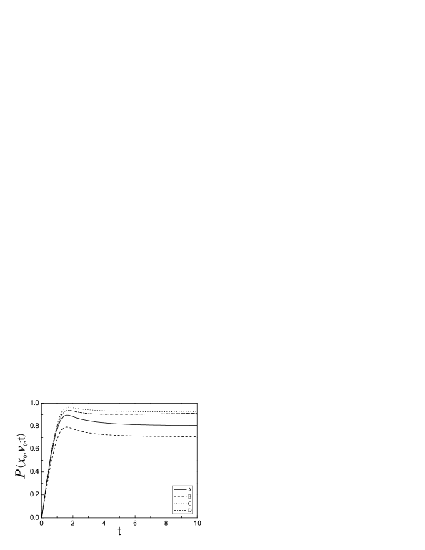
Figure 1: Instantaneous values of $\chi(x_{0},v_{0};t)$ and $\kappa(t)$ for various types of internal and external noise combinations. Dimensionless parameters used are $\gamma=4.0$, $\omega_{b}=1.0$, $G=3.0$ and $\tau=0.3$. Particles are assumed to start from position $x_{0}=-1.0$ with initial velocity $v_{0}=6.0$. Lines signed as $A$, $B$, $C$, $D$ represent the different cases discussed in the corresponding subsections respectively.

In order to give an explicit revelation of the combining effect of the noises on the rate process, we plot in Fig.1 the instantaneous values of $P(x_{0},v_{0};t)$ and $\kappa(t)$ at different types of combining cases aforesaid. From which we can see that the asymptotic stationary value of $P(x_{0},v_{0};t)$ and $\kappa(t)$ (defined as $P_{\textrm{st}}$ and $\kappa_{\textrm{st}}$ respectively) in the internal color case is smaller than that of internal white case no matter the system is modulated by an external white noise or not. On the contrary, both $P_{\textrm{st}}$ and $\kappa_{\textrm{st}}$ are larger than those of pure internal case supposing an external noise is set on with modulation. Thus we can infer from considering the intrinsic meaning of $P(x_{0},v_{0};t)$ and $\kappa(t)$ that the complexity of internal noise (or dissipation) is always harmful to the diffusion of particles. However the external modulation may be beneficial to the rate process. This is a non-trivial result of great meaning to many different kinds of realistic situations in forming a non-equilibrium (or non-thermal) system-reservoir coupling environment phys1 ; phys2 .

IV Summary and discussion

In summary, we have studied in this paper the activated rate process for non-equilibrium open systems taking into account both internal and external noise fluctuations in a unified way. We calculated the probability of a particle diffusing passing over the saddle point and the rate constant together with the effective transmission coefficient via the method of reactive flux. The combining control of internal and external noises on the activated barrier escaping process is investigated. We find that the complexity of internal noise is always harmful to the diffusion of particles. However the external modulation may be beneficial to the rate process.

We believe that these considerations are likely to be important in other related issues in non-equilibrium open systems and may serve as a basis for studying processes occurring within irreversibly driven environments jray ; rher and for thermal ratchet problems rdas . The externally generated non-equilibrium fluctuations can bias the Brownian motion of a particle in an anisotropic medium and may also be used for designing molecular motors and pumps.

References

- (1) H. A. Kramers, Physica (Utrecht) 7, 284 (1940).
- (2) P. Hänggi, P. Talkner, and M. Borkovec, Rev. Mod. Phys. 62, 251 (1990).
- (3) V. I. Melnikov, Phys. Rep. 209, 1 (1991).
- (4) R. Kubo, Rep. Prog. Phys. 29, 255 (1966).
- (5) R. Kubo, M. Toda and N. Hashitsume, Statistical Physics II: Nonequilibrium Statistical Mechanics (Springer-Verlag, New York, 1985).
- (6) W. Horsthemke and R. Lefever, Noise-Induced Transitions (Springer-Verlag, Berlin, 1984).
- (7) S. K. Banik, J. R. Chaudhuri, and D. S. Ray, J. Chem. Phys. 112, 8330 (2000).
- (8) J. R. Chaudhuri, S. K. Banik, B. C. Chandra and D. S. Ray, Phys. Rev. E 63, 061111 (2001).
- (9) S. A. Adelman, J. Chem. Phys. 64, 124 (1976).
- (10) J. H. Mathews and R. W. Howell, Complex Analysis: for Mathematics and Engineering, 5th Ed. (Jones and Bartlett Pub. Inc. Sudbury, MA, 2006).
- (11) R. Muralidhar, D. J. Jacobs, D. Ramkrishna and H. Nakanishi, Phys. Rev. A 43, 6503 (1991).
- (12) T. Seideman and W. H. Miller, J. Chem. Phys. 95, 1768 (1991).
- (13) J. M. Sancho, A. H. Romero and K. Lindenberg, J. Chem. Phys. 109, 9888 (1998).
- (14) E. Pollak and M. S. Child, J. Chem. Phys. 72, 1669 (1980).
- (15) C. Y. Wang, J. Chem. Phys. 131, 054504 (2009).
- (16) J. D. Bao, J. Chem. Phys. 124, 114103 (2006).
- (17) G. E. Uhlenbeck and L. S. Ornstein, Phys. Rev. 36, 823 (1930).
- (18) M. C. Wang and G. E. Uhlenbeck, Rev. Mod. Phys. 17, 323 (1945).
- (19) J. M. Bravo, R. M. Velasco and J. M. Sancho, J. Math. Phys. 30, 2023 (1989).
- (20) F. Moss and P. V. E. McClintock, Noise in Nonlinear Dynamical Systems (Cambridge University, England, 1989).
- (21) W. Horsthemke and R. Lefever, Noise-Induced Transitions (Springer-Verlag, Berlin, 1984).
- (22) J. Ray Chaudhuri, G. Gangopadhyay and D. S. Ray, J. Chem. Phys. 109, 5565 (1998).
- (23) R. Hernandez, J. Chem. Phys. 111, 7701 (1999).
- (24) R. D. Astumian, Science 276, 917 (1997), and the references given therein.