A numerical technique for studying topological effects on the thermal properties of knotted polymer rings

Abstract

The topological effects on the thermal properties of several knot configurations are investigated using Monte Carlo simulations. In order to check if the topology of the knots is preserved during the thermal fluctuations we propose a method that allows very fast calculations and can be easily applied to arbitrarily complex knots. As an application, the specific energy and heat capacity of the trefoil, the figure-eight and the $8_{1}$ knots are calculated at different temperatures and for different lengths. Short-range repulsive interactions between the monomers are assumed. The knots configurations are generated on a three-dimensional cubic lattice and sampled by means of the Wang-Landau algorithm and of the pivot method. The obtained results show that the topological effects play a key role for short-length polymers. Three temperature regimes of the growth rate of the internal energy of the system are distinguished.

I Introduction

Topological polymers are a fascinating subject by themselves. Moreover, the interest in this topic is motivated by possible industrial applications, for example because knots in polymer materials are able to influence the viscoelastic properties grosberg , and due to their relevance in biology and biochemistry, see for instance dna ; katritch96 ; katritch97 ; krasnow ; laurie ; cieplak ; liu ; wasserman ; sumners . Polymer rings may be found in nature or in artificial materials in the form of knots that can be additionally linked together. In this work we explore the case of the statistical mechanics of a single polymer knot. Various topological configurations are taken into account: The unknot, denoted according to the Alexander-Briggs notation $0_{1}$, the trefoil $3_{1}$, the figure-eight $4_{1}$ and the knot $8_{1}$. In particular, we study the thermal properties of the above knots by computing numerically their internal energy and heat capacities. The most important problem of numerical simulations of polymer knots is to preserve their topology while their configurations are fluctuating randomly. To this purpose, several methods have been developed vologodski ; orlandini ; kurt ; mehran ; pp2 ; metzler ; muthu . Most of them, are based on the Alexander or Jones polynomials, which are rather powerful topological invariants able to distinguish with a very high degree of accuracy the different topological configurations. The main drawback of these polynomials is that their calculation is very expensive and time consuming from the computational point of view.

Here we propose a new strategy that consists in the following. First, we apply the pivot algorithm to change a given knot configuration. Starting from a seed knot, for instance those given in ref. scharein , we change it at randomly chosen points by applying the pivot algorithm pivot . After each pivot move, the difference between the old and new configurations forms a closed loop. Around it, an arbitrary surface is stretched, whose boundary is the closed loop itself. The criterion to reject changes that destroy the topology of the knot is the presence or not of lines of the old knot that cross such surface. If these lines are present, the trial pivot move is rejected. This combination of pivot algorithm and excluded area (PAEA) provides an efficient and fast way to preserve the topology that can be applied to any knot configuration, independently of its complexity. For pivot moves involving a small number of segments the method becomes exact. This technique may be employed in the study of the thermal and mechanical properties of polymer knots. Here we have limited ourselves to the computation of the internal energy and heat capacity in the case in which the monomer interactions are of very short range, but the extension to any other interactions or to the calculations of more complicated physical quantities is possible. The configurations of the unknot, trefoil, figure-eight and $8_{1}$ knot are modeled on a cubic lattice. The sampling of the canonical ensemble is achieved by using the Wang-Landau algorithm wanglaudau at different temperatures.

The rest of this paper is organized as follows. In Sec. II, we describe the sampling and simulation methods of the polymer knots. Our strategy to distinguish possible violations of the topology of a given knot after a random change of its trajectory is explained. The calculation of the specific energy and the specific heat capacity for various polymer topologies and for different polymer lengths is presented in section III. In section IV we draw our conclusions and discuss the open problems together with new possible directions of our research.

II Model and Computational method

In the current work, we will study the topological effects on the thermal properties of polymer rings. Four types of polymers will be considered on a 3-dimensional cubic lattice, namely the unknot ${\cal U}$, the trefoil ${\cal T}$, the figure-eight ${\cal F}$ and the knot $8_{1}$, see Fig. 1.

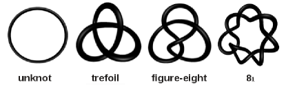
Figure 1: In this work different knot types will be studied, namely the unknot, the trefoil, the figure-eight and the $8_{1}$ knot.

A general knot will be denoted with the symbol ${\cal K}$. To simulate the trivial polymer ring ${\cal U}$, we generate a loop starting from a random point and performing a self-avoiding walk on the cubic lattice. The walk is stopped when it crosses itself, forming a loop. We generate many loops of this kind and we retain only those with a given length $L$. For nontrivial topologies, we choose a different strategy. We begin from a seed conformation and then we act repeatedly on it with the pivot method pivot to get random conformations. The elements of the loop that will be changed by the pivot move have a fixed number of segments $N=4$ or $N=5$. The elements begin at a random point in the knot, let’s say $N_{0}$ and end up at the point number $N_{0}+4$, or $N_{0}+5$. $N_{0}$ can range from 0 to $L-N$ ($L$ is the length of the polymer). We check the topology of the configuration after every pivot move, to be sure that the move will not change the topology of the given knot. Usually, this check is achieved by projecting the knot along some direction on a two dimensional plane and the relative Alexander polynomial is computed. This method has been pioneered in refs. vologodski . Here we choose another strategy, namely on a given knot ${\cal K}$ we perform a pivot move. In that way a new knot ${\cal K}^{\prime}$ is obtained. A schematic picture of the situation can be found in fig. 2. In order to verify that the topology of the knot has not been changed by the pivot move, we check that no lines of ${\cal K}$ cross the area spanned by the small loop $\Delta{\cal K}={\cal K}^{\prime}-{\cal K}$ including its border. Otherwise, this could imply that a crossing of the lines of ${\cal K}$ has happened. The definition of the area of $\Delta{\cal K}$ in a numerical simulation is a difficult problem of computer graphics. However, if the number of segments involved in the pivot moves is small, it is possible to classify all the geometries of $\Delta{\cal K}$ and to stretch a suitable surface $\Sigma_{\Delta\cal K}$ around $\Delta{\cal K}$. Next, these data, namely all geometries of $\Delta{\cal K}$ and the coordinates of the relative surfaces $\Sigma_{\Delta\cal K}$, are supplied to the code, which will then be able to detect the occurrence of possible lines of ${\cal K}$ crossing $\Sigma_{\Delta\cal K}$ or the part of its border $\Delta{\cal K}-{\cal K}\bigcap\Delta{\cal K}$, see fig. 2 for a schematic representation of what these symbols mean. If these lines are present, the trial pivot move is rejected.

Figure 2: This figure represents in a schematic way the meaning of the symbols used to denote the element ${\cal K}\bigcap\Delta{\cal K}$ of $\Delta{\cal K}$ shared with the knot $\cal K$ and the element $\Delta{\cal K}-{\cal K}\bigcap\Delta{\cal K}$ of $\Delta{\cal K}$ which is not shared with $\cal K$.

Let us note that the strategy described above could be considered as an implementation of the topological constraints based on the Gauss linking number modified to cope with the present situation, in which the Gauss linking number becomes not suitable because $\cal K$ and $\Delta\cal K$ share part of their trajectories. While the Gauss linking number is a weak topological number, our method turns out to be very efficient when applied to pivot modes with segment lengths $N=4$ and $N=5$. In both cases the geometry of the loop $\Delta\cal K$ is simple enough, that it is possible to analyze all situations in which the crossings of lines could violate the topology of $\cal K$ and to provide an exact criterion for preserving this topology without increasing exceedingly the simulation time. Only when $N>5$ it may occur that the trajectory of the old knot crosses the area $\Sigma_{\Delta\cal K}$ an even number of times. In this case, due to limitations similar to those of the Gauss linking number, allowed moves can be rejected. If this happens very frequently, the computational time may increase. However, this is not a serious drawback because the above procedure of detecting topology changes is extremely time efficient. The necessary cpu time depends essentially only on the number of segments $L$, independently on the complexity of the knot. In the following, we will restrict ourselves to the cases $N=4$ and $N=5$.
In order to calculate the internal energy of the polymer per unit of length $\langle E(\beta)\rangle/L$, where $\beta=T^{-1}$ denotes the Boltzmann factor with $k_{B}=1$ (natural thermodynamic units) and the heat capacity

$$C(T)=\dfrac{1}{T^{2}}(\langle E(\beta)^{2}\rangle-(\langle E(\beta)\rangle)^{2})$$ (1)

the density of states of polymers is needed. To that purpose, the Wang-Landau (WL) algorithm is used for sampling the polymer conformations. In the case of the trefoil, figure-eight and $8_{1}$ knot, before applying the WL algorithm, the system has been equilibrated, since we start from a given seed which is not in a random conformation. The fluctuations of the radius of gyration $R_{G}$ are employed to judge the degree of equilibration. These fluctuations are computed according to the formula rq :

$$\Delta R_{G}^{2}(t)=\sqrt{\dfrac{1}{t}\sum_{\tau=1}^{t}(R_{G}^{2}(\tau)-\langle R_{G}^{2}\rangle_{t})^{2}},$$ (2)

Here $t$ is the sweep time, $\langle R_{G}^{2}\rangle_{t}$ is the average radius of gyration at time $t$. The equilibrating procedure is stopped after the time dependent fluctuation of the radius of gyration $\langle\Delta R_{G}^{2}\rangle$ oscillates around a constant. To crosscheck the equilibration of the nontrivial knot configurations, we use also another method, that consists in counting the number of sites in which the direction of the chain is not changed tk . This number is a random variable, but at equilibrium its variance around the average is small. The results obtained with both techniques, that based on the fluctuation of the gyration radius and that based on the changes of direction of the segments, are in agreement.

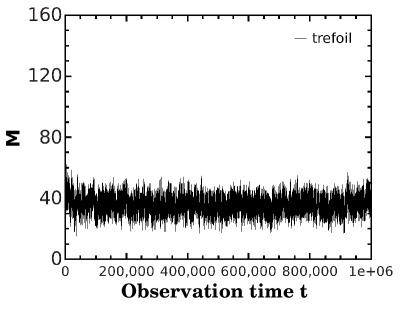
Figure 3: $M$ is the number of sites of the trefoil in which the direction of the chain is not changed.

Fig. 3, which is related to the latter method, shows that the system equilibrates after a few tens of thousands of pivot moves in the case of the trefoil ${\cal T}$. Similar considerations are valid for the other knots considered in this work. In total the system is subjected to one million of pivot moves before treating it with the WL algorithm in order to compute the energy $\langle E(\beta)\rangle$ and the heat capacity $C(T)$.

Now we briefly introduce the WL algorithm. This method is considered as a self-adjusting procedure for obtaining the density of states. In the present context the states are distinguished by the number $i$ of closest contacts between the polymer monomers, where $i$ takes positive integer values. Following a previous work pn , all initial values of the density of states are firstly set to be equal to one, i. e. $\Omega_{i}=1$ for all the states. Then the pivot method is used to visit the next trial state $i^{\prime}$. The energy of the trial state will be denoted by $\varepsilon m$, where $m$ is the number of the closest contacts of the monomers, while $\varepsilon$ is the interaction energy of each monomer pair. $\varepsilon>0$ and $\varepsilon<0$ correspond to repulsive and attractive case respectively. We assume in the following that $\varepsilon>0$. The probability of translating from the state $i$ to $i^{\prime}$ is

$$p(i-i^{\prime})=min[1,\dfrac{\Omega_{i}}{\Omega_{i^{\prime}}}]$$ (3)

Once an energy state is visited, the corresponding density of states of this state will be updated by multiplying a modification factor wanglaudau . After the $n-$th sweep, the modification factor $f_{i}$ is reduced according to the equation $f_{i+1}=\sqrt{f_{i}}$. The above process is repeated until the modification factor reaches the predefined limit $f_{final}=\exp(10^{-8})$ wanglaudau . Of course, at each step the preservation of the knot topology is checked with the method explained before. We show as an example the obtained densities of states for the unknot, the trefoil and the figure-eight of length $L=100$ in fig. 4.

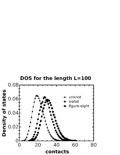
Figure 4: The density of states is obtained by WL algorithm. The results for the unknot (triangles), the trefoil (circles) and the figure-eight (rectangles) are represented.

The obtained distribution of density of energy states can now be used to calculate the canonical averages of the observables according to standard relations. As already mentioned, the observables studied in this paper are the internal energy of the canonical system and the heat capacity as a function of the temperature. The expression of the internal energy is given by:

$$\langle E(\beta)\rangle=\dfrac{\sum_{m}m\varepsilon e^{-\beta m\varepsilon}\Omega_{m}}{\sum_{m}e^{-\beta m\varepsilon}\Omega_{m}}$$ (4)

where $m$ is the number of the closest contacts of polymers and $\Omega(E)$ is the density of energy states computed by means of the WL algorithm. The formula of the heat capacity has been already provided in Eq. (1).

The computational method has been checked using the trivial knot $\cal U$ as a test. We could repeat the previous results of pnring in the case of chains with lengths equal to 12, 30 and 50.

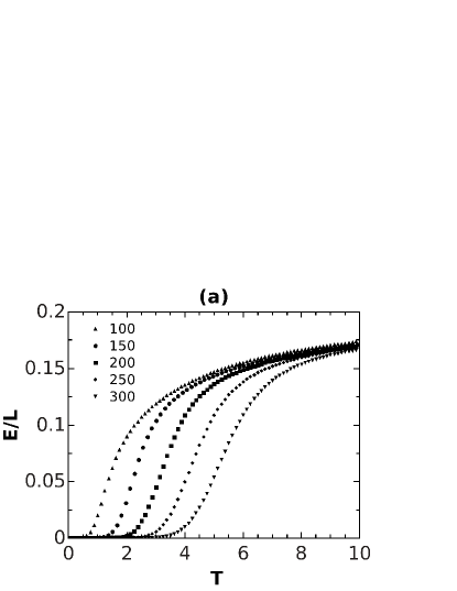
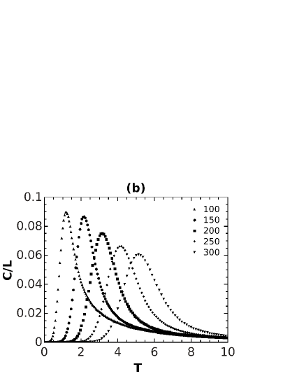
Figure 5: Specific energy and heat capacities for the unknot polymer as functions of the normalized temperature ${\mathbf{T}}=\frac{T}{\varepsilon}$. The polymer length can take the values $L=100\mbox{ (upper triangles)},150\mbox{ (circles)},200\mbox{ (rectangles)},250\mbox{ (diamonds)},300\mbox{ (down-triangles)}$, where $L$ denotes the number of steps. (a) Plot of the specific energy (in $\varepsilon$-units) of the unknot; (b) Plot of the specific heat capacity (in $\varepsilon$-units) of the unknot.

III results and discussion

In this section we study the thermal properties of the trefoil and figure-eight with lengths in the range of $100-300$ segments for the case $\varepsilon>0$. The used algorithm is quite fast. Depending on the length, the typical simulation times vary between 15 minutes to 1 hour on a dedicated pc. It can be applied to much more complicated knots. As an example, we have analysed here also the case of the $8_{1}$ knot.

The results concerning the trefoil and figure-eight are presented in fig. 6 and fig. 7 respectively. For comparison, fig. 5 represents the results for $\cal U$ with lengths ranging from $100$ to $300$. It is found that the growth of the specific energies $\langle E(\beta)\rangle/L$ in fig. 6(a) and fig. 7(a) is characterised by three regions both for the trefoil and the figure-eight. At very low temperatures the energy increase is practically zero. The reason is that the temperatures are too low to allow contacts between the monomers. When the energy of the system grows – let’s remember that we are working in energy units, so that we can talk about temperatures and energies interchangeably – the “first energy state” can be reached. This consists in the case in which at least two monomers are in contact. For instance, we expect that when the chain has length $L=100$, the first energy state occurs in figs. 6 and 7 at some “critical” temperature $T_{1}\sim 1$, while when $L=200$ this temperature should be given by $T_{1}\sim 2$. These values of $T_{1}$ slightly increase with increasing topological complexity. In general, this proportionality temperature/length is respected in figs. 6 and 7. After the first energy state is reached, the specific energy grows rapidly as a function of the temperature until saturation is reached after a given temperature $T_{2}$ and the energy increase becomes moderate. The division into three regions can be expected by looking at the Boltzmann factor $e^{-\beta m\varepsilon}$ appearing in the expression of the energy given in Eq. (4):

i) In the range $T<T_{1}$, the factor $e^{-\beta m\varepsilon}$ goes rapidly to $0$, because low temperatures cause few states to be occupied in this situation, so we get $\langle E\rangle\rightarrow 0$.

ii) When $T_{1}<T<T_{2}$, the factor $e^{-\beta m\varepsilon}$ changes sensitively depending on $\beta=T^{-1}$. In this regime more and more states of the given system are getting excited through heat absorption and $\langle E\rangle$ increases with the increase of the temperature $T$ as expected.

iii) Once $T>T_{2}$, $\langle E\rangle$ increases slower due to the fact that most states have been already occupied in the range $T_{1}<T<T_{2}$. Just few states are left that can be excited in this situation. One could notice that the factor $e^{-\beta m\varepsilon}$ in Eq. (4) increases slowly at high temperatures. When $T\rightarrow\infty$, we have $e^{-\beta m\varepsilon}\rightarrow 1$.

It can also be found that in fig. 6(b) and fig. 7(b), the heat capacity has a peak in the range of temperature $T_{1}<T<T_{2}$. The appearance of this peak together with the sigmoidal behavior of the specific energy points out at an ongoing two-state phase transition according to cooper . The presence of these pseudo-transitions related to the lattice geometry have been clarified in ref. wustlandau ; vogel .

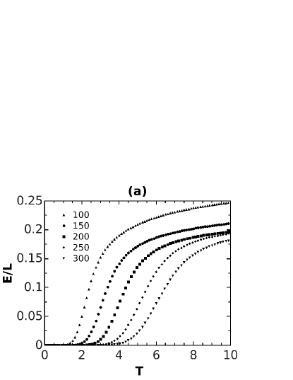
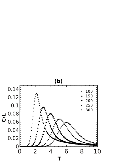
Figure 6: Specific energy and heat capacities for the trefoil as functions of the normalized temperature $\mathbf{T}=\frac{T}{\varepsilon}$. Separated plots are provided for trefoils with $L=100\mbox{ (upper triangles)},150\mbox{ (circles)},200\mbox{ (rectangles)},250\mbox{ (diamonds)},300\mbox{ (down-triangles)}$. (a) Plot of the specific energy (in $\varepsilon$-units) of the trefoil; (b) Plot of the specific heat capacity (in $\varepsilon$-units) of the trefoil.

We would also like to show that the heat capacity and energy are affected not only by the temperature, but also by the polymer length $L$ and its topological conformation. First of all, the specific energy of the chain decreases with increasing values of $L$. For instance, the quantity $\langle E(\beta)\rangle/L$ for $L=100$ is larger than that of longer chains as it is illustrated in fig. 6 and fig. 7. This is because longer polymers in the presence of short-range repulsive interactions prefer states which are diluted comparing with the short ones. Probably for this reason, in proteins knots are localized in regions with a very small number of residues dna . The total internal energy, instead, decreases with decreasing polymer lengths. This is due to the fact that longer polymers can accommodate a larger number of contacts. Let us note that the peak temperatures of the heat capacity are shifting with the length $L$. This is expected since we are computing the specific heat capacity. If we computed the total heat capacity of the system, these peaks would occur at the same temperature.

Concerning the topological effects, we observe that both the energy and the heat capacity increase with increasing knot complexity. This can be seen by comparing the plots for various knots of the same length in figs. 5, 6 and 7. On the other side, the topological effects are stronger when polymers are shorter. This is shown in Table 1 in which the energy differences for polymers with the same length but different topology are listed. In the table $d_{UT}$ is the difference between the unknot and the trefoil defined by $d_{\cal UT}\equiv\frac{\langle E_{\cal U}\rangle-\langle E_{\cal T}\rangle}{L}$, while $d_{\cal TF}$ denotes the difference between the trefoil and figure-eight. When the length ranges from $100$ to $300$, $d_{\cal UT}$ varies from $0.073$ to $0.015$ and $d_{\cal TF}$ from $0.032$ to $0.004$ at $T=10\varepsilon$. The heat capacity exhibits a similar behavior. It is thus pretty clear that the topological effects become less important when the length is increasing. This is similar to the so called ’size effect’ in nanomaterials yani . Topological properties will have a lesser influence in the case of diluted monomers. We expect that topological effects will disappear if the polymer is long enough.

Table 1: Energy differences between the unknot and the trefoil as well as those of the trefoil and figure-eight. All knots have the same length. The values of the energy difference are reported in the case of various lengths $L=100,200,300$. Here the temperature is $T=10\varepsilon$.

$L$	unknot	trefoil	figure-eight	$d_{\cal UT}$	$d_{\cal TF}$
100	0.174	0.247	0.279	0.073	0.032
200	0.170	0.197	0.210	0.027	0.013
300	0.167	0.182	0.186	0.015	0.004

To get a feeling of the size of the involved quantities, we can make the concrete example of the proteins which, as mentioned before, can be found in different topological conformations like the trefoil and the figure-eight. These proteins have a length of about 250 residues dna and their temperature is around $310K$ (since this is approximately the temperature of the human body). The parameter $\varepsilon$ for a protein is about $10K/mole$ ljwell . Based on those data, for one mole, we can roughly estimate the range of corresponding temperatures in our units, which is $T/\varepsilon=310K/\varepsilon=31$. This temperature is located in the region $T>T_{2}$.

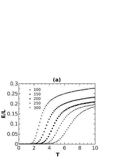
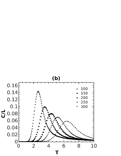
Figure 7: Specific energy and heat capacities for the figure-eight as functions of ${\mathbf{T}=\frac{T}{\varepsilon}}$. The lengths are $L=100\mbox{ (upper triangles)},150\mbox{ (circles)},200\mbox{ (rectangles)},250\mbox{ (diamonds)},300\mbox{ (down-triangles)}$ steps. (a) Plot of the specific energy (in $\varepsilon$-units) and (b) plot of the specific heat capacity (in $\varepsilon$-units) of the figure-eight knot.

Before concluding this section, we would like to stress that the used method for preserving the knot topology after a pivot move is very time efficient and can be applied to any knot configuration independently of its complexity. For example, in fig. 8 we provide the data for the specific energy and heat capacity in the case of the knot $8_{1}$. As it is possible to check, also for this knot the same conclusions drawn before for ${\cal K}={\cal T},{\cal F}$ are valid. In particular, the topological effects become less important with increasing polymer length and it is confirmed that both the energy and the heat capacity increase with increasing knot complexity.

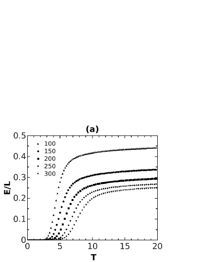
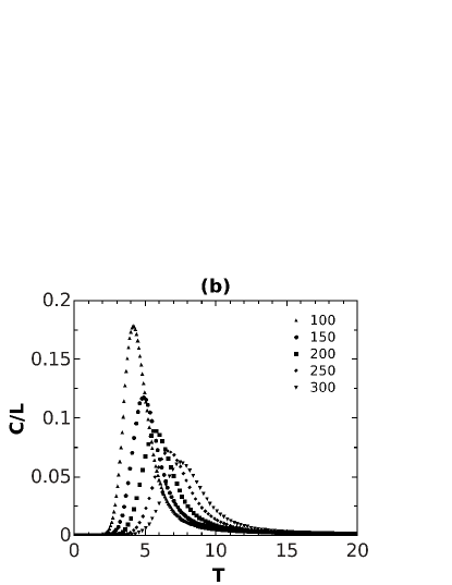
Figure 8: Specific energy and heat capacities for ${\cal K}=8_{1}$ as functions of $\mathbf{T}=\frac{T}{\varepsilon}$. The studied lengths are $L=100\mbox{ (upper triangles)},150\mbox{ (circles)},200\mbox{ (rectangles)},250\mbox{ (diamonds)}$ and $300\mbox{ (down-triangles)}$ steps. (a) Plot of the specific energy (in $\varepsilon$-units) and (b) specific heat capacity (in $\varepsilon$-units) of the $8_{1}$ knot.

IV Conclusions

We have studied the topological effects on the thermal properties of several knot configurations with the help of Monte Carlo simulations based on the Wang-Landau algorithm and the pivot method. The topology of the knots, that can change after a pivot move, has been preserved by explicitly checking if during the move some parts of the trajectory of the knot have crossed themselves at some points.

The specific energy and the heat capacity of the trefoil, the figure-eight and the $8_{1}$ knot have been calculated for various lengths ranging from $100$ to $300$. As a test of our methodology, these quantities have been derived also in the known case of the unknot. In particular, we have been able to reproduce the results of pnring . Our investigations show that the specific energy and heat capacity for a polymer knot whose monomers are subjected to short-range repulsive interactions are depending on the length and the topological conformation of the polymer knot. This could be expected because in the presence of repulsive interactions the polymer will prefer “diluted” conformations in which the monomer density is lower. We may thus suggest that the dilution of polymers in a good solvent should be effective in reducing the topological effects. Moreover, for the growth of the specific energy with respect to the temperature it is possible to distinguish three different regimes that have been explained in details in Section II. The zero energy regime appears at extremely low temperatures and it is characterised by the fact that the energy of the thermal fluctuations is below the threshold of the repulsive energy barrier, so that the monomers have not enough energy to get near. After this threshold has been passed, the number of contacts between the monomers starts to increase rapidly until at the end a saturation phenomenon occurs and the energy of the system increases only slowly with increasing temperatures. The plot of the specific heat capacity shows a pseudo-phase transition which is related to the lattice geometry, as explained in refs. wustlandau and vogel .

Our simulations can be generalised under several aspects. First of all, we limited ourselves to simple short range interactions, but there are no obstacles to extend our procedure to describe more realistic polymer systems. Moreover, we have limited ourselves to pivot moves involving a short number of segments. No difference between the case $N=4$ and $N=5$ have been detected, so that all displayed diagrams are related only to the case $N=5$. The independence of $N$ up to $N=10$ has been confirmed by preliminary calculations performed using another method to preserve the topology based on knot invariants. We hope to be able to report on these new developments very soon zhaoferrari .

- (1) A. Yu. Grosberg Phys.-Usp. 40, 12 (1997).
- (2) W. R. Taylor, Nature (London) 406, 916 (2000).
- (3) V. Katritch, J. Bednar, D. Michoud, R. G. Scharein, J. Dubochet, A. Stasiak, Nature 384, 142 (1996).
- (4) V. Katritch, W. K. Olson, P. Pieranski, J. Dubochet and A. Stasiak, Nature 388, 148 (1997).
- (5) M. A. Krasnow, A. Stasiak, S. J. Spengler, F. Dean, T. Koller and N. R. Cozzarelli, Nature 304, 559 (1983).
- (6) B. Laurie, V. Katritch, J. Dubochet and A. Stasiak, Biophys. Jour. 74, 2815 (1998).
- (7) J. I. Sułkowksa, P. Sułkowksa, P. Szymczak and M. Cieplak, Phys. Rev. Lett. 100, 058106 (2008).
- (8) Z. Liu, E. L. Zechiedrich, and H. S. Chan, Biophys. J. 90, 2344 (2006).
- (9) S. A. Wasserman and N. R. Cozzarelli, Science 232, 951 (1986).
- (10) D. W. Sumners, “Knot theory and DNA,” in New Scientific Applications of Geometry and Topology, edited by D. W. Sumners, Proceedings of Symposia in Applied Mathematics, Vol. 45, ͑American Mathematical Society, Providence, RI, 1992, 39.
- (11) A. V. Vologodski, ̵̆ A. V. Lukashin, M. D. Frank-Kamenetski ̵̆ and V. V. Anshelevich, Zh. Eksp. Teor. Fiz. 66, 2153 (1974); Sov. Phys. JETP 39, 1059 (1975); M. D. Frank-Kamenetskii, A. V. Lukashin and A. V. Vologodskii, Nature (London) 258, 398 (1975).
- (12) E. Orlandini, S. G. Whittington, Rev. Mod. Phys. 79, 611 (2007); C. Micheletti, D. Marenduzzo, and E. Orlandini, Phys. Reports 504, 1 (2011).
- (13) T. Vettorel, A. Yu. Grosberg and K. Kremer, Phys. Biol. 6, 025013 (2009).
- (14) P. Virnau, Y. Kantor and M. Kardar, J. Am. Chem. Soc. 127 (43), 15102 (2005).
- (15) P. Pierański, S. Przybył and A. Stasiak, EPJ E 6 (2), 123 (2001).
- (16) R. Metzler, A. Hanke, P. G. Dommersnes, Y. Kantor and M. Kardar, Phys. Rev. Lett. 88, 188101 (2002).
- (17) K. Koniaris and M. Muthukumar, Phys. Rev. Lett. 66, 2211 (1991).
- (18) R. Scharein et. al., J. Phys. A: Math. Gen. 43, 475006 (2009).
- (19) N. Madras, A. Orlistsky and L. A. Shepp, Journal of Statistical Physics 58, 159 (1990).
- (20) F. Wang and D. P. Laudau, Phys. Rev. Lett. 86, 2050 (2001).
- (21) C. Vree and S. G. Mayr, New Journal of Physics 12, 023001 (2010).
- (22) T. Kennedy, Jour. of Stat. Phys., 106 (3-4), 407-429 (2002).
- (23) P. N. Vorontsov-Velyaminov, N. A. Volkov and A. A. Yurchenko, J. Phys. A: Math. Gen. 37, 1573-1588 (2004).
- (24) N. A. Volkov, A. A. Yurchenko, A. P. Lyubartsev and P. N. Vorontsov-Velyaminov, Macromol. Theory Simul. 14, 491-504 (2005).
- (25) A. Cooper, Thermodynamics of protein folding and stability, in Protein: A Comprehensive Treatise, Vol. 2, A. G. Stamford (Ed.), JAI Press. Inc., 217 (1999).
- (26) T. Wüst and D. P. Landau, Phys. Rev. Lett. 102, 178101 (2009).
- (27) T. Vogel, M. Bachmann and W. Janke, Phys. Rev. E. 76, 061803 (2007).
- (28) Y.-N. Zhao, S.-X. Qu and Ke Xia, Jour. Appl. Phys. 110, 064312 (2011).
- (29) M. Schlosshauer and D. Baker, Protein Science 13, 1660 (2004).
- (30) Y. Zhao and F. Ferrari, work in progress.