Quantum Brayton cycle with coupled systems as working substance

Abstract

We explore the quantum version of Brayton cycle with a composite system as the working substance. The actual Brayton cycle consists of two adiabatic and two isobaric processes. Two pressures can be defined in our isobaric process, one corresponds to the external magnetic field (characterized by $F_{x}$) exerted on the system, while the other corresponds to the coupling constant between the subsystems (characterized by $F_{y}$). As a consequence, we can define two types of quantum Brayton cycle for the composite system. We find that the subsystem experiences a quantum Brayton cycle in one quantum Brayton cycle (characterized by $F_{x}$), whereas the subsystem’s cycle is of quantum Otto in another Brayton cycle (characterized by $F_{y}$). The efficiency for the composite system equals to that for the subsystem in both cases, but the work done by the total system are usually larger than the sum of work done by the two subsystems. The other interesting finding is that for the cycle characterized by $F_{y}$, the subsystem can be a refrigerator while the total system is a heat engine. The result in the paper can be generalized to a quantum Brayton cycle with a general coupled system as the working substance.

I Introduction

It is well know that there are four basic thermodynamical processes in classical thermodynamics: adiabatic process, isothermal process, isochoric process and isobaric process. These four processes correspond to entropy, temperature, volume and pressure being kept unchanged, respectively. The study on the quantum version for these processes can be dated back to the quantum adiabatic theorem Born ; Messiah , it brings the adiabat to quantum region and opens the door to quantum thermal dynamics. Recently, the isothermal and isochoric processes are generalized to quantum case Kieu2004PRL ; Kieu2006EPJD , and the quantum Carnot cycle and quantum Otto cycle are discussed in Quan2007PRE ; Quan2005PRE . With the definition of quantum isobaric processQuan2009PRE , almost all thermodynamical cycles, in particular Brayton cycle and Diesel cycle Callenbook ; Perrotbook , are extended from classical to quantum region.

The studies in the field of quantum thermodynamics Fialko2012PRL ; He2002PRE ; FeldmannPRE ; Wu2006JCP ; Lin2003PRE ; Li2007JPA are usually focused on whether it can surpass the classical limit on the efficiency and work extraction in a cycle Kieu2004PRL ; Kieu2006EPJD ; Scully2003Science , and how to better the work extraction in a cycle WangPRE . For example, it is reported that one can extract work from a single heat bath via vanishing quantum coherence Scully2003Science and the efficiency of a quantum heat engine can be higher than the classical one due to the effects of squeezing heat bath Huangsubmit . These studies can better our understanding of the fundamental concept in thermodynamics and quantum mechanics, and bring new insights into basic problems in quantum mechanics and thermodynamics Quan2006 ; ScullyPRL .

Coupled quantum system as working substance becomes an active topic recentlyZhang2007PRA ; Wang2009PRE ; Zhang2008EPJD ; Thomas2011PRE . The reason is twofold. First, the entanglement is one of the features that distinguish quantum and classical worlds, the effects of quantum entanglement on the basic thermodynamical quantities are then attractive Zhang2007PRA ; Wang2009PRE ; Zhang2008EPJD . Second, for a cycle with coupled quantum system as the working substance, the effects of coupling on the cycle is an interesting problem Thomas2011PRE , besides, the thermodynamical relations for the coupled system and its subsystems are also interesting. Indeed, previous study shown that in a Otto cycle with coupled quantum system as its working substance, the total coupled system may absorb heat from the hot bath and releases heat to the cold bath, while the subsystem absorbs heat at the cold bath and releases heat at the hot bath with a net work doneThomas2011PRE .

Motivated by these works, here we study the effects of coupling on the quantum isobaric process and the quantum Brayton cycle. Two coupled spins are considered as the working substance, the thermodynamical relations for the total system and its subsystem are studied and several interesting results are observed. These observations hold true for a general coupled system as the working substance. This paper is organized as follows. In Sec.II, we first give a brief introduction to the pressure in quantum processes and quantum Brayton cycle, then we examine the Brayton cycle with a single spin in external magnetic field as the working substance. In Sec.III, the detailed analysis for the quantum isobaric process and Brayton cycle with coupled system as working substance is presented. Discussions on the generality of our results and conclusions are given in Sec.IV.

II Quantum isobaric process and quantum Brayton cycle for spin-$1/2$ system in an external magnetic field

In this paper, we use the definition of quantum pressure given in Ref.Quan2009PRE as

$$F=-\sum_{n}p_{n}\frac{dE_{n}}{dL},$$ (1)

where $L$ is the generalized coordinate of the system. This definition is deduced from the quantum version of the first law of thermodynamics $dU=\sum_{n}E_{n}dp_{n}+\sum_{n}p_{n}dE_{n}\equiv\mkern 3.0mu\mathchar 22\relax\mkern-12.0mudQ+\mkern 3.0mu\mathchar 22\relax\mkern-12.0mudW=TdS+\sum_{n}Y_{n}dy_{n}$ and an analogy of classical relation between the generalized force and the generalized coordinate as $Y_{n}=-\frac{\mkern 3.0mu\mathchar 22\relax\mkern-12.0mudW}{dy_{n}}$, where $T$ and $S$ refer to temperature and thermodynamical entropy, respectively, $Y_{n}$ is the generalized force and $y_{n}$ is its conjugated generalized coordinate ($dy_{n}$ can be seen as the generalized displacement). We should mention that for a one dimensional system, the generalized force is the same as pressure. We first consider a spin-$1/2$ system in an external magnetic field as the working substance. The Hamiltonian of the working substance can be written as $H=\frac{1}{2}B\sigma^{z}$. For the working substance at thermal equilibrium, choosing the inverse of the magnetic field as the generalized coordinate $L=1/B$, we can calculate the generalized force Eq.(1) as

$$F=-\frac{\tanh(\frac{\beta}{2L})}{2L^{2}},$$ (2)

where $\beta=1/kT$, $T$ is the temperature of the system and $k$ is the Boltzmann constant. Then a quantum isobaric process can be defined as a process with constant force $F$, which can be realized by controlling carefully the temperature $T$ (or $\beta$) and the magnetic field $B$ (or $L$) by Eq.(2). We should note that the expression for the pressure varies from system to system, because we do not have a unique equation of spectrum for quantum system. This was confirmed in Sec.III.

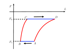
Figure 1: (Color online) Force-displacement $F-L$ diagram of a quantum Brayton cycle, we plot this figure by using the data from the spin-$\frac{1}{2}$ as the working substance.

A quantum Brayton cycle is a generalization of the classical Brayton cycle Callenbook ; Perrotbook to quantum case, which consists of two quantum adiabatic processes and two quantum isobaric processes (see Fig.1). Starting from point $A$, the four stages of a cycle can be depicted as follows: Stage 1: $A\rightarrow B$ is an isobaric process, in which the generalized force $F_{1}$ keeps. The system absorbs heat from the environment and some work is done on the system. In order to ensure that the heat is absorbed from the environment, we should have $L_{B}<L_{A}$. Stage 2: $B\rightarrow C$ is an adiabatic process, where only some work is done by the system. Stage 3: $C\rightarrow D$ is almost an inverse process of stage 1 that the generalized force is replaced by $F_{0}$. Stage 4: $D\rightarrow A$ is another adiabatic process. In the isobaric process the generalized force keeps constant while in the quantum adiabatic process the entropy of the system is unchanged. The entropy of the system is

$$S=k[\ln(2\cosh\frac{\beta}{2L})-\frac{\beta}{2L}\tanh\frac{\beta}{2L}].$$ (3)

It is easy to find that in the quantum adiabatic process we have $TL{=}$const (or $\beta/L{=}$const). Based on this fact, we can get a further equation in quantum adiabatic process from Eq.(2) as

$$FL^{2}=\text{const}.$$ (4)

The internal energy of the system is

$$U=-\frac{1}{2L}{\tanh{\frac{\beta}{2L}}}.$$ (5)

Comparing it with Eq.(2) we find $FL=U$. These two relations together yield the basic thermodynamics quantities such as heat transfer, net work done by the system and efficiency, as follows,

$$Q_{AB} = \int_{L_{A}}^{L_{B}}\sum_{n}E_{n}dp_{n}$$

$$= \left.\sum_{n}p_{n}E_{n}\right|_{L_{A}}^{L_{B}}-\int_{L_{A}}^{L_{B}}\sum_{n}p_{n}\frac{dE_{n}}{dL}dL$$

$$= U(L_{B})-U(L_{A})+\int_{L_{A}}^{L_{B}}F_{1}dL=2F_{1}(L_{B}-L_{A}),$$

$$Q_{CD} = 2F_{0}(L_{C}-L_{D}),$$

$$W = Q_{AB}-Q_{CD},$$

$$\eta = 1-\frac{Q_{CD}}{Q_{AB}}=1-\sqrt{\frac{F_{0}}{F_{1}}}.$$

We can see from this equation that the system absorbs heat in the process $A\rightarrow B$ and releases heat in the process $C\rightarrow D$. The efficiency is consistent to the classical result $\eta=1-(\frac{F_{0}}{F_{1}})^{1-1/\gamma}$, where $\gamma$ is the adiabatic exponent. In this model, we have shown that in the quantum adiabatic process $TL{=}$const. Comparing with $TL^{\gamma-1}{=}$const for the classical adiabatic process, the adiabatic exponent is $\gamma=2$. These result can be found in the coupled system as the working substance, as we will show below.

III Quantum isobaric process and quantum Brayton cycle with two coupled spin-$1/2$s as the working substance

The main purpose of this paper is to study the quantum isobaric process and quantum Brayton cycle for a coupled system as the working substance and to consider the effect of coupling on the cycle. The Hamiltonian for the working substance under consideration is

$$H=\frac{B}{2}(\sigma^{z}_{1}+\sigma^{z}_{2})+J(\sigma^{+}_{1}\sigma^{-}_{2}+\sigma^{-}_{1}\sigma^{+}_{2}),$$ (6)

where $J$ is the coupling constant between the spins. $J>0$ and $J<0$ correspond to the antiferromagnetic and the ferromagnetic case, respectively. Here we only consider the antiferromagnetic case, i.e., $J>0$. The four eigenvalues and corresponding eigenstates can be easily obtained as

$$E_{1}=-B,~{}~{}~{}|\psi_{1}\rangle=|00\rangle,$$

$$E_{2}=-J,~{}~{}~{}~{}|\psi_{2}\rangle=\frac{1}{\sqrt{2}}(|01\rangle-|10\rangle),$$

$$E_{3}=J,~{}~{}~{}~{}~{}~{}|\psi_{3}\rangle=\frac{1}{\sqrt{2}}(|01\rangle+|10\rangle),$$

$$E_{4}=B,~{}~{}~{}~{}~{}|\psi_{4}\rangle=|11\rangle.$$ (7)

There are two independent parameters in the Hamiltonian, and hence we need two generalized coordinates to describe the system. Choosing $X=1/B$ and $Y=1/J$ as the generalized coordinates, we can define two generalized forces (or pressures) corresponding to $X$ and $Y$, respectively, as

$$F_{x}=-\frac{\sinh\frac{\beta}{X}}{X^{2}(\cosh\frac{\beta}{X}+\cosh\frac{\beta}{Y})},$$ (8)

$$F_{y}=-\frac{\sinh\frac{\beta}{Y}}{Y^{2}(\cosh\frac{\beta}{X}+\cosh\frac{\beta}{Y})}.$$ (9)

The quantum isobaric process for this system means either $F_{x}$ or $F_{y}$ is fixed. As a result, we will discuss these two different cases separately. The expression for the entropy is complicated, hence we do not want to write it here. Noting that the entropy in a quantum adiabatic process is unchanged, we have

$$XT=\text{const},~{}~{}YT=\text{const},~{}~{}\frac{X}{Y}=\text{const}.$$ (10)

This means that all the spacings of energy-level for the working substance change by the same ratio, this together with another restriction we adopted in Sec.II, i.e., this ratio equals to the ratio of the temperature of the substance before the adiabatic process to that after the adiabatic process, guarantee the reversible cycle. The discussion in this paper focuses exactly on this reversible quantum Brayton cycle. The internal energy of the system can be written as

$$U=-\frac{Y\sinh\frac{\beta}{X}+X\sinh\frac{\beta}{Y}}{XY(\cosh\frac{\beta}{X}+\cosh\frac{\beta}{Y})}=F_{x}X+F_{y}Y,$$ (11)

which will be used in the following discussions. We should also note that in the following discussion, we consider the relation between the total system and subsystem in the cycle. We will denote the symbol $F_{\text{loc}}$ or the concept of local force to the force corresponding to the local magnetic field $B$ for one of the subsystems.

III.1 Fixed $F_{x}$

We first consider the relation between the composite system and its subsystems in quantum isobaric process when the generalized force $F_{x}$ is fixed. In this process, the generalized coordinate and the temperature are controlled according to Eq.(8) such that $F_{x}$ is a constant with the generalized coordinate $Y$ as another constant. We will prove that both of the subsystems undergo a quantum isobaric process when the generalized force $F_{x}$ is fixed and the generalized force for the subsystems equals to $\frac{1}{2}F_{x}$. As a consequence, the cycle for the subsystem is also a quantum Brayton cycle.

Proof: the state of the composite system is in a thermal equilibrium state which can be easily calculated as

$$\rho(T){=}\sum_{n}p_{n}|\psi_{n}\rangle\langle\psi_{n}|{=}\left(\begin{array}[]{cccc}p_{4}&0&0&0\\ 0&\frac{1}{2}(p_{2}{+}p_{3})&\frac{1}{2}(p_{3}{-}p_{2})&0\\ 0&\frac{1}{2}(p_{3}{-}p_{2})&\frac{1}{2}(p_{2}{+}p_{3})&0\\ 0&0&0&p_{1}\\ \end{array}\right),$$ (16)

where $p_{n}=\frac{1}{\mathcal{Z}}\exp(-\frac{E_{n}}{kT})$, and $T$ is the temperature of the composite system. ${\mathcal{Z}}=\sum_{n}\exp(-\frac{E_{n}}{kT})$ is the partition function of the system. For the reduced system, we can get the reduced state by tracing out its partner as

$$\rho_{A}=\rho_{B}=\left(\begin{array}[]{cc}p_{4}+\frac{1}{2}(p_{2}+p_{3})&0\\ 0&p_{1}+\frac{1}{2}(p_{2}+p_{3})\\ \end{array}\right).$$ (19)

This state can be seen as an equilibrium state with a local effective temperature $\beta_{\text{loc}}$ (or $T_{\text{loc}}$) as

$$\beta_{\text{loc}}=X\ln\frac{p_{1}+\frac{1}{2}(p_{2}+p_{3})}{p_{4}+\frac{1}{2}(p_{2}+p_{3})}.$$ (20)

According to the definition of generalized force for a single spin in Sec.II, we arrive at

$$F_{\text{loc}}=-\frac{1}{2X^{2}}\tanh(\frac{\beta_{\text{loc}}}{2X}).$$ (21)

By virtue of the formula $\tanh(\frac{1}{2}\ln x)=\frac{x-1}{x+1}$ and the definition for $F_{x}$ (Eq.(8)) we have

$$F_{\text{loc}}=-\frac{\sinh\frac{\beta}{X}}{2X^{2}(\cosh\frac{\beta}{X}+\cosh\frac{\beta}{Y})}=\frac{1}{2}F_{x}.$$ (22)

This result shows that if the composite system keeps the generalized force $F_{x}$ unchanged, the generalized force for subsystems is also a constant and it equals to $\frac{1}{2}F_{x}$.

In the following, we consider the quantum Brayton cycle based on the coupled system when $F_{x}$ is fixed. Similar to the case for a single spin, we decrease $X$ in stage 1 and adjust the temperature $T$, so that $F_{x1}$ keeps unchanged. Moreover, the parameters $Y_{1}$, which is the inverse of the coupling constant, is also unchanged in this stage. In the adiabatic process, Eq.(10) should be satisfied so that the cycle is reversible. After this stage, the parameter becomes $Y_{0}$ and in stage 3 it keeps as a constant. The force in stage 3 is $F_{x0}$. The heat absorbed by the system during the stage 1 is

$$Q_{AB}{=}\int_{X_{A}}^{X_{B}}\sum_{n}E_{n}dp_{n}{=}U(X_{B}){-}U(X_{A}){+}\int_{X_{A}}^{X_{B}}F_{x1}dX$$

$$~{}~{}~{}~{}=2F_{x1}(X_{B}-X_{A})+(F_{yB}-F_{yA})Y_{1}.$$ (23)

We can see from the above expression that $Q_{AB}$ depends not only on the force $F_{x}$ but also on the force $F_{y}$ and the coupling constant. This means that the interaction between the two spins has a strong effect on the cycle. Similarly, we can calculate the heat released to environment in stage 3 as

$$Q_{CD}=2F_{x0}(X_{C}-X_{D})+(F_{yC}-F_{yD})Y_{0}.$$ (24)

Hence the efficiency of the cycle can be expressed as

$$\eta_{x}=1-\frac{Q_{CD}}{Q_{AB}}=1-\sqrt{\frac{F_{x0}}{F_{x1}}}.$$ (25)

The detailed derivation about the above equation is given in appendix A. This result is the same to the single spin case. After the same procedure as given in Sec.II, we can get the efficiency for the subsystem as

$$\eta_{\text{loc}}=1-\sqrt{\frac{F_{\text{loc}0}}{F_{\text{loc}1}}}=1-\sqrt{\frac{F_{x0}}{F_{x1}}},$$ (26)

This equation shows that the efficiency for the composite system as working substance is the same to the one for its subsystem. The net work done by the composite system is

$$W=[2F_{x1}(X_{B}-X_{A})-2F_{x0}(X_{C}-X_{D})]$$

$$~{}~{}~{}~{}~{}~{}~{}~{}~{}~{}~{}~{}+[(F_{yB}-F_{yA})Y_{1}-(F_{yC}-F_{yD})Y_{0}].$$ (27)

The first $[\cdot]$ on the right hand side can be seen as the sum of the work done by the two subsystem while the second $[\cdot]$ comes from the effects of interaction between the two subsystems. Due to the positivity of this term, we have $W>2W_{\text{loc}}$, i.e., the total work performed is larger than the sum of work obtained from the two spins locally. Numerical examples for this result is shown in Fig.2. From the figure we claim that the coupling can increase the net work done by the system during a cycle although the efficiency is not improved. When $J=0$, $W/W_{\text{loc}}=2$ in all cases as expected. Another point to be explained is that in Fig.2, some lines are crossed. The reason is that when the absolute value of $F_{x1}$ is larger, the possible region for the coupling constant is smaller.

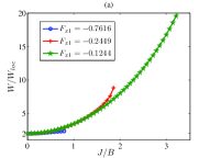
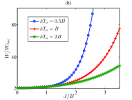
Figure 2: (Color online) Efficiency and net work done by the coupled system as a function of $J/B$ at point $A$ when (a) initial pressure $F_{x1}$ (b) initial temperature $kT_{a}$ is fixed. Other parameters in the figure are $F_{x0}=\frac{1}{4}F_{x1}$, $\frac{X_{A}}{X_{B}}=\frac{X_{D}}{X_{C}}=3$.

III.2 Fixed $F_{y}$

Similar to the discussion given above, an isobaric process that $F_{y}$ is fixed means one should carefully control the coordinate $Y$ and temperature $T$ such that $F_{y}$ is a constant with $X$ as another constant. It can be easily verified that during this process, the pressure for the subsystem is not fixed, i.e., the process for the subsystem is not a quantum isobaric process. However, when we control the coordinate $Y$ for the composite system, the local Hamiltonian for the subsystem does not vary and the energy levels for the subsystem keep as constants. As a result, the subsystems undergo quantum isochoric process when $F_{y}$ is fixed, and a quantum Brayton cycle based on $F_{y}$ for the composite system results in a quantum Otto cycle for the subsystem.

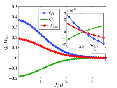
Figure 3: (Color online) The local heat exchange $Q_{1}$ and $Q_{2}$ and the local work $W_{\text{loc}}$ (in units of $B$) as a function of $J/B$. Here the initial temperature $kT_{a}=0.5B$. Other parameters are $F_{y0}=\frac{1}{4}F_{y1}$, $\frac{Y_{A}}{Y_{B}}=\frac{Y_{D}}{Y_{C}}=3$.

After some calculations which are similar to Sec.III.1, we obtain the efficiency of the cycle for the composite system as

$$\eta_{y}=1-\sqrt{\frac{F_{y0}}{F_{y1}}}.$$ (28)

The efficiency for the subsystem can be obtained according to the efficiency of quantum Otto cycle as

$$\eta_{\text{loc}}=1-\frac{X_{1}}{X_{0}}=1-\sqrt{\frac{F_{y0}}{F_{y1}}}.$$ (29)

This result tells us that the efficiency for the composite system during a quantum Brayton cycle with fixed $F_{y}$ equals to the one for the subsystem during a quantum Otto cycle, conditioned on that the subsystem is a Otto heat engine. We should note that when initial temperature is small enough and the coupling constant is large enough, the work done by the subsystem can be negative. In this case, the subsystem is a refrigerator while the total system is a heat engine. Numerical examples are given in Fig.3. In this figure we show the heat exchange $Q_{1}$ in stage 1 and $Q_{2}$ in stage 3 for the subsystem. Here $Q_{i}>0$ and $Q_{i}<0$ ($i=1,2$) correspond to absorption and release of heat, $W_{\text{loc}}$ is the local work. From the figure we see that when initial $J/B$ at point $A$ is larger than a certain value, $Q_{1}<0$, $Q_{2}>0$ and $W_{\text{loc}}<0$. This indicates that the subsystem is a refrigerator, it releases heat when the composite system absorbs heat in stage 1 and goes opposite in stage 3. The condition for such a phenomenon is that $p_{e}^{B}<p_{e}^{A}$, where $p_{e}^{i}=p_{4}^{i}+\frac{1}{2}(p_{2}^{i}+p_{3}^{i})$ is the probability for the subsystem on its excited state at point $i(i=A,B)$. The feature comes from the strange property for the eigenstate $|\psi_{3}\rangle$ of the system. In the strong coupling regime, the ground state of the system is $|\psi_{3}\rangle$. However, the reduced state for this state is $\rho_{A(B)}=\frac{1}{2}I_{2}$, which can be seen as an equilibrium state at a local effective temperature $T_{\text{loc}}=\infty$. Here $I_{2}$ is a $2\times 2$ unit matrix. Hence in stage 1, when the global temperature is low enough and the coupling constant is large enough, the global temperature increases while the local temperature decreases. Hence the subsystem releases heat in stage 1 and inversely in stage 3. As a result the local cycle is a refrigeration cycle.

IV Discussions and Conclusions

Before concluding, we briefly discuss the generality of our results. The conclusion holds true for two spin-$\frac{1}{2}$s with general couplings described by the following Hamiltonian, $H=\frac{J}{2}[(1+\gamma)\sigma^{x}_{1}\sigma^{x}_{2}+(1-\gamma)\sigma^{y}_{1}\sigma^{y}_{2}]+J\Delta\sigma^{z}_{1}\sigma^{z}_{2}+\frac{B}{2}(\sigma^{z}_{1}+\sigma^{z}_{2})$, where $\gamma$ and $\Delta$ are anisotropy parameters. The four eigenvalues and corresponding eigenstates for this Hamiltonian are $E_{1}=J\Delta-\sqrt{B^{2}+J^{2}\gamma^{2}},|\psi_{1}\rangle=\cos\theta|11\rangle-\sin\theta|00\rangle,E_{2}=-J(1+\Delta),|\psi_{2}\rangle=\frac{1}{\sqrt{2}}(|01\rangle-|10\rangle),E_{3}=J(1-\Delta),|\psi_{3}\rangle=\frac{1}{\sqrt{2}}(|01\rangle+|10\rangle),E_{4}=J\Delta+\sqrt{B^{2}+J^{2}\gamma^{2}},|\psi_{4}\rangle=\sin\theta|11\rangle+\cos\theta|00\rangle$, where $\tan\theta=\frac{B+\sqrt{B^{2}+J^{2}\gamma^{2}}}{J\gamma}$. If $\gamma=\Delta=0$, the model returns to the Hamiltonian given in Eq.(6). For the system with general couplings, we still choose $X=\frac{1}{B}$ and $Y=\frac{1}{J}$ as the generalized coordinates and define the generalized forces $F_{x}$ and $F_{y}$ similar to our earlier discussions in this paper. For the quantum Brayton cycle characterized by the generalized force $F_{x}$, we can prove in the same manner that the cycle for the subsystem is also a quantum Brayton cycle and the efficiencies for the subsystem and total system are equal. However, for the quantum Brayton cycle with fixed $F_{y}$, the cycle for the subsystem is a Otto cycle. The situation that the total system is a heat engine while the subsystem operators as a refrigerator can happen when $p_{e}^{B}<p_{e}^{A}$, where $p_{e}$ is the population of the excited state at point $i(i=A,B)$. This is similar to the discussion in the last section. For the two spins with generalized couplings, it is involved to give an analytical result, the following analysis would help understanding the prediction in such systems.

We now focus on the result that the total system behaves like a heat engine but the subsystem behaves like a refrigerator. The essence of this result is that in one of the four stages of the cycle the total system absorbs heat while the subsystem releases heat. A similar result was observed in Ref.Thomas2011PRE , where a coupled Otto cycles was considered. There are four basic thermodynamical processes in quantum thermodynamics. It is obviously that this feature can not happen in a quantum adiabatic process. Based on our results and the results in Ref.Thomas2011PRE , we know that it can happen in quantum isobaric process and quantum isochoric process. The only process that has not been discussed to date is the quantum isothermal process for coupled systems in which the situation is more complicated because the process for the subsystem might be not any one of the four basic thermodynamical processes. Hence the heat transfer for the subsystem is difficult to handle. Here we only give an extreme example by considering the system given in Eq.(6) undergoes a quantum isothermal process with absolute zero temperature $T=0$. In this process, the magnetic field $B$ decreases slowly so that the system is always in the ground state. Initially, $B>J$, the ground state is $|\psi_{1}\rangle=|00\rangle$. As a result, the subsystem are also in the ground state (effective temperature $T_{\text{eff}}=0$). After some time, when $B<J$, $|\psi_{2}\rangle$ becomes the ground state of the total system. Hence, the state for the subsystem becomes $\rho_{A}=\rho_{B}=\frac{1}{2}I_{2}$, a state with the effective temperature $T_{\text{eff}}=\infty$. In this process, the generalized coordinate, generalized force, effective temperature and entropy for the subsystem are all changed. As a result, none of the four basic thermodynamical processes match the behavior of the subsystem. The case in which the heat transfer is different between the total system and subsystem may also happen under certain condition in an isothermal process. This can be understood as follows. From the energy spectrum of the composite system given in Eq.(7) we know that the entropy of the system $S=S(B,J)=-k\sum_{n}p_{n}\ln p_{n}$ is symmetric about $B$ and $J$, i.e., this expression does not change when we exchange the two variables $B$ and $J$. Then we take a total differential for $S$ as $dS=\left(\frac{\partial S}{\partial B}\right)dB+\left(\frac{\partial S}{\partial J}\right)dJ$. Initially we set $B=J$. Due to the symmetry of the entropy, we have $\left(\frac{\partial S}{\partial B}\right)=\left(\frac{\partial S}{\partial J}\right)<0$. Now we consider two processes as follows: (i) $B\rightarrow B+dB$; (ii) $J\rightarrow J+dJ$. Here $dB$ and $dJ$ denote infinitesimal increment for magnetic field and coupling constant, respectively. We assume $dB>0$ and $dJ>0$. It can be easily proved that $dS<0$ for these two processes. Hence in these two isothermal processes, ${\mathchar 22\relax\mkern-11.0mud}Q=TdS<0$, i.e., the total system releases heat to the heat bath in both cases. However, the heat transfer are different for the subsystem in these two processes. This can be seen obviously in the limit $\beta\rightarrow\infty$ (or $T\rightarrow 0$, i.e. the low temperature behavior). With this limitation and initial condition $B=J$, we can obtain the state of the subsystem as $\rho_{Ai}=\rho_{Bi}=\frac{1}{4}|\uparrow\rangle\langle\uparrow|+\frac{3}{4}|\downarrow\rangle\langle\downarrow|$ (In fact, when $T\neq 0$, this is not the exact state for the subsystem, however when the temperature is low enough, the probability of the subsystem in this state is higher that 0.99, hence we analyze the heat transfer according to this approximate state). Then we consider the following two processes separately. (i) $B\rightarrow B+dB$. In this case, $|\psi_{1}\rangle$ is the ground state of the total system. As a result, $\rho_{Af}=\rho_{Bf}=|\downarrow\rangle\langle\downarrow|$. During this process, the internal energy of the subsystem decreases. The work done in this process is infinitesimal. Hence the subsystem releases heat. (ii) $J\rightarrow J+dJ$. $|\psi_{2}\rangle$ becomes the ground state of the total system, then $\rho_{Af}=\rho_{Bf}=\frac{1}{2}I_{2}$. Hence the subsystem absorbs heat. We can see in the case (ii) that the heat transfer is different between the total system and the subsystem in a quantum isothermal process. Based on the discussion above, we conclude that the thermodynamical cycle which consists of the quantum adiabatic process and one or two of other three processes (for example, Carnot cycle and Diesel cycle) can have the similar property that the heat flow of the subsystem and total system are in the opposite directions, namely, the total system absorbs heat while the subsystem releases heat.

In summary, with coupled spins as working substance, the quantum isobaric process and the quantum Brayton cycle have been studied in this paper. The concept of force or pressure in quantum system is deduced from the quantum version of the first law of thermodynamics and an analogy of classical relation between generalized force and generalized coordinate Quan2009PRE . The quantum Brayton cycle consists of two quantum adiabatic processes and two quantum isobaric processes. There are two generalized coordinates in our system, i.e., the local external magnetic field and the coupling constant, therefore we can define two pressures respectively and construct two types of quantum Brayton cycle. We find that in quantum Brayton cycle based on the pressure corresponding to the external field, the subsystem undergo a quantum Brayton cycle with pressure half of the total system, while in the cycle based on the force conjugated to the coupling strength, the subsystem experiences a quantum Otto cycle. The efficiency for the coupled system in the two cycles are equal to that for the subsystem, which is the same as the classical result, but the net work done by the total system are usually more than the sum of works done by the subsystems. Moreover, when the initial temperature and initial coupling strength are chosen properly, an interesting phenomenon can be observed in the Brayton cycle based on the force corresponding to coupling constant, i.e., the total system performed as a heat engine while the subsystems serve as a refrigerator. The essence for this interesting result is that the heat flows to different directions in the subsystems and in the whole system. This can happen in quantum isochoric process and quantum isothermal process, which is a reminiscence of the non-locality of quantum system in thermodynamics.

This work is supported by NSF of China under Grant Nos. 11105064, 10905007, and 11175032.

Appendix A The derivation of $\eta$ for the coupled system when $F_{x}$ is fixed.

First, from expression of $F_{x}$ in Eq.(8) and the condition for adiabatic process in Eq.(10), we have

$$F_{x}X^{2}=\text{const}$$ (30)

As a result, one can construct the relation during the two adiabatic processes as

$$\frac{F_{x0}}{F_{x1}}=\frac{X_{B}^{2}}{X_{C}^{2}}=\frac{X_{A}^{2}}{X_{D}^{2}}.$$ (31)

In the similar manner, for the force $F_{y}$ we obtain

$$F_{y}Y^{2}=\text{const}$$ (32)

and

$$\frac{Y_{1}^{2}}{Y_{0}^{2}}=\frac{F_{yC}}{F_{yB}}=\frac{F_{yD}}{F_{yA}}.$$ (33)

Moreover, based on $\frac{X}{Y}=\text{const}$ in the adiabatic process, we have

$$\frac{Y_{1}}{Y_{0}}=\frac{X_{A}}{X_{D}}=\frac{X_{B}}{X_{C}}$$ (34)

Combining Eqs.(31), (33) and (34), we obtain a complete ratio relation for the whole cycle as

$$\frac{Y_{1}^{2}}{Y_{0}^{2}}=\frac{X_{A}^{2}}{X_{D}^{2}}=\frac{X_{B}^{2}}{X_{C}^{2}}=\frac{F_{x0}}{F_{x1}}=\frac{F_{yC}}{F_{yB}}=\frac{F_{yD}}{F_{yA}}.$$ (35)

Using this equation we can obtain Eq.(25). In a similar way Eq.(28) can be obtained.

References

- (1) M. Born and V. Fork. Z. Phys. 51, 165 (1928).
- (2) A. Messiah, Quantum Mechanics (Dover, New York, 1999).
- (3) T. D. Kieu, Phys. Rev. Lett. 93, 140403(2004).
- (4) T. D. Kieu, Eur. Phys. J. D 39, 115 (2006); quan-ph/0311157.
- (5) H. T. Quan. P. Zhang, and C. P. Sun, Phys. Rev. E 72, 056110(2005).
- (6) H. T. Quan, Y. X. Liu, C. P. Sun, and F. Nori, Phys. Rev. E 76, 031105(2007).
- (7) H. T. Quan, Phys. Rev. E 79, 041129(2009).
- (8) H. B. Callen, Thermodynamics and an Introduction to Themostatistics, 2nd ed. (Wiley, New York, 1985); C. Kittle and H. Kroemer, Thermal Physics, 2nd ed. (Freeman, San Francisco, 1980).
- (9) P. Perrot, A to Z of Thermodynamics (Oxford University Press, Oxford, 1998).
- (10) O. Fialko and D. W. Hallwood, Phys. Rev. Lett. 108, 085303(2012).
- (11) J. Z. He, J. C. Chen, and B. Hua, Phys. Rev. E 65, 036145(2002).
- (12) T. Feldmann and R. Kosloff, Phys. Rev. E 61, 4774(2000); Phys. Rev. E 68, 016101(2003); Phys. Rev. E 70, 046110(2004).
- (13) F. Wu, L. G. Chen, S. Wu, F. R. Sun, C. Wu, J. Chem. Phys. 124, 214702(2006).
- (14) B. H. Lin and J. C. Chen, Phys. Rev. E 67, 046105(2003).
- (15) S. Li, H. Wang, Y. D. Sun, and X. X. Yi, J. Phys. A 40, 8655 (2007).
- (16) M. O. Scully, M. S. Zubairy, G. S. Agarwal, and H. Walther, Science 299, 862(2003).
- (17) J. H. Wang, H. Z. He, and X. He, Phys. Rev. E 84, 041127(2011); J. H. Wang, H. Z. He, and Z. Q. Wu, Phys. Rev. E 85, 031145(2012); J. H. Wang, Z. Q. Wu, and J. Z. He, Phys. Rev. E 85, 041148(2012); J. H. Wang and J. Z. He, J. Appl. Phys. 111, 043505(2012).
- (18) X. L. Huang, Tao Wang, and X. X. Yi, Phys. Rev. E 86, 051105(2012).
- (19) M. O. Scully, Phys. Rev. Lett. 87, 220601(2001); Phys. Rev. Lett. 88, 050602(2002).
- (20) H. T. Quan, Y. D. Wang, Y. X. Liu, C. P. Sun, and F. Nori, Phys. Rev. Lett. 97, 180402(2006); H. T. Quan. P. Zhang, and C. P. Sun, Phys. Rev. E 73, 036122(2006).
- (21) T. Zhang, W. T. Liu, P. X. Chen, and C. Z. Li, Phys. Rev. A 75, 062102(2007).
- (22) H. Wang, S. Q. Liu, and J. Z. He, Phys. Rev. E 79, 041113(2009).
- (23) G. F. Zhang, Eur. Phys. J. D 49, 123 (2008).
- (24) G. Thomas and R. S. Johal, Phys. Rev. E 83, 031135(2011).