Inability to find justification of a $k_{T}$-factorization formula by following chains of citations

Abstract

Fundamental to much work in small-$x$ QCD is a $k_{T}$-factorization formula. Normal expectations in theoretical physics are that when such a result is used, citations should be given to where the formula is justified. We demonstrate by examining the chains of citations back from current work that violations of this expectation are widespread, to the extent that following the citation chains, we do not find a proof or other justification of the formula. This shows a substantial deficit in the reproducibility of a phenomenologically important area of research. Since the published formulae differ in normalization, we test them by making a derivation in a simple model that obeys the assumptions that are stated in the literature to be the basis of $k_{T}$-factorization in the small-$x$ regime. We find that we disagree with two of the standard normalizations.

I Introduction

Recently, the participants in a Les Houches meeting published a set of recommendations for the presentation by experimental groups of the results of searches for new physics at the LHC Kraml et al. (2012). The recommendations are based on the following guiding principles:

1. What has been observed should be clear to a non-collaboration colleague.

2. How it has been observed should be clear to a non-collaboration colleague.

3. An interested non-collaboration colleague should be able to use and (re)-interpret results without the need to take up the time of collaboration insiders.

(The labeling is ours.)

In this paper we will argue that principles of a similar kind should be applied to theoretical papers, and that it is a substantial impediment to progress in high-energy physics that these principles are not met by a large number of published papers. We will support our argument with examples from the literature on the Regge, or small-$x$, limit of QCD. This area is highly relevant for the LHC, thereby giving a natural connection with the recommendations for experimental results.

The processes of theoretical physics are rather different to those of experimental physics, so a direct transcription of the principles for presenting experimental results is inappropriate. Instead we propose the following:

1. What has been calculated or derived should be clear to any colleague. This has a consequence that for the concepts involved, either precise definitions should be provided or correct references to where correct definitions can be found.

2. It should be clear to any colleague whether the obtained results are at the level of a mathematical proof, a conjecture, a guess etc.

3. Any interested colleague, with appropriate expertise and knowledge of the underlying theory, should be able to understand, use, and, most importantly, reproduce the results without the need to obtain extra explanation from the author(s).

Now it is fundamental to science that results should be reproducible. In theoretical physics this means that an interested reader can, for example, replicate the derivations and calculations in a scientific article. It is important to be able to do this independently of the author(s) of the original article. The derivations in a specific paper are not always self-contained, and references to where proper derivations can be found are then essential. An exception is when adequate derivations are genuinely part of the expected education or experience of the intended audience of an article. So a corollary to (T3) is what should be standard practice:

1. When previous results are relied on, appropriate references must be made to where appropriate justifications are actually to be found. This need not apply if the results are a standard part of the education of scientists working in the general area (e.g., theory of elementary particles).

A general application of the principles (T1)–(T4) is necessary for the progress of our field. We consider them to represent the traditional standards of good theoretical physics.

For reproducibility of results, there is an important difference compared with experimental physics. Replicating an experimental result can often mean an amount of work comparable to that for the initial result, although, as time goes by, initially highly difficult techniques can become routine. (E.g., the measurement of jets in high-energy collisions.) In theoretical physics, the initial formulation and derivation of particular results may require a high degree of unusual creativity and insight. But the verification of the results should be much more routine.

It is not uncommon that a theoretical argument involves unstated assumptions or tacit knowledge that is not explicitly codified. In such cases extensive consultation with the authors of an article might be needed before the results of the article can be reproduced. If widespread, such a situation is highly undesirable and is in the long run inimical to good science.

Some of the tacit knowledge may not be easy to formulate explicitly, and has to be acquired by appropriate guided exposition. We consider classic examples to be the concepts of mass and force in Newtonian mechanics, which resist a precise definition in terms of pre-existing concepts. But for the health of a science, this kind of tacit knowledge should be strongly limited in extent.

To counterbalance the negative consequences of our finding that some results are not easily reproducible, it is important to remember that subjects such as those we discuss are fundamentally difficult, both conceptually and technically. It is perhaps inevitable that progress involves intuitive ideas acquired through long experience working in an area. Furthermore, it is genuinely difficult to convert such intuitive ideas to a fully consistent and self-contained mathematical structure.

One motivation for the present paper came from an examination of the literature on the Regge limit and the related small-$x$ limit of QCD. These limits are widely applied to phenomenological studies and predictions at HERA, RHIC and the LHC. We noted that the concept of transverse-momentum-dependent (TMD), or $k_{\perp}$, factorization appears widely, and it is desirable to unify or relate the various definitions of TMD distributions, including those in the recent book by one of us (Collins, 2011, Chs. 13 & 14). To do this systematically requires that we know sufficiently accurately what the definitions are and how results for cross sections are obtained. But in trying to do this, we discovered that in many cases, comprehensible, accurate, and valid definitions and, proofs or other justification, are hard or impossible to find, certainly if one just follows the citations given. These problems have some resemblance to the issues found on the experimental side in Ref. Kraml et al. (2012), and has led us to formulate (T1)–(T4) above, as reasonably self-evident principles of good practice in theoretical science.

The related topic of the QCD formulation of the Regge theory is particularly interesting for our purposes. Prior to the discovery of QCD in 1972 to 1974, Regge theory was a primary topic of work in the strong interaction. Therefore there exists an older generation of physicists who are/were knowledgeable in this subject, in particular in the fundamentals. But with the advent of QCD, work naturally strongly turned away from Regge theory in favor of perturbative QCD. (An INSPIRE search find title Regge and date 1972 gave us 214 results, but find title Regge and date 1983 gave 18.)

Even so, the phenomena addressed by Regge theory have not disappeared, and small-$x$ physics makes heavy use of it (interestingly, the search find title Regge and date 2010 gave 59 hits, showing an increase of interest in the old ideas). Therefore for any young physicist entering this field, there is a lot of knowledge that must be learned from papers that deal with rather old concepts whose foundation may not be particularly well-known today, even though the concepts are widely used. We are particularly concerned with foundational issues, such as: Why are the concepts and results in the subject what they are? How are they defined? How do we know they are valid? It is then necessary to go back to original papers, or even simpler, textbooks on the subject (when available). Even with textbooks and review articles, principles (T1)–(T4) should still apply.

The issue at hand is not just that one should make it easier for newcomers to properly learn the field, but that it is also necessary to be able to verify claims of theoretical results made in the literature.

Rather than give an exhaustive list of the cases where we have found substantial difficulty verifying results stated in the literature, we will take one particularly important case, $k_{T}$-factorization as applied to the production of hadrons in hadron-hadron collisions. We will attempt to determine from some important papers on the subject how this particular form of factorization is justified.

We emphasize that it is not necessary that there be an actual rigorous proof of a formula that is used. There are many situations in theoretical physics where it is useful to propose or conjecture a property or formula on the basis of some intuitive idea, for example, or from some natural extension of existing ideas to new situations. Even in these situations it is important to know what is the justification for a formula, and why a particular formula is used rather than one of the infinitely many other possible formulas. Therefore we prefer to use the word “justification” rather than “proof”. Without knowing the status of the justification or proof and without being able to evaluate the arguments, it is difficult to evaluate the significance of subsequent work where problems are encountered.

II An examination of the literature: Where is the origin of $k_{T}$-factorization?

In this section we present explicit examples from the literature where we have identified problems with the application of the principles (T1)–(T4), in the case of $k_{T}$-factorization in single inclusive particle production in the small-$x$ regime. The reasons for choosing this particular subject are: (i) $k_{T}$-factorization has wide phenomenological applications. (ii) It plays a very fundamental role in the formulation of small-$x$ QCD. (iii) The concept has been around a rather long time and therefore it is a reasonable expectation that the subject is well established and that our principles are obeyed, so that we can check the results. Any problems in formulating the theoretical methods can be treated as an important source of systematic error in the comparison of theory and experiment. Explicitly noticing such problems can be an important motivation for topics for further research that are important for the success of a field.

The $k_{T}$-factorization formula that we discuss, Eq. (1) below, is intended to be valid for single inclusive jet production in hadron-hadron collisions. It is widely used in phenomenological applications to study the particle multiplicity observed at hadron colliders. (For some examples see Kharzeev et al. (2003); Armesto et al. (2005); Kharzeev et al. (2005); Levin and Rezaeian (2010a, b); Albacete and Marquet (2010); Albacete and Dumitru (2010); Rezaeian (2012); Tribedy and Venugopalan (2011) and references therein. A comparison of some phenomenological predictions to LHC data for the particle multiplicities in both proton-proton and lead-lead collisions was presented by the ALICE collaboration Abelev et al. (2010).)

The $k_{T}$-factorization formula used in this area is (see, e.g., Ref. (Levin and Rezaeian, 2010b, Eq. (1))):

$$\frac{d\sigma}{d^{2}p_{T}dy}=\frac{2\alpha_{s}}{C_{F}\,p_{T}^{2}}\times\\ \times\int d^{2}k_{A,T}\,f_{A}(x_{A},k_{A,T})\,f_{B}(x_{B},p_{T}-k_{A,T}).$$ (1)

Here $f_{A}$ and $f_{B}$ are TMD densities of gluons in their parent hadrons, and the two gluons combine to give an outgoing gluon of transverse momentum $p_{T}$ which gives rise to an observed jet in the final state. In the formula, $C_{F}=(N_{c}^{2}-1)/2N_{c}$ with $N_{c}=3$ for QCD, $y$ is the rapidity of the final-state jet, and $x_{A,B}=(p_{T}/\sqrt{s})e^{\pm y}$. The incoming hadrons $A$ and $B$ can be protons or nuclei.

Questions that now naturally arise are: Where does this formula originate from? Where can a proper derivation be found, and under what conditions and to what accuracy is the derivation valid? What are the explicit definitions of the unintegrated distributions $f_{A,B}$, and do these definitions overcome the subtleties that are found in constructing definitions of TMD distributions in QCD in the non-small-$x$ regime (Collins, 2011, Chs. 13 & 14)? In an ideal world, we could say that in order for the requirements (T1)–(T4) to be fulfilled, it is absolutely necessary that these questions be answered, and that a person who reads a paper which makes use of this formula can, if needed, go back to the original source and himself/herself reproduce and verify the derivations. But we must recognize that in the real world some of these issues are very deep and difficult, and that therefore complete answers to the questions do not (yet) all exist. Nevertheless, in this subject, we should expect some kind of derivation, with the accompanying possibility of an outsider being able to identify, for example, possible gaps in the logic where further work is needed.

However, as we will explain below, we tried to find any kind of a derivation of the formula by following citations given for it, but were unable to do so. Our findings can be visualized in Fig. 1, which shows the chain of references that one needs to follow to arrive at the nearest possible source(s), starting from a selection of recent papers. Coming to those sources we find that the formula is never derived but essentially asserted. Moreover, the basic concepts involved are never defined in a clear enough way to make it understandable what exactly it is that is being done. We therefore find it impossible that (1) can be satisfactorily re-derived from sources referenced in the literature, contrary to what should be the case if principles (T1)–(T4) hold.

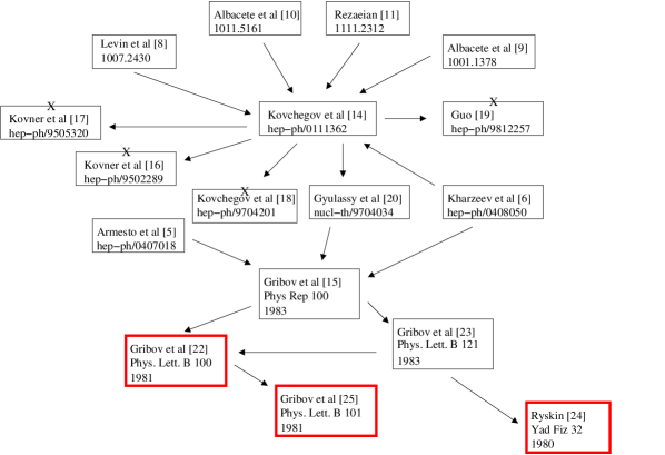
Figure 1: Some examples of the chain of references for the $k_{T}$-factorization formula (1). The boxes with crosses on top indicate references quoted for (1) where the equation is not even present in the paper. The boxes surrounded by a thick red line at the end of a chain are where a final proof or adequate justification of the formula would be expected to be found, yet, as documented in the text, this is not the case. Thus the chain of references does not lead to any source from which the validity of the formula could ultimately be verified. Only the arXiv numbers are shown for those papers that possess one, while for those who do not have arXiv numbers we show the journal name and volume for the publication.

A clear symptom that these are not merely abstract difficulties but are problems with practical impact is that the overall normalization factor differs dramatically between the references. See, for example, Eq. (40) in Kovchegov and Tuchin (2002) and Eq. (4.3) in Gribov et al. (1983a) — and notice that this difference in normalization does not appear to be commented on, let alone explained. The difference in normalization factors demonstrates that at least one of the presented factorization formulas is definitively wrong. (In the two appendices of the present paper, we will show that in fact the normalizations of both formulas appear to be wrong.) There are a number of difficult physical and mathematical issues that need to be addressed if one is to provide a fully satisfactory proof of a factorization formula. These issues go far beyond a mere normalization factor. But the existence of problems with the normalization factor is a diagnostic: it provides a clear and easily verifiable symptom that something has gone wrong. A minimum criterion for a satisfactory derivation is that it should be explicit enough to allow us to debug how the normalization factor arises.

At the top of our chart of references, Fig. 1, we have chosen some of the recent phenomenological applications Levin and Rezaeian (2010b); Albacete and Marquet (2010); Albacete and Dumitru (2010); Rezaeian (2012) that make use of (1). We also include some earlier highly cited phenomenological applications Armesto et al. (2005); Kharzeev et al. (2005). There exist a very great number of papers which make use of (1), so we include here only a representative few. As is indicated in the top part of Fig. 1, a central source that is given for (1) is the highly cited Ref. Kovchegov and Tuchin (2002). We thus ask whether we then can find a derivation of (1) in Kovchegov and Tuchin (2002).

That paper performs a calculation in a quasi-classical approximation of particle production in DIS using the dipole formalism (see the reference for the exact calculations that define this “quasi-classical” approximation). There actually is an implicit assumption of a factorized structure from the very start in this formalism (see Eqs. (1) and (7) in the reference). For our purposes it is important to notice what the exact statement is regarding (1), which can be found as Eq. (40) in Kovchegov and Tuchin (2002). (An unimportant difference is that in Kovchegov and Tuchin (2002), the $f$’s in (1) are instead written as $f/k_{T}^{2}$.) Prior to this equation, an equation for the production of gluons in DIS is derived, Eq. (39) in Kovchegov and Tuchin (2002). The exact statement just prior to stating (1) in the form of Eq. (40) in Kovchegov and Tuchin (2002) reads

The form of the cross section in Eq. (39) suggests that in a certain gauge or in some gauge invariant way it could be written in a factorized form involving two unintegrated gluon distributions merged by an effective Lipatov vertex.

There is no derivation of Eq. (1). Rather, this equation is stated as being the “usual form of the factorized inclusive cross section”, with the source being our Refs. Kovner et al. (1995a, b); Kovchegov and Rischke (1997); Guo (1999); Gyulassy and McLerran (1997). This is indicated by the arrows away from Ref. Kovchegov and Tuchin (2002) in Fig. 1. Furthermore, the paper then goes on to say that the results of the calculations actually appear to be “in disagreement with the factorization hypothesis”. (Our emphasis.) That is, Eq. (1) is actually false in the situation considered in Ref. Kovchegov and Tuchin (2002). Moreover, the calculations in the paper are for gluon production in DIS, whereas the papers that cite Ref. Kovchegov and Tuchin (2002) as a source for the factorization formula employ it in hadron-hadron collisions. Thus Ref. Kovchegov and Tuchin (2002) seems to be a particularly bad reference to cite for the validity of $k_{T}$-factorization, especially in nucleus-nucleus scattering, as is the case in Kharzeev et al. (2005); Levin and Rezaeian (2010a, b); Albacete and Marquet (2010); Albacete and Dumitru (2010); Rezaeian (2012).

To be fair, in a later paper Kharzeev et al. (2003), the authors of Kovchegov and Tuchin (2002) do propose a solution to the problem of the inconsistency of their calculations with $k_{T}$-factorization. The solution is that a different definition of the gluon distribution is needed — see the section of Kharzeev et al. (2003) that is titled “A tale of two gluon distribution functions”. But this simply reinforces our statement that Kovchegov and Tuchin (2002) is an entirely inappropriate reference to cite for $k_{T}$-factorization and its validity, at least not without considerable further explanation.

We next examine the sources Kovner et al. (1995a, b); Kovchegov and Rischke (1997); Guo (1999); Gyulassy and McLerran (1997) that Ref. Kovchegov and Tuchin (2002) itself cites for the factorization formula Eq. (1):

• In Refs. Kovner et al. (1995a, b) there actually exists no formula at all resembling (1), and those papers are not concerned with proving factorization. We indicate this fact in Fig. 1 by placing a cross on the references to Kovner et al. (1995a, b).

• In Ref. Kovchegov and Rischke (1997), there is one equation, (40), that has a somewhat similar structure to our (1). But in detail it is quite different, for example as regards the overall normalization and the number of powers of the strong coupling $g$, and the meaning of the functions inside the transverse-momentum integral. Thus this reference cannot be used to support a statement that (1) is the “usual form of the factorized inclusive cross section”.

• Reference Guo (1999) is concerned with a possible interpretation of the classical formula within perturbation theory using the DGLAP splitting kernels, but Eq. (1) is never present in the reference and we therefore again indicate this fact by placing a cross on the reference in Fig. 1.

• Finally, Ref. Gyulassy and McLerran (1997) does indeed contain Eq. (1), which is referred to as the “GLR formula” and is given by Eq. (65) in the reference. The origin of the formula is given as a review article by Gribov, Levin and Ryskin Gribov et al. (1983a) (GLR), as indicated in Fig. 1.

Thus to trace the origin of the $k_{T}$-factorization formula (1) we have come from the recent applications down to the GLR review Gribov et al. (1983a), via Ref. Kovchegov and Tuchin (2002).

So now let us turn to Ref. Gribov et al. (1983a). There the $k_{T}$-factorization formula appears as Eq. (4.3). But the numerical coefficient is $N_{c}/(2\pi)^{6}$, which is extremely different from the $2/C_{F}$ in our (1) and in Eq. (40) in Kovchegov and Tuchin (2002). In fact, as discussed in Sect. 4.4.1 of Avsar (2012), there appear many different formulas for the coefficient of (1). The choice in (1) corresponds to the choice in Kovchegov and Tuchin (2002) (and the majority of papers use this choice, as explained in section 4.4.1 of Avsar (2012)).

Indeed the normalization issue is referred to in the paper Gyulassy and McLerran (1997) that is citationally nearest to the GLR paper, in a section entitled “Comparison with GLR formula”. But the combination of (65) and (68) in Gyulassy and McLerran (1997) agrees with our (1) except for a previously mentioned redefinition of gluon densities by a factor of $k_{T}^{2}$. No mention is made of the dramatically different normalization factor in the GLR paper, even though the GLR paper is quoted as the source for the $k_{T}$-factorization formula. (Note that the formula in Gyulassy and McLerran (1997), like our (1), is for $d\sigma/d^{2}p_{T}dy$, whereas the formula in GLR is for the apparently different quantity $Ed\sigma/d^{3}p$; however, both these quantities are equal after applying the appropriate change of kinematic variable.)

In addition to the issue of normalization there are several other relatively minor differences between the versions of formula (1) among different papers. In Kharzeev et al. (2005) for example, the $k_{\perp}$ integral has $p_{\perp}$ as the upper limit, while other papers do not indicate such a limit. The use of such an upper limit is rather non-trivial because it does not treat the hadrons in a completely symmetric manner. Moreover, the integration measure is sometimes written $d^{2}k_{\perp}$ (e.g. Kovchegov and Tuchin (2002); Kharzeev et al. (2003); Armesto et al. (2005)) and sometimes $dk_{\perp}^{2}$ (e.g. Gribov et al. (1983a); Kharzeev et al. (2005)) so it is not clear what the correct prescription is. Finally, the coupling $\alpha_{s}$ is treated differently from paper to paper. In Gribov et al. (1983a) it is put inside the integral, with a $k_{T}$-dependent scale, while other papers write it as in (1), with a fixed $\alpha_{s}$ outside the integral. For someone well experienced with this area, these differences are likely to be unimportant. Thus the difference in the arguments of $\alpha_{s}$ could signal the difference between a strict leading-logarithm approximation and an idea about the likely result of an improved approximation.

But for an outsider to the topic, these differences can be quite bothersome, because it is not clear how they arise, or how significant they are, particularly when there is no comment on the differences. This is especially true in the absence of any derivations where one can locate the source of the differences.

At this point, an outsider should feel entitled to be able to examine a detailed step-by-step derivation, so as to be able to pinpoint where the error(s) is/are. That there is an error somewhere is absolutely demonstrated by the difference in normalization. As we have explained, there are no relevant derivations in the chronologically later papers whose citation chains led us back to Ref. Gribov et al. (1983a). But in Gribov et al. (1983a), we find no detailed derivation either. Just above that paper’s (4.3) there is a statement of what graphs are involved (with only a very brief explanation) and then a statement of what is supposed to be the resulting factorization formula. However, one is referred back to two previous papers Gribov et al. (1981a, 1983b) by the same authors, as indicated in Fig. 1.

But in these papers, we merely find that there is an assertion that certain graphs dominate, an assertion with a stated reason that certain other graphs cancel, and then a statement of the resulting formula. There is no detailed derivation, e.g., a derivation that is sufficiently detailed to make it manifest, for example, how the many factors of $2\pi$ that are ubiquitous in loop integrals organize themselves to give one or other of the very different normalization factors that are found in different version of the $k_{T}$-factorization formula.

It should also be mentioned that the assertions made in Refs. Gribov et al. (1983b, a) are based on the axial gauge where it is known that the unphysical singularities introduced in the gauge propagators do cause problems with divergences in the most natural simple definitions of the TMD parton densities, and additionally the contour deformations needed to prove factorization are blocked by these extra poles. See, e.g., (Collins, 2011, Chs. 13 & 14) for details of this. We find no indication in the cited references that such technical (yet crucial) issues are addressed.

In Gribov et al. (1983b), we read that the equation (with the normalization given in GLR, not the normalization that is currently accepted) “can easily be obtained in the QCD leading logarithmic approximation”, and the relevant references given are Gribov et al. (1981a); Ryskin (1980).

So we are now lead back to the papers Gribov et al. (1981a); Ryskin (1980). These two references are indicated by the red boxes in Fig. 1 and they thus constitute the two sources where one finally might expect to find a proof of (1), but presumably with a different normalization factor.

We first examine Gribov et al. (1981a), in which we have been told in Gribov et al. (1983b) that a derivation is to be found. Again we find no derivation. There is again just a statement of the diagrams involved and a statement of the resulting factorization formula. There is no derivation that can be debugged to check the normalization; there is not even any justification of why the particular graphs dominate. Neither is any statement given of the approximations involved. No prior references are given. Similarly in Ryskin (1980) we again find a short statement of the diagrams involved and of the factorization formula, but no detailed derivation or justification.

In Gribov et al. (1981a) it is also mentioned, below that paper’s Eq. (1), that the authors managed to calculate the relevant diagrams for the high-$p_{T}$ production of hadrons in Ref. Gribov et al. (1981b). We therefore also include this reference in Fig. 1. In Ref. Gribov et al. (1981b), the $k_{T}$-factorization formula is presented in the very last equation of the paper (un-numbered). It is, however, again simply stated without any derivation. Nor is any further reference or argument provided, and it is not at all clear what the definitions of the parton distributions are. It should also be noted that in Gribov et al. (1981b), an axial gauge is used for studying the leading graphs of high-$p_{T}$ processes. Thus one would here again expect the problems mentioned above that stem from unphysical gauge singularities. We find again no indication in the references that these problems are dealt with.

In Fig. 1, we have enclosed the boxes Gribov et al. (1981b); Ryskin (1980); Gribov et al. (1981a) in thick red lines. This denotes that they are at the end of the chains of citations, and that the derivations we should expect to find in them do not exist.

In the appendices of the present paper, we present a derivation of a $k_{T}$-factorization formula starting from what appear to be the same assumptions and approximations used by GLR. We get a quite different formula, as regards the normalization. Our proof gives what we intend to be enough detail that an outsider can verify the result. The assumptions and approximations are valid in a model that uses lowest-order graphs, so that our derivation is adequate to test whether a claimed result is actually true.

A summary of this section is that we find that regarding the important and widely used factorization formula (1), the principles (T1)–(T4) are violated very badly. A confusing chain of citations is present in the literature as shown in Fig. 1. By following the relevant references we are unable to find any paper where a proper derivation is provided. Moreover, the explicit definitions of the basic entities involved are not always clear, and differ from paper to paper (see also section 4 of Avsar (2012) for a more explicit discussion). It is therefore extremely important for progress in the field that all of recommendations (T1)–(T4) are adapted and maintained universally.

III Summary

Our principles (T1)–(T4) embody sensible standards and conventional norms for the presentation of work in theoretical physics. Suppose a paper uses, but does not derive, a particular formula of the status of the $k_{T}$-factorization formula (1) as a key part of its work. Then it is a normal and reasonable expectation that a reference should be given to where the formula is derived or otherwise justified. This we found to be badly violated, as summarized in Fig. 1.

For example, a main reference Kovchegov and Tuchin (2002) frequently given for (1) not merely failed to derive it but actually questioned its validity in the relevant context. Moreover, of the references that Kovchegov and Tuchin (2002) gives for the formula, most failed to even contain the formula. Backtracking through a chain of references where the formula does appear we eventually met a dead end: we could not actually find a useful derivation.

This is a quite disturbing situation. The formula in question is a key part of an important area of QCD phenomenology, and a superficial reading of the literature indicates that the formula appears to be accepted without question as the standard one. But closer examination fails to turn up a justification, at least not by following the normal and uncontroversial procedure of examining the references cited for the formula.

Of course, it may be that by a much wider search through the literature one can find an adequate justification of (1). But the point of a citation is to avoid a broad literature search: The reader just needs to go to the cited article(s) and find both the formula and its justification. Any substantial deviations from this expectation need explicit explanation.

A failure to find appropriate justification of a mainstream formula immediately raises the question as to whether the formula is correct. Recent work Collins and Qiu (2007); Rogers and Mulders (2010); Forshaw et al. (2012) finds violations of standard factorization in related situations, so ignoring the problems is both dangerous and can lead to failure to find correct consequences of QCD.

For a single paper whose citations are inadequate, it may be most appropriate to contact the author(s) to get corrected information. But in the present case, the problems are much more widespread, and need a more widespread concerted remedy. We also emphasize that we have identified other similar problems in the justification of related topics but for the sake of brevity we document here only the situation for one case: $k_{T}$-factorization for gluon production in hadron-hadron collisions.

We conjecture that one reason for the inadequate citations is that the $k_{T}$-factorization formula is regarded by its users as uncontroversial. Thus providing citations for it is a formality rather than a serious scientific exercise. We conjecture that a second reason is that there is substantial pressure, particularly on young scientists, to produce new results, and that it is regarded as counterproductive to actually check the validity of earlier results that are relied on to obtain the new results.

In addition, a disincentive to giving a full derivation is its length, if one makes explicit the details needed by a newcomer. For example, the derivation in the appendix of the present paper adds about $50\%$ to the paper’s length.

Our findings show that such tendencies need to be reduced for the health of our field; they greatly and unnecessarily impede the ability of other physicists to reproduce and verify the work. Insiders may have good reason to trust the formula, but workers in even closely related areas of QCD cannot check the results, at least not at all easily. The responsibility is not only on authors to justify their results adequately, but also on journal referees to check that results quoted in a new paper have actually been justified. Note that the problems we are finding are not at the level of a deep critique of a difficult proof; we find there is such an absence of derivation that there is not even a proof to critique.

Appendix A Derivation of the normalization factor of the $k_{T}$-factorization formula

Since we have been unable to find a derivation of the $k_{T}$-factorization formula (1) by following references for it, and since there is disagreement on the normalization factor, we provide here a simple derivation that gives the normalization.

The derivation starts from certain assumptions concerning the graphs and momentum regions that dominate. Since the assumptions are demonstrably incorrect at sufficiently high order in perturbation theory, as we will explain, the derivation cannot be completely correct as regards full QCD. Nevertheless, the derivation does apply to a simple Feynman graph model, and therefore unambiguously determines the appropriate value for the normalization, which differs from both of those in the standard references, (Gribov et al., 1983a, Eq. (4.3)) and (Kovchegov and Tuchin, 2002, Eq. (40)). Moreover, the assumptions we make are compatible with the stated starting point given in Gribov et al. (1983a, 1981a, b), so our derivation can be used to test the correctness of the factorization formula stated in those references.

Our derivation is a simplified version of a derivation that one of us gave in Ref. Avsar (2012).

A.1 Definition of process and gauge

We consider the cross section $d\sigma/d^{2}p_{T}dy$ for inclusive production of a gluon in a high-energy collision of unpolarized hadrons, where the gluon has transverse momentum $p_{T}$ and rapidity $y$. The kinematic region of interest is where $\Lambda\ll|p_{T}|\ll\sqrt{s}$ and $e^{y_{B}}\ll e^{y}\ll e^{y_{A}}$, where $\sqrt{s}$ is the center-of-mass energy, and $y_{A}$ and $y_{B}$ are the rapidities of the beam hadrons. We define $Q=|p_{T}|$, and let the momenta of the incoming hadrons be $P_{A}$ and $P_{B}$.

The aim is to obtain a factorized form for the cross section that is valid up to corrections that are a power of the small parameters $p_{T}/\sqrt{s}$, $e^{-(y-y_{B})}$, and $e^{-(y_{A}-y)}$.

We use light-front coordinates relative to the two beams, with the momentum of the detected gluon being

$$p=\left(p^{+},p^{-},p_{T}\right)=\left(\frac{Qe^{y}}{\sqrt{2}},\frac{Qe^{-y}}{\sqrt{2}},p_{T}\right).$$ (2)

Following Collins and Soper (1982, 1981), we use a time-like axial gauge $n\cdot\phi=0$. Here the symbol $\phi$ denotes the gluon field, since we use the usual symbol $A$ for another purpose. The gauge-fixing vector has the same rapidity as the detected gluon:

$$n\propto(e^{y},e^{-y},0_{T}),$$ (3)

Then the numerator of the gluon propagator has the form

$$-g^{\mu\nu}+\frac{k^{\mu}n^{\nu}+n^{\mu}k^{\nu}}{k\cdot n}-\frac{k^{\mu}k^{\nu}n^{2}}{(k\cdot n)^{2}}.$$ (4)

The point of this gauge is that for gluons of high positive rapidity it approximates the light-like axial gauge $\phi^{+}=0$ while for gluons of high negative rapidity it approximates the light-like axial gauge $\phi^{-}=0$. This happens since $k\cdot n\simeq k^{+}n^{-}$ when the rapidity of $k$ is large and positive, while $k\cdot n\simeq k^{-}n^{+}$ when the rapidity of $k$ is large and negative.

When various complications are ignored, each of these different light-like gauges gives an appropriately simple formulation of parton-model physics inside the corresponding beam hadron — see (Collins, 2011, Sec. 7.4) and references therein.

A.2 Assumptions

We make the following assumptions:

1. The cross section is dominated by (cut) graphs of the form of Fig. 2, where one gluon out of each hadron combines to form the observed gluon. Lines associated with the incoming hadrons are in the subgraphs $A$ and $B$.

2. We assume that the rapidities of lines in $A$ are substantially greater than the rapidity $y$ of the observed gluon, i.e., the rapidities in $A$ are at least $y+\Delta$, with $e^{\Delta}\gg 1$. This and the next assumption encode a key kinematic property used in BFKL physics.

3. Similarly the rapidities in $B$ are less than $y-\Delta$.

4. Transverse momenta in $A$ are of order $Q$ or smaller, and transverse momenta in $B$ are of order $Q$ or smaller.

5. We ignore the fact that a massless gluon is not a physical particle in real QCD, as opposed to low-order perturbation theory.

6. We ignore all other subtleties, e.g., that certain other graphical structures may be important, and can even break factorization Collins and Qiu (2007); Rogers and Mulders (2010); Forshaw et al. (2012).

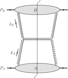
Figure 2: Graphs assumed to dominate for Eq. (1).

The assumptions are valid for the lowest-order graph in a perturbative model of high-energy quark-quark scattering, Fig. 3. In this graph, it is readily checked that the kinematic assumptions for the $A$ and $B$ subgraphs follow from the kinematic region chosen for the detected gluon. It can also be checked that other graphs of this order are power-suppressed in the gauge we have chosen, given that polarization vectors $\epsilon$ for the final-state gluon obey $\epsilon\cdot p=\epsilon\cdot n=0$.

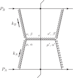
Figure 3: Lowest order example of Fig. 2. Here $\mu$, $\alpha$, etc, are Lorentz and color indices for the gluons attaching to the horizontal gluon line.

A.3 Cross section

At high-energy, the cross section from Fig. 2 is

$$\frac{d\sigma}{d^{2}p_{T}dy}=\frac{1}{2s}\int\frac{d^{4}k_{A}\,d^{4}k_{B}}{(2\pi)^{4}}\,\delta^{(4)}(k_{A}+k_{B}-p)\times\\ \times\frac{1}{16\pi^{3}}A^{\mu\mu^{\prime},\alpha\alpha^{\prime}}B^{\nu\nu^{\prime},\beta\beta^{\prime}}H_{\mu\mu^{\prime},\nu\nu^{\prime};\alpha\alpha^{\prime},\beta\beta^{\prime}}.$$ (5)

Here, $A^{\mu\mu^{\prime},\alpha\alpha^{\prime}}$ is the amplitude for the subgraph $A$ including the propagators for its two external gluons, as a function of the Lorentz and color indices of these gluons. It includes integrations over internal loop momenta and the momenta of the final-state particles of $A$. Similarly, $B^{\nu\nu^{\prime},\beta\beta^{\prime}}$ is for subgraph $B$. The factor

$$\frac{1}{16\pi^{3}}$$ (6)

arises from the Lorentz-invariant differential for the detected gluon:

$$\frac{d^{3}p}{(2\pi)^{3}2E_{p}}=\frac{dyd^{2}p_{T}}{16\pi^{3}},$$ (7)

given that the cross section is differential in $p_{T}$ and $y$. Finally, $H_{\mu\mu^{\prime},\nu\nu^{\prime};\alpha\alpha^{\prime},\beta\beta^{\prime}}$ is the factor for the central gluon:

$$H_{\mu\mu^{\prime},\nu\nu^{\prime};\alpha\alpha^{\prime},\beta\beta^{\prime}}=\sum_{\epsilon}g^{2}f_{\alpha\beta\gamma}f_{\alpha^{\prime}\beta^{\prime}\gamma}\times\\ \times\left[(k_{A}-k_{B})\cdot\epsilon g_{\mu\nu}+(k_{B}+p)_{\mu}\epsilon_{\nu}+(-p-k_{A})_{\nu}\epsilon_{\mu}\right]\times\\ \times\left[(k_{A}-k_{B})\cdot\epsilon g_{\mu^{\prime}\nu^{\prime}}+(k_{B}+p)_{\mu^{\prime}}\epsilon_{\nu^{\prime}}+(-p-k_{A})_{\nu^{\prime}}\epsilon_{\mu^{\prime}}\right].$$ (8)

The sum is over two independent orthonormal polarization vectors for the gluon. In a frame in which $p_{T}$ is along the $x$-axis:

$$p=Q\left(\frac{e^{y}}{\sqrt{2}},\frac{e^{-y}}{\sqrt{2}},1,0\right),$$ (9)

we can choose

$$\epsilon_{1}=(0,0,0,1)~{}\mbox{and}~{}\epsilon_{2}=\left(e^{y},-e^{-y},0,0\right)/\sqrt{2}$$ (10)

as the independent polarization vectors.

To keep track of the dependence of calculations on the gauge group, we will assume that the gauge group is SU($N_{c}$).

A.4 Leading-power approximations

We now make approximations suitable for the kinematic region that we have assumed.

First we need the size of the components of the momenta $k_{A}$ and $k_{B}$ of the gluons coming out of $A$ and $B$:

$$k_{A} =\left(\frac{Qe^{y}}{\sqrt{2}}+O(Qe^{y-\Delta}),~{}O(Qe^{-y-\Delta}),~{}k_{A,T}\right),$$ (11)

$$k_{B} =\left(O(Qe^{y-\Delta}),~{}\frac{Qe^{-y}}{\sqrt{2}}+O(Qe^{-y-\Delta}),~{}k_{B,T}\right).$$ (12)

The components $k_{A}^{-}$ and $k_{B}^{+}$ are small relative to the corresponding components of $p$, since the components of $k_{A}$ and $k_{B}$ cannot exceed the typical values for momenta in $A$ and $B$; the sizes of momenta in $A$ and $B$ are governed by our assumed separation of rapidity between $A$, $B$ and the gluon $p$. Then momentum conservation at the three-gluon vertex ensures that $k_{A}^{+}$ and $k_{B}^{-}$ equal $p^{+}$ and $p^{-}$, up to small corrections.

Next consider the line for one of the external gluon lines of $A$. It connects a subgraph $H$ characterized by rapidity $y$ to a subgraph $A$ with rapidity $y+\Delta$, and we write the relevant part of the graph as

$$a^{\lambda}\,N_{\lambda\mu}(k_{A})\,h^{\mu}.$$ (13)

Here $N_{\lambda\mu}$ is the numerator of the gluon propagator, while $a$ and $h$ correspond to the rest of the $A$ subgraph and to the $H$ subgraph. We treat $h^{\mu}$ and $a^{\lambda}$ as being obtained by a boost from a situation with zero rapidity, and therefore we obtain relative sizes for the components:

$$a=(a^{+},a^{-},a_{T}) \sim\mbox{const.}\times(e^{y+\Delta},e^{-y-\Delta},1),$$ (14)

$$h \sim\mbox{const.}\times(e^{y},e^{-y},1).$$ (15)

We use the sizes given in (11) to determine that the sum over components in (13) is dominated by $\lambda=+$ and the transverse components in $\mu$:

$$-a^{+}N^{-i}h^{i}.$$ (16)

A corresponding calculation is then applied to each of the gluons connecting the central gluon to the $B$ subgraph.

Finally we observe that $k_{A}^{+}$ and $k_{B}^{-}$ differ from $Qe^{y}/\sqrt{2}$ and $Qe^{-y}/\sqrt{2}$ by an amount that is small compared with the corresponding components of momenta in $A$ and $B$. Thus in $A$ and $B$ we can replace $k_{A}^{+}$ by $Qe^{y}/\sqrt{2}$, and $k_{B}^{-}$ by $Qe^{-y}/\sqrt{2}$.

We then find that, given our assumptions, the cross section is given by

$$\frac{d\sigma}{d^{2}p_{T}dy}=\frac{\pi}{2s}\int d^{2}k_{A,T}\int\frac{dk_{A}^{-}}{(2\pi)^{4}}\int\frac{dk_{B}^{+}}{(2\pi)^{4}}\times\\ \times A^{ii^{\prime},\alpha\alpha^{\prime}}B^{jj^{\prime},\beta\beta^{\prime}}H^{ii^{\prime},jj^{\prime};\alpha\alpha^{\prime},\beta\beta^{\prime}},$$ (17)

where the integrals and factors of $2\pi$ are arranged to correspond to those in the definition of a gluon density, as we will see.

A.5 Gluon density

If there were no complications, the natural method to define a number density of a parton is by the hadron expectation value of the number operator in the sense of light-front quantization. The basic ideas were worked out by Bouchiat, Fayet, and Meyer Bouchiat et al. (1971) and by Soper Soper (1977), although these papers do not contain actual formulas for transverse-momentum-dependent parton densities in terms of hadron matrix elements of field operators. In light-front quantization and light-front gauge, this gives the gluon density as

$$P(x,k_{T})=\frac{xP^{+}}{(2\pi)^{3}}\int dw^{-}d^{2}w_{T}\,e^{-ixP^{+}w^{-}+ik_{T}\cdot w_{T}}\times\\ \times\langle P|\phi^{i,\alpha}(0,w^{-},w_{T})\phi^{i,\alpha}(0)|P\rangle,$$ (18)

where $\phi^{\mu,\alpha}$ denotes the gluon field operator. This definition is equivalent to Eq. (2.3) of Collins and Soper (1982) when the light-cone gauge $\phi^{+}=0$ is used, which we will now show to be appropriate in the approximation we are using.

If gluon momenta all have high rapidity, then $k\cdot n=k^{+}n^{-}\left(1+\frac{k^{-}}{k^{+}}\frac{n^{+}}{n^{-}}\right)\simeq k^{+}n^{-}$ in the gluon propagator, where the neglect of $k^{-}n^{+}/(k^{+}n^{-})$ relative to unity follows because the rapidity of $k$ is much higher than that of $n$. Note that for the gluon momentum $k_{A}$ entering the hard scattering, the size of the plus component is appropriate for the hard scattering, i.e., $k_{A}^{+}\sim Qe^{y}$, but the minus component is appropriate for subgraph $A$, i.e., $k_{A}^{-}\sim Qe^{-y+\Delta}$, so that $k_{A}$ has effectively rapidity of about $y+\Delta$.

Hence in the gluon density, time-like axial gauge is equivalent to $\phi^{+}=0$ gauge to leading power. The above definition then gives

$$P(x,k_{T})=k^{+}\int\frac{dk^{-}}{(2\pi)^{4}}A^{ii,\alpha\alpha}(k,P).$$ (19)

The normalization of the above definition is that $P(x,k_{T})$ would be a number density of gluons in $x$ and $k_{T}$, if we ignored the complications present in higher order corrections in QCD. The corresponding quantity in the $k_{T}$-factorization formula (1) is actually a momentum density. Therefore, in the above formulas, we follow Refs. Soper (1979); Collins and Soper (1982), and use $P(x,k_{T})$ to denote the number density, rather than the more common notation $f(x,k_{T})$.

Of course, as explained in (Collins, 2011, Chs. 13 & 14) the light-cone-gauge definition has problems, because of rapidity divergences and other issues, and even the definition with a non-light-like axial gauge has trouble. So the definitions have to be modified to be suitable for full QCD. But within the approximation used here, the simplest definition is adequate.

A.6 Factorization

We next recall that in the small-$x$ limit and in the approximation we use here, only the term (16) in the lines for the external gluons of $A$ is important. So for each gluon line there is a factor of the vector transverse momentum multiplying a rotationally invariant quantity. Moreover with a color-singlet or a color-averaged beam, the dependence of $A$ on color is proportional to $\delta_{\alpha\alpha^{\prime}}$.

Thus for the $A$ factor in (17), we have

$$\int\frac{dk_{A}^{-}}{(2\pi)^{4}}A^{ii^{\prime},\alpha\alpha^{\prime}} =\frac{k_{A}^{i}k_{A}^{i^{\prime}}}{|k_{A,T}|^{2}}\frac{\delta_{\alpha\alpha^{\prime}}}{N_{c}^{2}-1}\int\frac{dk_{A}^{-}}{(2\pi)^{4}}A^{jj,\beta\beta}$$

$$=\frac{k_{A}^{i}k_{A}^{i^{\prime}}}{|k_{A,T}|^{2}}\frac{\delta_{\alpha\alpha^{\prime}}}{N_{c}^{2}-1}\frac{1}{k_{A}^{+}}P(x_{A},k_{A,T}).$$ (20)

Here the factors of $k_{A}^{i}$ and $k_{A}^{i^{\prime}}$ arise from the axial-gauge gluon propagator as it is used in (16), while $x_{A}=Qe^{y}/(\sqrt{2}p_{A}^{+})=Qe^{y}/\sqrt{s}$ (in the overall center-of-mass frame). An exactly similar result applies to the $B$ subgraph, with $x_{B}=Qe^{-y}/(\sqrt{2}p_{B}^{-})=Qe^{-y}/\sqrt{s}$. Substituting these results in (17) gives

$$\frac{d\sigma}{d^{2}p_{T}dy}=\frac{\pi}{x_{A}x_{B}s^{2}(N_{c}^{2}-1)^{2}}\int d^{2}k_{A,T}\,P_{A}(x_{A},k_{A,T})\times\\ \times P_{B}(x_{B},p_{T}-k_{A,T})\frac{k_{A}^{i}k_{A}^{i^{\prime}}k_{B}^{j}k_{B}^{j^{\prime}}H^{ii^{\prime},jj^{\prime};\alpha\alpha,\beta\beta}}{|k_{A,T}|^{2}|k_{B,T}|^{2}}.$$ (21)

Performing the algebra in the $H$ factor, and making approximations valid to leading power in $e^{-\Delta}$ then gives the following factorization formula

$$\frac{d\sigma}{d^{2}p_{T}dy}=\frac{2\pi^{2}\alpha_{s}}{C_{F}\,p_{T}^{2}}\int d^{2}k_{A,T}\,x_{A}P_{A}(x_{A},k_{A,T})\times\\ \times x_{B}P_{B}(x_{B},p_{T}-k_{A,T}),$$ (22)

with $\alpha_{s}=g^{2}/(4\pi)$ and $C_{F}=(N_{c}^{2}-1)/(2N_{c})$, as usual. Notice that each gluon density has been multiplied by a factor of the corresponding $x$ value, and that this compensated a change from $1/s$ to $1/p_{T}^{2}$ in the pre-factor.

This factorization formula is to be compared with the formula stated earlier, (1), which has the normalization given in (Kovchegov and Tuchin, 2002, Eq. (40)). Evidently in that formula, the gluon densities are to be interpreted as momentum densities rather than number densities, i.e., $f(x,k_{T})=xP(x,k_{T})$. But there is also a factor of $\pi^{2}$ missing.

A.7 Why the proof is insufficient

Our derivation of the factorization formula (22) relied on certain assumptions, which are not in general true in QCD. However they are true for the lowest-order graph, so that our derivation gives the correct normalization factor. At a minimum the proof needs enhancement if the result is to be regarded as actually derivable in full QCD. We now explain some of the difficulties.

In the first place the definition of the gluon density needs to be changed. Already, it was seen in Collins and Soper (1982, 1981) that the natural definition of a TMD quark density in light-cone gauge has rapidity divergences. This was corrected by the use of non-light axial gauge. But even this has problems (Bacchetta et al., 2008, App. A). A satisfactory gauge-invariant definition for a TMD quark density was recently given by one of us in (Collins, 2011, Chs. 13 & 14), and the definition can be extended in a reasonably natural way to a TMD gluon density. However, the treatment in Collins (2011) did not cover the additional issues that arise at small $x$.

In general, many more kinds of graph and momentum region contribute. If factorization is to hold, various summations and cancellations have to be employed. Moreover some of the cancellations involve issues of relativistic causality — see Bodwin (1985); Collins et al. (1988) — which is broken graph-by-graph by the $k\cdot n$ denominators in the axial-gauge gluon propagator — see (4). Use of the Feynman gauge increases the number of graphical structures and regions to be considered.

Furthermore, it has recently been found that factorization is actually violated in some significant situations in hadron-hadron collisions Collins and Qiu (2007); Rogers and Mulders (2010); Forshaw et al. (2012). While these particular examples do not include the particular process discussed in the present paper, they do show that claimed proofs of factorization need careful attention to ensure that they actually work.

Appendix B Testing the normalization factor

The argument that derives the normalization of the $k_{T}$-factorization formula is somewhat long. Since the result disagrees with both of the standard formulas to be found in the literature, it is useful to find some elementary tests to verify our result.

In our formula (22) the factors of $\pi^{2}$ are different from those in both (Gribov et al., 1983a, Eq. (4.3)) and (Kovchegov and Tuchin, 2002, Eq. (40)). The group theory factor $1/C_{F}$ does agree with that in Kovchegov and Tuchin (2002), but disagrees with the factor $N_{c}$ in Gribov et al. (1983a), which is written there simply as $N$.

We do the verification by determining how the powers of $\pi$ and the $N_{c}$ dependence arise in the lowest-order graph Fig. 3 for the cross section and in the lowest-order graph for the gluon density. We will show how this immediately gives the power of $\pi$ and the $N_{c}$ dependence in the prefactor in the factorization formula (22). In the lowest-order graphs and in $n\cdot\phi=0$ gauge, all our assumptions are valid, and agree with the starting point in GLR Gribov et al. (1983a), so at lowest-order there is no ambiguity as to the correct result.

B.1 Power of $\pi$

In the cross section, the integral over the plus and minus components of the loop momentum are performed using the mass-shell delta-functions for the spectator quarks. After the standard kinematic approximations these give simple algebraic calculations, and hence no factors of $\pi$. There remains a two-dimensional transverse momentum integral which is unchanged between the cross section calculation and the factorization formula. From the differential (7), there is a $1/\pi^{3}$ for each of the 3 final-state particles, and there is a $\pi^{4}$ associated with the delta-function for overall momentum conservation. This gives an overall factor of $1/\pi^{5}$ in the cross section.

In the one-loop gluon density the definition itself contains an overall factor of $1/\pi^{4}$, and there is a factor of $\pi$ from the $2\pi\delta((p-k)^{2})$ that puts the spectator quark on-shell. This gives an overall factor of $1/\pi^{3}$.

To match these powers of $\pi$, the coefficient of the two gluon densities in the factorization formula for the cross section has a factor of $\pi$. Since $\alpha_{s}=g^{2}/(4\pi)$, we need a factor $\pi^{2}$ multiplying $\alpha_{s}$, which is exactly what we have in (22). The factorization formulas in both of Refs. Gribov et al. (1983a); Kovchegov and Tuchin (2002) have a different power of $\pi$ and are therefore wrong.

B.2 Dependence on $N_{c}$

We now ask for the dependence on $N_{c}$ when the gauge-group is SU($N_{c}$). We choose the quarks in Fig. 3 to be in the fundamental representation, and we choose the cross section to be averaged over the colors of the initial-state quarks. In a correct factorization formula, the coefficient is independent of the nature of the beam particles, of course, so these choices for the beams are purely for calculational convenience.

Then the group theory factor for the graph for the cross section has the form

$$\frac{1}{N_{c}^{2}}\mbox{tr}(t_{\alpha}t_{\alpha^{\prime}})\mbox{tr}(t_{\beta}t_{\beta^{\prime}})f_{\alpha\beta\gamma}f_{\alpha^{\prime}\beta^{\prime}\gamma}=\frac{N_{c}^{2}-1}{4N_{c}}.$$ (23)

Here repeated indices are summed, as usual, and the result was obtained by use of the formulas $\mbox{tr}(t_{\alpha}t_{\alpha^{\prime}})=\frac{1}{2}\delta_{\alpha\alpha^{\prime}}$, $f_{\alpha\beta\gamma}f_{\alpha\beta^{\prime}\gamma}=N_{c}\delta_{\beta\beta^{\prime}}$, and $\delta_{\gamma\gamma}=N_{c}^{2}-1$.

Each parton density has a group-theory factor

$$\frac{1}{N_{c}}\mbox{tr}(t_{\alpha}t_{\alpha})=C_{F}=\frac{N_{c}^{2}-1}{2N_{c}}.$$ (24)

The coefficient in the factorization formula therefore has a factor

$$\frac{N_{c}^{2}-1}{4N_{c}}\frac{1}{C_{F}^{2}}=\frac{N_{c}}{N_{c}^{2}-1}=\frac{1}{2C_{F}},$$ (25)

in agreement with our factorization formula in (22) and with the one in Kovchegov and Tuchin (2002), but in disagreement with Gribov et al. (1983a).

References

- Kraml et al. (2012) S. Kraml, B.C. Allanach, M. Mangano, H.B. Prosper, S. Sekmen, et al., “Searches for new physics: Les Houches recommendations for the presentation of LHC results,” (2012), arXiv:1203.2489 [hep-ph] .
- Collins (2011) J. C. Collins, Foundations of Perturbative QCD (Cambridge University Press, Cambridge, UK, 2011).
- Note (1) Mark Strikman in a personal communication remarked that it is an interesting question as to whether the literature on Regge theory meets these standards sufficiently well. But we do not wish to answer that particular question here.
- Kharzeev et al. (2003) Dmitri Kharzeev, Yuri V. Kovchegov, and Kirill Tuchin, “Cronin effect and high suppression in pA collisions,” Phys.Rev. D68, 094013 (2003), arXiv:hep-ph/0307037 [hep-ph] .
- Armesto et al. (2005) Nestor Armesto, Carlos A. Salgado, and Urs Achim Wiedemann, “Relating high-energy lepton-hadron, proton-nucleus and nucleus-nucleus collisions through geometric scaling,” Phys.Rev.Lett. 94, 022002 (2005), arXiv:hep-ph/0407018 [hep-ph] .
- Kharzeev et al. (2005) Dmitri Kharzeev, Eugene Levin, and Marzia Nardi, “Color glass condensate at the LHC: Hadron multiplicities in , and collisions,” Nucl.Phys. A747, 609–629 (2005), arXiv:hep-ph/0408050 [hep-ph] .
- Levin and Rezaeian (2010a) Eugene Levin and Amir H. Rezaeian, “Gluon saturation and inclusive hadron production at LHC,” Phys. Rev. D82, 014022 (2010a), arXiv:1005.0631 [hep-ph] .
- Levin and Rezaeian (2010b) Eugene Levin and Amir H. Rezaeian, “Hadron multiplicity in and collisions at LHC from the color glass condensate,” Phys. Rev. D82, 054003 (2010b), arXiv:1007.2430 [hep-ph] .
- Albacete and Marquet (2010) Javier L. Albacete and Cyrille Marquet, “Single inclusive hadron production at RHIC and the LHC from the color glass condensate,” Phys.Lett. B687, 174–179 (2010), arXiv:1001.1378 [hep-ph] .
- Albacete and Dumitru (2010) Javier L. Albacete and Adrian Dumitru, “A model for gluon production in heavy-ion collisions at the LHC with rcBK unintegrated gluon densities,” (2010), arXiv:1011.5161 [hep-ph] .
- Rezaeian (2012) Amir H. Rezaeian, “Charged particle multiplicities in pA interactions at the LHC from the color glass condensate,” Phys.Rev. D85, 014028 (2012), arXiv:1111.2312 [hep-ph] .
- Tribedy and Venugopalan (2011) Prithwish Tribedy and Raju Venugopalan, “QCD saturation at the LHC: comparisons of models to p+p and A+A data and predictions for p+Pb collisions,” (2011), arXiv:1112.2445 [hep-ph] .
- Abelev et al. (2010) B Abelev et al. (ALICE Collaboration), “Charged-particle multiplicity density at mid-rapidity in central Pb-Pb collisions at TeV,” Phys.Rev.Lett. 105, 252301 (2010), arXiv:1011.3916 [nucl-ex] .
- Kovchegov and Tuchin (2002) Yuri V. Kovchegov and Kirill Tuchin, “Inclusive gluon production in DIS at high parton density,” Phys. Rev. D65, 074026 (2002), arXiv:hep-ph/0111362 .
- Gribov et al. (1983a) L. V. Gribov, E. M. Levin, and M. G. Ryskin, “Semihard processes in QCD,” Phys. Rept. 100, 1–150 (1983a).
- Kovner et al. (1995a) Alex Kovner, Larry D. McLerran, and Heribert Weigert, “Gluon production from non-abelian Weizsacker-Williams fields in nucleus-nucleus collisions,” Phys.Rev. D52, 6231–6237 (1995a), arXiv:hep-ph/9502289 [hep-ph] .
- Kovner et al. (1995b) Alex Kovner, Larry D. McLerran, and Heribert Weigert, “Gluon production at high transverse momentum in the McLerran-Venugopalan model of nuclear structure functions,” Phys.Rev. D52, 3809–3814 (1995b), arXiv:hep-ph/9505320 [hep-ph] .
- Kovchegov and Rischke (1997) Yuri V. Kovchegov and Dirk H. Rischke, “Classical gluon radiation in ultrarelativistic nucleus-nucleus collisions,” Phys.Rev. C56, 1084–1094 (1997), arXiv:hep-ph/9704201 [hep-ph] .
- Guo (1999) Xiao-feng Guo, “Gluon minijet production in nuclear collisions at high-energies,” Phys.Rev. D59, 094017 (1999), arXiv:hep-ph/9812257 [hep-ph] .
- Gyulassy and McLerran (1997) M. Gyulassy and Larry D. McLerran, “Yang-Mills radiation in ultrarelativistic nuclear collisions,” Phys.Rev. C56, 2219–2228 (1997), arXiv:nucl-th/9704034 [nucl-th] .
- Avsar (2012) Emil Avsar, “TMD factorization and the gluon distribution in high energy QCD,” (2012), arXiv:1203.1916 [hep-ph] .
- Gribov et al. (1981a) L. V. Gribov, E. M. Levin, and M. G. Ryskin, “High hadrons in the pionization region in QCD,” Phys. Lett. B100, 173–176 (1981a).
- Gribov et al. (1983b) L. V. Gribov, E. M. Levin, and M. G. Ryskin, “Large- processes as a main source of hadrons at very high-energies,” Phys. Lett. B121, 65–71 (1983b).
- Ryskin (1980) M.G. Ryskin, “Hadron productin with large transverse momentum in the pionization region and the vacuum singularity in QCD,” Sov. J. Nucl. Phys. 32, 133–140 (1980), yad. Fiz. 32, 259-274 (1980).
- Gribov et al. (1981b) L.V. Gribov, E.M. Levin, and M.G. Ryskin, “Extending the QCD leading logs up to reggeon field theory,” Phys.Lett. B101, 185 (1981b).
- Collins and Qiu (2007) John Collins and Jian-Wei Qiu, “ factorization is violated in production of high-transverse-momentum particles in hadron-hadron collisions,” Phys. Rev. D75, 114014 (2007), arXiv:0705.2141 [hep-ph] .
- Rogers and Mulders (2010) Ted C. Rogers and Piet J. Mulders, “No generalized TMD-factorization in hadro-production of high transverse momentum hadrons,” Phys.Rev. D81, 094006 (2010), arXiv:1001.2977 [hep-ph] .
- Forshaw et al. (2012) Jeffrey R. Forshaw, Michael H. Seymour, and Andrzej Siodmok, “On the breaking of collinear factorization in QCD,” (2012), arXiv:1206.6363 [hep-ph] .
- Note (2) In addition, the foundational work on a topic, which may be decades old, may give the key ideas, but not the extra steps to put results in the form in which they are later found to be most useful and convenient. It may be that these extra steps are known privately to insiders but that they do not appear in the papers that it is most natural to cite. We give an explicit example in Sec. A.5. This phenomenon can explain the problems with the citations, but it leaves unchanged the readers’ difficulty of reproducing results.
- Collins and Soper (1982) John C. Collins and Davison E. Soper, “Parton distribution and decay functions,” Nucl. Phys. B194, 445 (1982).
- Collins and Soper (1981) John C. Collins and Davison E. Soper, “Back-to-back jets in QCD,” Nucl. Phys. B193, 381 (1981).
- Bouchiat et al. (1971) C. Bouchiat, P. Fayet, and P. Meyer, “Galilean invariance in the infinite momentum frame and the parton model,” Nucl. Phys. B34, 157–176 (1971).
- Soper (1977) D. E. Soper, “The parton model and the Bethe-Salpeter wave function,” Phys. Rev. D15, 1141–1149 (1977).
- Note (3) This gives an example of the difficulty referred to in footnote References.
- Soper (1979) D. E. Soper, “Partons and their transverse momenta in QCD,” Phys. Rev. Lett. 43, 1847–1851 (1979).
- Note (4) Note that the definition in Collins (2011) is for a TMD quark density. For a TMD gluon density, one makes the same adjustments as are used to get the formula for an integrated gluon density from the formula for an integrated quark density.
- Bacchetta et al. (2008) Alessandro Bacchetta, Daniel Boer, Markus Diehl, and Piet J. Mulders, “Matches and mismatches in the descriptions of semi-inclusive processes at low and high transverse momentum,” JHEP 08, 023 (2008), arXiv:0803.0227 [hep-ph] .
- Bodwin (1985) G. T. Bodwin, “Factorization of the Drell-Yan cross-section in perturbation theory,” Phys. Rev. D31, 2616–2642 (1985), erratum: D34, 3932 (1986).
- Collins et al. (1988) J. C. Collins, D. E. Soper, and G. Sterman, “Soft gluons and factorization,” Nucl. Phys. B308, 833–856 (1988).