Kinetic temperatures toward X1/X2 orbit interceptions regions and Giant Molecular Loops in the Galactic center region

Abstract

Context. It is well known that the kinetic temperatures, $T_{\rm kin}$, of the molecular clouds in the Galactic center region are higher than in typical disk clouds. However, the $T_{\rm kin}$ of the molecular complexes found at higher latitudes towards the giant molecular loops in the central region of the Galaxy is so far unknown. The gas of these high latitude molecular clouds (hereafter referred to as “halo clouds”) is located in a region where the  gas in the disk may interact with the gas in the halo in the Galactic center region.

Aims. To derive $T_{\rm kin}$ in the molecular clouds at high latitude and understand the physical process responsible for the heating of the molecular gas both in the Central Molecular Zone (the concentration of molecular gas in the inner $\sim 500$ pc) and in the giant molecular loops.

Methods. We measured the metastable inversion transitions of NH₃ from $(J,K)=(1,1)$ to $(6,6)$ toward six positions selected throughout the Galactic central disk and halo. We used rotational diagrams and large velocity gradient (LVG) modeling to estimate the kinetic temperatures toward all the sources. We also observed other molecules like SiO, HNCO, CS, C³⁴S, C¹⁸O, and ¹³CO, to derive the densities and to trace different physical processes (shocks, photodissociation, dense gas) expected to dominate the heating of the molecular gas

Results. We derive for the first time $T_{\rm kin}$ of the high latitude clouds interacting with the disk in the Galactic center region. We find high rotational temperatures in all the observed positions. We derive two kinetic temperature components ($\sim 150$ K and $\sim 40$ K) for the positions in the Central Molecular Zone, and only the warm kinetic temperature component for the clouds toward the giant molecular loops. The fractional abundances derived from the different molecules suggest that shocks provide the main heating mechanism throughout the Galactic center, also at high latitudes.

1 Introduction

The interstellar molecular gas in the Galactic center (GC) region (i.e., in the inner $\sim 1$ kpc of the Galaxy) shows higher kinetic temperatures, $T_{\rm kin}$, than typical disk clouds. Using metastable inversion transitions of para-NH₃, Güsten et al. (1981) derived kinetic temperatures in the range of 50-120 K towards Sgr A. Mapping the (1,1), (2,2), and (3,3) inversion transitions of NH₃, Morris et al. (1983) found high kinetic temperatures (30-60 K) towards the denser portions of the GC region. Observing more highly excited NH₃ inversion lines, Mauersberger et al. (1986a) and Hüttemeister et al. (1993b) obtained kinetic temperatures $T_{\rm kin}\geq 100$ K in all clouds in the GC including Sgr B2 region. Similarly high temperatures were also found in the central regions of nearby galaxies, (e.g., Mauersberger et al. 2003). From metastable, i.e. $J=K$, inversion transitions of NH₃ toward 36 clouds throughout the GC region, Hüttemeister et al. (1993a) suggested that in addition to a warm component there is also a “cool gas component” with $T_{\rm kin}\sim 20-30$ K. The extended warm component in the GC of $\sim 200$ K is not coupled with the dust (Rodríguez-Fernández et al. 2002; Odenwald & Fazio 1984; Cox & Laureijs 1989, $T_{\rm dust}<40$ K, ). High dust temperatures ($T_{\rm dust}\sim 80$ K) are only seen toward the Sgr B2 molecular cloud, which is claimed to be an anomalous region, with recent massive star formation (Bally et al. 2010). So far, to our knowledge, the $T_{\rm kin}$ of molecular clouds has never been determined either at higher latitudes towards the Giant Molecular Loops (GMLs, Fukui et al. 2006), or in the forbidden and/or high velocity components, explained by the barred potential model as X1 orbits.
The kinetic temperature of the molecular gas results from the balance of heating and cooling. Molecular clouds cool down by the collisional excitation of molecules and atoms followed by the radiative emission of this energy from the cloud (Hollenbach 1988). For the physical conditions present in the GC, the cooling is dominated by H₂ and CO, while Hüttemeister et al. (1993a) propose that the dust in the GC region is also an important cooling agent.
Dust heated via stars cannot heat gas sufficiently, just because the gas is warmer than the dust. Several heating mechanisms for the GC region have been proposed, as e.g., heating by cosmic rays (Güsten et al. 1981; Morris et al. 1983); heating by X-rays (Watson et al. 1981; Nagayama et al. 2007); magnetic ion-slipping (Scalo 1977). The dissipation of mechanical supersonic turbulence through shocks has been proposed for the GC (Fleck 1981; Wilson et al. 1982; Mauersberger et al. 1986a). The shocks can be produced by several phenomena: supernova or hypernova explosions (Tanaka et al. 2007); response of the gas in a barred potential model (Binney et al. 1991); and when the gas in the GMLs flows down their sides along the magnetic field lines, and joins with the gas layer of the Galactic plane generating shock front at the “foot points” of the loops (Fukui et al. 2006).

NH₃ is one of the best thermometers for measuring the gas kinetic temperatures in molecular clouds (see, Ho & Townes 1983). Observing several metastable inversion transitions, one can determinate the kinetic temperature of the molecular clouds.

In this paper, we derive for the first time the kinetic temperatures of the molecular clouds in the disk-halo interaction regions (foot points of the GMLs and positions where the X1 orbits intercept X2 orbits in a barred potential). We use metastable inversion transitions of NH₃ and other molecular tracers (SiO, HNCO, CS) to estimate the kinetic temperatures and densities, and discuss the heating mechanisms of the molecular gas in the GC.

2 Observations

2.1 Effelsberg observations

We observed the metastable inversion transition of NH₃ $(J,K)=(1,1)$, $(2,2)$, $(3,3)$, $(4,4)$, $(5,5)$, and $(6,6)$ using the Effelsberg 100m telescope in April 2010, and April 2011. We used the primary focus $\lambda=1.3$ cm ($18-26$ GHz) receiver, which has 2 linear polarizations, and a Fast Fourier Transform Spectrometer (FFTS) in the “broad IF band” mode with a bandwidth of 500 MHz, providing an effective spectral resolution of 49.133 kHz or 0.386  km s^-1. We observed the $(1,1)$, $(2,2)$ and $(3,3)$ line simultaneously, with a band centered at 23.783 GHz, and the $(4,4)$ and $(5,5)$ line in a second setup (centered at 24.336 GHz). The $(6,6)$ was observed in the third setup, centered at 25.056 GHz, using the 100 MHz bandwidth FFTS spectrometer, which provides an effective spectral resolution of 9.827 kHz or 0.073  km s^-1. The beam width of the telescope at 23.7 GHz is 42.2”. The spectra were observed in position switching mode, with the emission-free reference positions from Riquelme et al. (2010b), which were checked in the first setup, where the most intense lines are detected. Each position was observed for 12 min in the first setup, 24 min in the second setup, and 32 min in the third setup. The calibration in Effelsberg was done by the periodic injection of a constant signal (noise cal). To convert the data to $T_{\rm A}^{*}$ we corrected for the noise-cal (in K), opacity and elevation dependent antenna gain. The uncertainty in the calibration is of the order of $5-10\%$. The main beam temperatures, T_MB, were obtained by using $T_{\rm MB}=T^{*}_{\rm A}\cdot\frac{1}{{\rm Beff}}$, where the beam efficiency, ${\rm Beff}$, is $0.52$ at $24$ GHz. The pointing was checked every two hours against the source 1833-212, providing an accuracy of better than $10^{\prime\prime}$.
In this work, we observe the positions selected in Riquelme et al. (2010a). To avoid confusion, we use the notation of that work. The “Central Molecular Zone” (CMZ, Morris & Serabyn 1996) corresponds to the region about $-0{{}^{\circ}}.5<l<1{{}^{\circ}}.5$. Since the clouds of the CMZ are aligned along the Galactic plane within b$\sim$ 0^∘, this can be viewed as an extension of the Galactic disk, towards galactocentric radii $<1$ kpc and will therefore be called “disk”. When one observed position (from those called “disk”) have kinematical components associated to both, the X1 and the X2 orbits in the barred potential model, we called them explicitly as ‘Disk X1” and “Disk X2”. The source “Disk 2” which corresponds to Sgr B2, is located toward the X2 orbits. Since this source does not have the velocity components associated to the X1 orbits, we just call this source as “Disk”. Gas toward the GMLs regions is labeled as “halo” in this paper, to differentiate them from the molecular clouds in the Galactic plane. This does not imply that the findings in this paper can be applied to the disk or the halo of the Galaxy as a whole, because all of the positions included in this work belong to the GC region.

We observed six out of nine positions from Riquelme et al. (2010a) visible from Effelsberg shown in Fig. 1, one in the footpoint of the GMLs (Halo 1), one in the top of the loop (Halo 4), two in the disk toward the location of the expected interactions between the X1 and X2 orbits (Disk X1-1, Disk X1-2, Disk X2-1, Disk X2-2,) in the barred potential model (Binney et al. 1991) and a pair of positions toward the GC plane (Disk 1, Disk 2) as reference (Table 1).

2.2 Observations with the IRAM 30m telescope

In order to constrain the physical properties of the gas, we also observed the $J=2-1,v=0$ rotational transitions of SiO, ²⁹SiO, and ³⁰SiO, the $J=2-1$, $3-2$ rotational transitions of CS and the $J=2-1$ of C³⁴S, the $J=10-9$ transition of HNCO, and the $J=1-0$ rotational transition of ¹³CO and C¹⁸O. The observations were carried out with the IRAM-30m telescope at Pico Veleta (Spain) in several periods from June 2009 to October 2010. For the 3mm lines, we used the E090 band of the Eight Mixer Receiver (EMIR), which provides a bandwidth of $\sim 8$ GHz simultaneously in both polarizations per sideband, and for CS $(3-2)$ emission, we use the E150 band of EMIR receiver, which provide a bandwidth of $\sim 4$ GHz simultaneously in both polarizations. As the backend, we used the Wideband Line Multiple Autocorrelator (WILMA), providing a resolution of 2 MHz or 6.6 km/s at 91 GHz and 4.1 km/s at 146 GHz. We observed the nine selected positions from Riquelme et al. (2010a) that were all observable with the 30m telescope. In this work, we use the antenna temperature scale $T^{*}_{\rm A}$, which can be converted to main beam temperature $T_{\rm MB}=T^{*}_{\rm A}\cdot\frac{{\rm Feff}}{{\rm Beff}}$, where the forward efficiency ${\rm Feff}$ is $95\%$ and the main-beam efficiency is ${\rm Beff}=81\%$ at $86$ GHz, and ${\rm Feff}=93\%$ and ${\rm Beff}=74\%$ at $145$ GHz. The beam width of the telescope is $29^{\prime\prime}$ at $86$ GHz, and $16^{\prime\prime}$ at 145 GHz.

Source namea	Associated	Galactic coordinates		Equatorial coordinates
	object	$l$ [∘]	$b$ [∘]	$\alpha_{J2000}$	$\delta_{J2000}$
Halo 1	M$+5.3-0.3$	$5.45$	$-0.324$	$17^{\rm h}59^{\rm m}17.8^{\rm s}$	$-24{{}^{\circ}}24^{\prime}38^{\prime\prime}$
Halo 4	Top Loop	$4.75$	$-0.8$	$17^{\rm h}59^{\rm m}34.9^{\rm s}$	$-25{{}^{\circ}}15^{\prime}16^{\prime\prime}$
Disk X1-1, Disk X2-1	1.3 complex	$1.28$	$+0.07$	$17^{\rm h}48^{\rm m}21.9^{\rm s}$	$-27{{}^{\circ}}48^{\prime}19^{\prime\prime}$
Disk X1-2, Disk X2-2	Sgr C	$359.446$	$-0.124$	$17^{\rm h}44^{\rm m}46.9^{\rm s}$	$-29{{}^{\circ}}28^{\prime}25^{\prime\prime}$
Disk 1	Galactic plane at $l\sim 5{{}^{\circ}}.7$	$5.75$	$0.25$	$17^{\rm h}57^{\rm m}46.5^{\rm s}$	$-23{{}^{\circ}}51^{\prime}51^{\prime\prime}$
Disk 2	Sgr B2	$0.6932$	$-0.026$	$17^{\rm h}47^{\rm m}21.9^{\rm s}$	$-28{{}^{\circ}}21^{\prime}27^{\prime\prime}$

Table 1: Observed positions in NH₃ lines.

^a following the notation of Riquelme et al. (2010a)

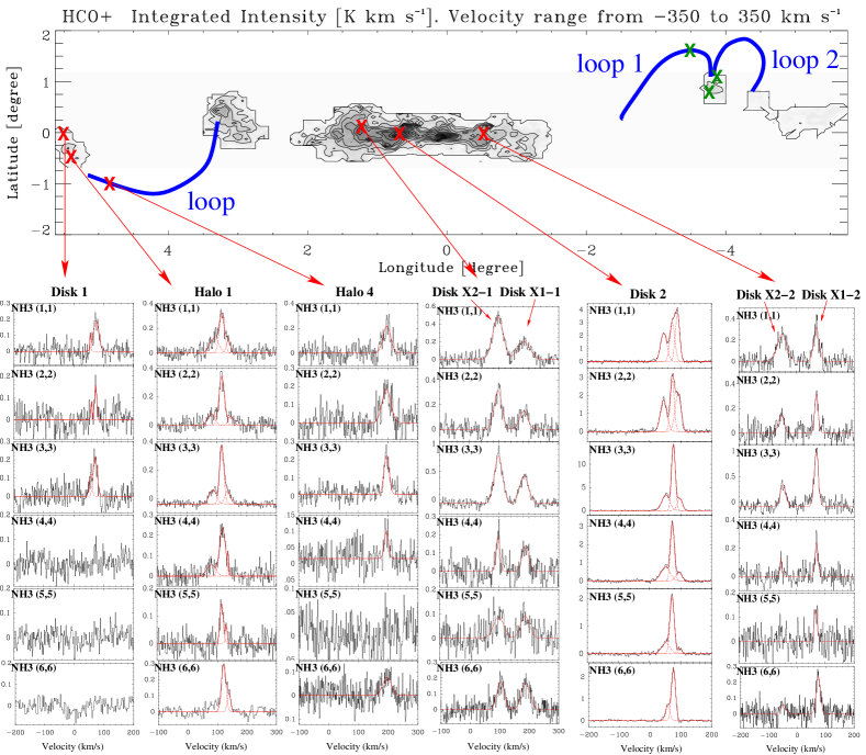
Figure 1: Spectra toward selected positions in the GC in the metastable inversion transitions from (1,1) to (6,6) of NH₃. The positions are indicated in the HCO⁺ integrated intensity map from Riquelme et al. (2010b). The GMLs found by Fukui et al. (2006) are indicated in blue. The positions which could not seen from Effelsberg are indicated with green crosses. As indicated in Table 1, our Disk 2 position corresponds to Sgr B2.

3 Results

Fig. 1 shows the ammonia spectra taken toward each position in all the metastable inversion transitions observed in this work. Most of the metastable inversion transitions of NH₃ were detected, except the (4,4), (5,5), and (6,6) of “Disk 1” and the (5,5) of “Halo 4”. The criteria used to define if a emission line is detected or not, was to have a line peak temperature $>3\sigma_{\mathrm{rms}}$, where $\sigma_{\mathrm{rms}}$ is the root mean square per spectral channel. If the intensity of the line does not reach this value, we still assume that a line is actually detected if the line has an integrated intensity in the velocity width (as defined by the (3,3) line which presents the highest signal-to-noise ratio) $>3\sigma$.

3.1 Optical depth of NH₃

Each NH₃ inversion transition is split into five components: a “main component” and four symmetrically placed “satellites” (the quadrupole hyperfine (HF) structure). Due to the large linewidth of the molecular clouds in the GC, the magnetic splitting ($<0.2{{\rm\;km\;s^{-1}}}$) cannot be resolved. Under the assumption of local thermodynamical equilibrium (LTE), the relative intensities of the four satellite HF components can be used to estimate the optical depth $\tau$ of the main component of the metastable inversion transitions. Knowing $\tau$, we can estimate the NH₃ column density, and the rotational temperature from the ratios of the peak or integrated intensities.
We use the “NH₃ method” from CLASS to determine the optical depth for the $(1,1)$, $(2,2)$ and $(3,3)$ lines. To define the linewidth (which was used as a fixed parameter in the NH₃ method), we use the $(3,3)$ transition, because these spectra have the best signal-to-noise ratio in our observations and the HF components are much weaker than those of the $(1,1)$ and $(2,2)$ lines. As we can see in Table LABEL:observation, all the NH₃ lines observed in this work are optically thin toward all sources, except the $(1,1)$ transition toward Sgr B2. Following the criteria of Hüttemeister et al. (1993a) based on the lower peak intensities in these lines, with respect to the $(1,1)$, $(2,2)$ and $(3,3)$ ones, we assume that the $(4,4)$ and $(5,5)$ are also optically thin. Table LABEL:observation presents the results from simple Gaussian fits for all the observed positions, allowing all the parameters to be free.

3.2 Physical conditions of the gas from CS and NH₃

To derive the $n(\mathrm{H_{2}})$ and $T_{\mathrm{kin}}$ of the gas, we combine the CS and NH₃ molecular emission, in an iterative way. First, we used MASSA software to derive the rotational temperatures and column densities using Boltzmann diagrams (see, Goldsmith & Langer 1999, for a detailed explanation and equations of the method) (Table 2). The rotational temperature, which is a lower limit of the actual kinetic temperature, $T_{\mathrm{kin}}$, was used as a fixed parameter in RADEX (see, van der Tak et al. 2007, for detailed explanation of the formalism adopted in this statistical equilibrium radiative transfer code) to derive the $n(\mathrm{H_{2}})$ and CS column densities. Then, using the $n(\mathrm{H_{2}})$ obtained from CS, we used RADEX to derive the kinetic temperature from the para-NH₃ transitions (see §3.2.2). With the kinetic temperature, we derived then the final $n(\mathrm{H_{2}})$ and CS column densities (Table 3).

Table 2: NH₃ physical parameters (rotational temperatures and column densities) derived for each source using MASSA software. Bold faced values indicated the most likely result consistent with the non-LTE analysis.

Source	$n^{a}$	$T_{\rm rot}$	$T_{\rm rot}$	$T_{\rm rot}$	$T_{\rm rot}$	$N({\rm NH_{3}})$	$N({\rm NH_{3}})$	$N({\rm NH_{3}})$	$N($o-NH${}_{3})$
		(11-22)	(22-44-55)	(11-22-44-55)	(33-66)	(11-22)	(22-44-55)	(11-22-44-55)	(33-66)
		[K]	[K]	[K]	[K]	1014 cm-2	1014 cm-2	1014 cm-2	1014 cm-2
Halo1	1	$46.7\pm 0.9$	$117.5\pm 1.7$	${\bf 92.7\pm 0.8}$	$81.0\pm 0.8$	$2.14\pm 0.07$	$3.53\pm 0.10$	${\bf 3.72\pm 0.06}$	$5.37\pm 1.1$
	2	$43.2\pm 0.3$	$131.8\pm 0.9$	${\bf 96.6\pm 0.3}$	$156.4\pm 9.6$	$4.93\pm 0.06$	$9.09\pm 0.11$	${\bf 9.49\pm 0.06}$	$11.1\pm 1.2$
	3			$80.9\pm 1.1$	$169\pm 31$			$2.06\pm 0.06$	$3.3\pm 1.0$
Halo4	1			$56.5\pm 2.3$	$138\pm 10$			$5.48\pm 0.45$	$5.39\pm 0.76$
DiskX1-1	1	$27.2\pm 1.5$	$156\pm 12$		$164.1\pm 6.6$	$4.85\pm 0.53$	$7.7\pm 1.2$		$12.07\pm 0.91$
DiskX2-1	1	$27.4\pm 0.8$	$91.7\pm 3.6$		$122.8\pm 3.8$	$9.75\pm 0.52$	$9.87\pm 0.78$		$16.56\pm 0.98$
DiskX1-2	1	$33.1\pm 2.2$	$112.7\pm 6.5$		$138.2\pm 5.1$	$3.99\pm 0.48$	$5.75\pm 0.71$		$10.93\pm 0.80$
DiskX2-2	1	$22.0\pm 1.4$	$72.5\pm 6.1$		$106.9\pm 9.7$	$4.44\pm 0.55$	$2.85\pm 0.58$		$5.09\pm 0.90$
Disk1	1	$19.1\pm 2.9$	$154\pm 48$		$139\pm 26$	$0.74\pm 0.20$	$0.66\pm 0.41$		$0.93\pm 0.39$
	2	$26.9\pm 2.4$	$82.9\pm 9.8$		$100\pm 12$	$1.41\pm 0.20$	$1.29\pm 0.34$		$2.02\pm 0.46$
Disk2	1	${\bf 38.1\pm 0.6}$	${\bf 110.3\pm 1.0}$	$90.6\pm 0.5$	$95.7\pm 1.5$	${\bf 31.6\pm 1.0}$	${\bf 48.1\pm 1.1}$	$60.3\pm 1.0$	$61.0\pm 2.0$
	2	$50.8\pm 1.6$	$145.6\pm 2.3$	${\bf 113.8\pm 0.5}$	$112.9\pm 0.6$	$42.1\pm 2.1$	$84.9\pm 3.1$	${\bf 101.6\pm 1.0}$	$133.2\pm 1.4$
	3	${\bf 33.0\pm 0.9}$	${\bf 63.1\pm 1.2}$	$51.7\pm 0.5$	$52.4\pm 3.2$	${\bf 33.1\pm 1.3}$	${\bf 32.0\pm 1.7}$	$47.2\pm 1.0$	$37.6\pm 6.4$

• ^a Cloud number defined by the different velocity components (see Table LABEL:observation)

• $N(para-{\rm NH_{3}}$) correspond to the sum of all observed para-NH₃ column densities. When the data is consistent with a two temperature model, $N(para-{\rm NH_{3}})$ correspond to the sum of column 7 and 8. If only one temperature regime is present, the $N(para-{\rm NH_{3}})$ corresponds to column 9.

3.2.1 $n(\mathrm{H_{2}})$ derived from the CS data

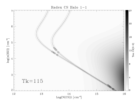
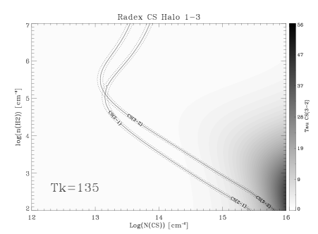
Figure 12: LVG diagrams of CS for each velocity component (defined by the J=2-1 CS) of Halo 1 (see Table LABEL:SiO-CS-HNCO) . Top: 83.8 km s^-1. Middle: $117.4\,{\rm km\,s}^{-1}$. Bottom: $136.9\,{\rm km\,s}^{-1}$. The $T_{{\rm kin}}$ is indicated in the lower left corner in each plot.

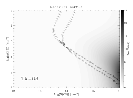
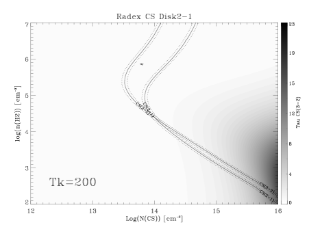
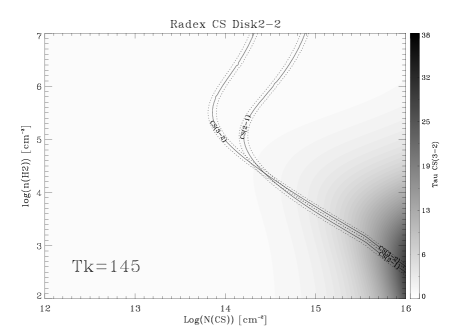
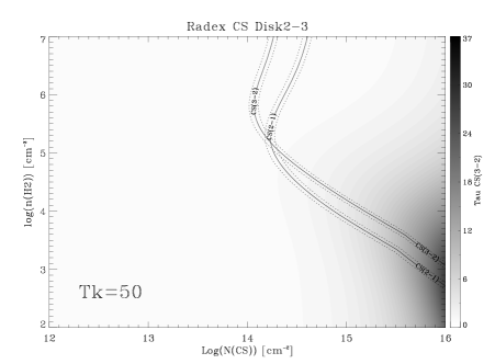
Figure 22: LVG diagrams of CS for each kinetic temperature regime, for each velocity component of Disk 2. Top: $14.2\,{\rm km\,s}^{-1}$. Middle: $55.9\,{\rm km\,s}^{-1}$. Bottom: $79.0\,{\rm km\,s}^{-1}$.

We used the non-LTE excitation radiative transfer code RADEX to derive the $n(\mathrm{H_{2}})$ and CS column densities from line intensities of the observed CS lines. The modeling suggests that the CS emission is optically thin with opacities ranging from 0.05 to 0.96. The results are showed in Table 3. The error were estimated assuming a 10% calibration error as the typical flux calibration uncertainty at the 30-m telescope, and we give an upper and lower value based on the minimum and maximum value from the LVG diagrams (see from Fig. 12 to Fig. 22). It is important to note that $n(\mathrm{H_{2}})$ in some sources is poorly constrained, which translates in large errors or upper limits shown in the Table 4. If we derive the $n(\mathrm{H_{2}})$ using the rotational temperature (which is a lower limit to the kinetic temperature), the $n(\mathrm{H_{2}})$ differ on average by $\sim 27$%.

Table 3: Physical parameters derived from CS using non-LTE (RADEX) model. The kinetic temperature used in RADEX is indicated. When more than one $T_{{\rm kin}}$ regime was present in one position, we derived the physical parameters from each $T_{{\rm kin}}$. We assumed a 10% calibration error.

Source	Cloud	$T_{kin}$	Tex CS(2-1)	Tex CS(3-2)	$\tau_{CS(2-1)}$	$\tau_{CS(3-2)}$
	number	[K]	[K]	[K]
Halo1	1	$115$	$<3.8$	$<3.6$	$>0.25$	$>0.16$
	2	$90$	$12.6^{9.3}_{4.3}$	$8.2^{2.5}_{1.8}$	$0.25^{0.35}_{0.15}$	$0.54^{0.34}_{0.18}$
	3	$135$	$4.6^{1.7}_{1.1}$	$4.4^{1.0}_{0.9}$	$0.31^{1.06}_{0.18}$	$0.35^{0.77}_{0.14}$
Halo2	1	$113$	$4.1^{1.3}_{0.8}$	$4.0^{0.9}_{0.8}$	$0.22^{0.75}_{0.13}$	$0.14^{0.31}_{0.06}$
	2	$113$	$3.8^{1.3}_{0.8}$	$3.8^{0.9}_{0.9}$	$0.28^{15.3}_{0.18}$	$0.15^{5.81}_{0.07}$
Halo3	1	$113$	$4.7^{1.8}_{0.0}$	$4.4^{1.1}_{0.0}$	$0.61^{0.10}_{0.38}$	$0.75^{0.12}_{0.35}$
	2	$113$	$6.1^{3.1}_{1.7}$	$5.2^{1.2}_{1.0}$	$0.07^{0.11}_{0.04}$	$0.05^{0.04}_{0.02}$
Halo4	1	$95$	$5.4^{2.3}_{1.2}$	$4.7^{1.1}_{0.8}$	$0.21^{0.28}_{0.12}$	$0.17^{0.12}_{0.06}$
Halo5	1	$95$	$10.4^{8.4}_{3.4}$	$7.0^{2.2}_{1.4}$	$0.11^{0.13}_{0.07}$	$0.21^{0.10}_{0.07}$
Disk-X1-1	1	$38$	$10.9^{5.6}_{3.1}$	$7.1^{1.9}_{1.2}$	$0.12^{0.10}_{0.06}$	$0.24^{0.09}_{0.07}$
		$300$	$9.3^{8.3}_{3.0}$	$6.8^{2.2}_{1.4}$	$0.15^{0.20}_{0.09}$	$0.25^{0.14}_{0.09}$
Disk-X2-1	1	$38$	$6.7^{2.4}_{1.6}$	$5.3^{1.1}_{0.9}$	$0.37^{0.51}_{0.19}$	$0.48^{0.37}_{0.15}$
		$100$	$5.9^{2.5}_{1.4}$	$5.0^{1.3}_{1.1}$	$0.50^{1.23}_{0.29}$	$0.55^{0.85}_{0.22}$
Disk-X1-2	1	$52$	$13.7^{8.4}_{4.4}$	$8.5^{2.4}_{1.7}$	$0.16^{0.16}_{0.08}$	$0.42^{0.18}_{0.13}$
		$215$	$12.9^{15.5}_{4.7}$	$8.4^{2.9}_{1.8}$	$0.18^{0.24}_{0.12}$	$0.43^{0.23}_{0.15}$
Disk-X2-2	1	$28$	$10.0^{3.8}_{2.5}$	$6.7^{1.6}_{1.2}$	$0.20^{0.18}_{0.09}$	$0.30^{0.13}_{0.08}$
		$95$	$9.3^{7.1}_{2.8}$	$6.6^{2.1}_{1.3}$	$0.22^{0.28}_{0.14}$	$0.31^{0.17}_{0.11}$
Disk1	1	$23$	$<3.4$	$<3.3$	$>0.22$	$>0.14$
		$154$	$<3.0$	$<3.0$	$>0.57$	$>0.30$
	2	$38$	$5.5^{2.1}_{1.2}$	$4.7^{1.0}_{0.7}$	$0.17^{0.20}_{0.09}$	$0.17^{0.10}_{0.05}$
		$82$	$5.0^{1.9}_{1.1}$	$4.5^{1.0}_{0.8}$	$0.21^{0.37}_{0.12}$	$0.19^{0.18}_{0.07}$
Disk2	1	$68$	$6.8^{3.5}_{1.7}$	$5.4^{1.4}_{0.9}$	$0.16^{0.19}_{0.09}$	$0.21^{0.12}_{0.07}$
		$200$	$6.1^{2.9}_{1.6}$	$5.3^{1.3}_{1.0}$	$0.20^{0.28}_{0.11}$	$0.23^{0.17}_{0.08}$
	2	$145$	$6.7^{2.9}_{1.7}$	$5.7^{1.4}_{1.2}$	$0.70^{14.8}_{0.41}$	$0.96^{15.2}_{0.40}$
	3	$50$	$16.1^{9.2}_{5.6}$	$9.4^{2.7}_{2.1}$	$0.19^{0.22}_{0.09}$	$0.45^{0.23}_{0.13}$
		$80$	$16.1^{16.2}_{6.2}$	$9.3^{3.5}_{2.2}$	$0.19^{0.27}_{0.12}$	$0.45^{0.26}_{0.16}$

3.2.2 LVG analysis from NH₃

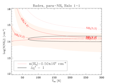
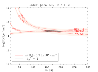
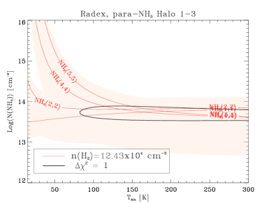
Figure 4: LVG diagrams of NH₃ for each velocity component of Halo 1. Top: $87.7\,{\rm km\,s}^{-1}$ . Middle: $117.2\,{\rm km\,s}^{-1}$. Bottom: $138.6\,{\rm km\,s}^{-1}$.

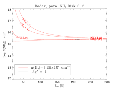
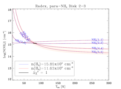
Figure 11: LVG diagrams of NH₃ for each velocity component of Disk 2. Top: $48.8\,{\rm km\,s}^{-1}$. Middle: $74.5\,{\rm km\,s}^{-1}$. Bottom: $95.8\,{\rm km\,s}^{-1}$. The blue lines correspond to the low temperature regimen, and the red lines to the high temperature regimen.

To estimate the kinetic temperatures of the gas, we also used a non-LTE excitation and radiative transfer code RADEX. Using the value of $n(\mathrm{H_{2}})$ derived from the CS LVG analysis (Table 4), and the velocity widths (see Table LABEL:observation), we can derive the $T_{\rm kin}$ and $N_{{\rm NH_{3}}}$. Fig. 2 shows an example of this procedure, and Table 4 shows the results. In Fig. 2 and from Fig. 4 to Fig. 11, we show in blue the results corresponding to the metastable inversion transitions $(1,1)$-$(2,2)$ (low rotational temperature), and in red, the results corresponding to the metastable inversion transitions $(2,2)$-$(4,4)$-$(5,5)$ (high rotational temperature). For the cases where only one temperature regimen was a possible solution, we plotted the result in red in the LVG plot. LVG models indicate that the results from LTE are reliable. Additionally, for every observed position, we checked the two temperature component assumption by comparison to synthetic spectra under LTE approach using MASSA software. We found that for the positions where we derived two kinetic temperature components, the modeled line profile fit better the observed emission, while a single warm component was not enough to reproduce the observed profile. When the $(4,4)$ or $(5,5)$ inversion transitions were not detected, the upper limits to their emission were plotted in dashed lines. This upper limit to the emission was obtained as 3$\sigma_{\mathrm{rms}}$ level. The individual fits to all sources are shown in the Online Appendix (Fig.4 to 11).

As a result of our analysis, we derive two kinetic temperature (one cool and one warm) components in the CMZ and only one warm component in the halo positions. In the CMZ the cool component range from $23$ K to $68$ K with an average value of $40$ K; and the warm component range from $80$ K to $>300$ K with an average value of $150$ K. This reference values should be taken with caution due to the large uncertainty of the kinetic temperature derived from the LVG (see below). To estimate the uncertainty of the derived parameters, we computed the $\chi^{2}$ of the line intensities over the grid used for the LVG model. We impose $\Delta\chi^{2}=\chi^{2}-\chi^{2}_{\mathrm{min}}=1$, which translates in the $68.3$% confidence level projected for each parameter axis (see, e.g., Press et al. 1992, Section §15.6). The black ellipses shows the error in the model (Fig. 2).

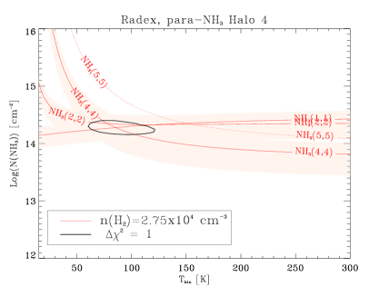
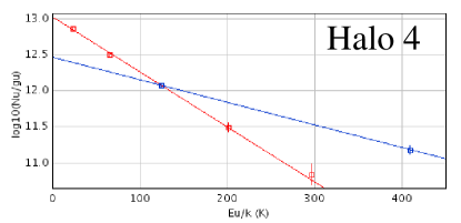
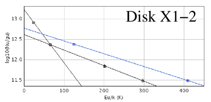
Figure 2: Example of rotational (bottom) and LVG (top) diagrams of NH₃. Left: Halo 4. Right: Disk X1-2. In the Boltzmann diagram (bottom), para-NH₃ species are fitted with the red line, and the ortho-NH₃ species are fitted with the blue line. In the LVG diagrams (top), we plot the peak intensity of the metastable inversion transitions of para-NH₃. For the source Halo 4, we derive only one kinetic temperature component (warm), which is plotted in red lines, and the error in red shaded region. The source Disk X1-2 was modeled using two kinetic temperature component model, one warm and one cold, that were plotted in red and blue lines respectively with the correspondly associated error shown as shaded regions. We show the $n(\mathrm{H_{2}})$ used in the LVG model for the warm and cold components. To estimate the uncertainty of the derived parameters, we computed the $\chi^{2}$ of the line intensities over the grid used for the LVG model. We impose $\Delta\chi^{2}=\chi^{2}-\chi^{2}_{\mathrm{min}}=1$, which translates in the $68.3$% (1 $\sigma$) confidence level projected for each parameter axis

(see text for details).

Table 4: Kinetic temperatures and densities derived from LVG calculations from NH₃ and CS data

Source	Cloud	low temperature		high temperature		single temperature from p$-$NH3
	number	$T_{{\rm kin}}$	$n({\rm H_{2}})$	$T_{{\rm kin}}$	$n({\rm H_{2}})$	$T_{{\rm kin}}$	$n({\rm H_{2}})$
		[K]	104 cm-3	[K]	104 cm-3	[K]	104 cm-3
Halo1	1					$>115$	$<1.00$
	2					$>90$	$8.49^{5.63}_{4.08}$
	3					$>135$	$1.58^{1.72}_{1.23}$
Halo2	1					$113^{c}$	$1.26^{1.56}_{0.98}$
	2					$113^{c}$	$<2.51$
Halo3	1					$113^{c}$	$1.50^{2.05}_{0.09}$
	2					$113^{c}$	$3.55^{2.76}_{1.96}$
Halo4	1					$95$	$2.75^{2.54}_{1.49}$
Halo5	1					$95^{c}$	$7.47^{5.11}_{3.18}$
DiskX1-1	1	$38$	$13.0^{8.21}_{5.05}$	$>300^{a}$	$3.55^{2.56}_{1.66}$
DiskX2-1	1	$38$	$5.62^{4.38}_{3.11}$	$100$	$2.70^{2.73}_{1.90}$
DiskX1-2	1	$52$	$13.3^{8.09}_{5.34}$	$215$	$5.62^{3.88}_{2.46}$
DiskX2-2	1	$28$	$14.1^{8.88}_{5.98}$	$95$	$6.20^{5.02}_{2.95}$
Disk1	1	$23$	$<1.12$	$>154^{b}$	$<0.16$
	2	$38$	$4.57^{3.84}_{2.33}$	$>82^{b}$	$2.51^{2.40}_{1.55}$
Disk2	1	$68$	$4.97^{3.94}_{2.40}$	$200$	$2.47^{2.00}_{1.35}$
	2					$>145$	$2.51^{2.50}_{2.41}$
	3	$50$	$15.8^{9.27}_{6.94}$	$80$	$11.6^{8.32}_{5.32}$

• ^a LVG gives a $T_{{\rm kin}}$ greater than 300 K which is the value allowed by the collisional rates given by Danby et al. (1988).

• ^b Due that the values for the (4,4)-(5,5) metastable inversion transitions are upper limits to the actual $T_{\rm MB}$, the modeled curve in the LVG plot is outside the allowed range, and we give a lower limit to the kinetic temperature using the rotational temperature form the LTE plot.

• ^c The assumed value for the kinetic temperature for positions were there are no NH₃ observations is the average of the $T_{{\rm kin}}$ from similar positions.

3.3 Column densities and relative abundances from other molecules

To shed light on the physical processes that are heating the molecular gas, we derived also relative abundances of NH₃ with respect to the following molecules: SiO, which is a well-known shock tracer (Martín-Pintado et al. 1992), CS which is a high-density gas tracer ($n>10^{4}{\rm cm}^{-3}$ Mauersberger & Henkel 1989; Mauersberger et al. 1989), and HNCO which is a tracer of shocks, and very high densities, ($n_{{\rm H_{2}}}\geq 10^{6}{\rm cm}^{-3}$, Jackson et al. 1984; Martín et al. 2008; Zinchenko et al. 2000) with a high photodissociation rate (Table 8). We also derive the fractional abundances of these molecules with respect to H₂ as traced by ¹³CO (Table 6). We assumed that they arise from the same volume. This assumption may not be fulfilled for all of our observed position due to the observed differences in the velocity center and linewidth (see Table LABEL:SiO-CS-HNCO). In all the calculations we assume that the GC sources are extended, therefore we take $T_{\rm B}\sim T_{\rm MB}$.

3.3.1 Column densities of SiO, HNCO, ¹³CO, and C¹⁸O

We used the non-LTE excitation radiative transfer code RADEX to derive the column densities. For the species with only one observed transition (SiO, HNCO, and CO isotopes), we are forced to make some assumptions about the physical properties of the gas ($T_{\mathrm{kin}}$ and $n(\mathrm{H_{2}})$). We used the kinetic temperatures derived by NH₃, and the $n(\mathrm{H_{2}})$ from the CS data (Table 4). The results are shown in Table 5. The column densities agree within a factor of 3-4 if we use the LTE approach (Table LABEL:SiO-CS-HNCO) for a $T_{\mathrm{ex}}=10$ K (which is consistent with the value derived for SiO by Hüttemeister et al. (1998), and with our $T_{\mathrm{ex}}$ value derived from CS shown in Table 3).

Using $n(\mathrm{H_{2}})\sim 10^{3}$ cm^-3 (because the critical density of CO is lower than for CS) the column densities for the CO isotopes are a factor 2-4 lower than using the $n(\mathrm{H_{2}})\sim 10^{4}$ cm^-3.

Table 5: Column densities from different molecules derived from RADEX using as a fixed parameter the kinetic temperatures and the $n(\mathrm{H_{2}})$ (Table 4)

Source	Cloud	Tkin	N(p-NH3)	N(CS)	N(SiO)	N(HNCO)	N(C34S)	N(13CO)	N(C18O)	N(H2)a
	number	[K]	[$10^{14}\rm{cm}^{-2}$]	[$10^{13}\rm{cm}^{-2}$]	[$10^{13}\rm{cm}^{-2}$]	[$10^{13}\rm{cm}^{-2}$]	[$10^{13}\rm{cm}^{-2}$]	[$10^{16}\rm{cm}^{-2}$]	[$10^{16}\rm{cm}^{-2}$]	[$10^{21}\rm{cm}^{-2}$]
Halo1	1	$115$	$1.07^{0.68}_{0.27}$	$>6.73$	$>2.24$	$>0.50$	$-$	$4.47^{0.52}_{3.47}$	$0.52^{0.07}_{0.41}$	$23.53^{2.74}_{18.26}$
	2	$90$	$2.24^{0.11}_{0.26}$	$15.99^{6.50}_{2.56}$	$4.35^{1.96}_{0.87}$	$2.89^{0.79}_{0.46}$	$1.20^{0.44}_{0.17}$	$4.03^{0.67}_{0.75}$	$0.97^{0.17}_{0.18}$	$21.21^{3.53}_{3.95}$
	3	$135$	$0.70^{0.15}_{0.34}$	$6.53^{17.17}_{2.74}$	$1.88^{5.20}_{0.86}$	$-$	$-$	$2.00^{0.75}_{1.06}$	$0.16^{0.08}_{0.09}$	$10.53^{3.95}_{5.58}$
Halo2	1	$113$	$-$	$5.75^{16.65}_{2.73}$	$0.76^{2.45}_{0.38}$	$1.64^{4.83}_{0.75}$	$0.33^{1.67}_{0.21}$	$-$	$-$	$-$
	2	$113$	$-$	$>2.91$	$>0.34$	$-$	$>0.13$	$-$	$-$	$-$
Halo3	1	$113$	$-$	$22.52^{3.55}_{10.64}$	$3.98^{0.59}_{1.99}$	$4.47^{0.55}_{1.74}$	$1.43^{0.36}_{0.70}$	$-$	$-$	$-$
	2	$113$	$-$	$3.71^{3.05}_{1.07}$	$-$	$1.27^{0.72}_{0.19}$	$0.29^{0.34}_{0.13}$	$-$	$-$	$-$
Halo4	1	$95$	$1.99^{0.53}_{0.56}$	$6.18^{5.32}_{2.17}$	$1.00^{1.00}_{0.38}$	$3.98^{2.69}_{0.80}$	$0.40^{0.42}_{0.18}$	$7.35^{1.83}_{2.07}$	$0.25^{0.08}_{0.08}$	$38.68^{9.63}_{10.89}$
Halo5	1	$95$	$-$	$5.29^{1.83}_{0.93}$	$0.99^{0.42}_{0.22}$	$2.58^{0.76}_{0.32}$	$0.47^{0.14}_{0.08}$	$-$	$-$	$-$
Disk-X1-1	1	$38$	$1.99^{0.67}_{0.56}$	$12.64^{3.33}_{1.91}$	$3.91^{1.30}_{0.76}$	$3.05^{0.74}_{0.48}$	$0.64^{0.20}_{0.12}$	$8.84^{1.12}_{1.15}$	$0.51^{0.19}_{0.18}$	$46.53^{5.89}_{6.05}$
		$300$	$1.58^{0.58}_{0.48}$	$13.78^{6.31}_{2.82}$	$3.98^{2.00}_{0.90}$	$2.88^{0.67}_{0.33}$	$0.71^{0.35}_{0.18}$	$32.8^{9.39}_{8.73}$	$1.87^{1.08}_{0.87}$	$172.63^{49.42}_{45.95}$
Disk-X2-1	1	$38$	$4.47^{0.39}_{0.69}$	$19.07^{15.10}_{5.44}$	$3.36^{2.95}_{1.12}$	$9.59^{4.00}_{1.02}$	$0.80^{0.64}_{0.24}$	$16.9^{2.45}_{2.94}$	$1.37^{0.23}_{0.27}$	$33.80^{4.90}_{5.88}$
		$100$	$3.30^{0.43}_{0.98}$	$22.56^{37.65}_{8.27}$	$3.60^{6.76}_{1.36}$	$10.6^{13.0}_{2.01}$	$0.98^{1.60}_{0.37}$	$29.2^{7.55}_{11.1}$	$2.51^{0.77}_{0.98}$	$58.40^{15.10}_{22.20}$
Disk-X1-2	1	$52$	$1.66^{0.27}_{0.31}$	$10.60^{2.63}_{1.28}$	$2.09^{0.62}_{0.35}$	$3.19^{0.89}_{0.56}$	$0.71^{0.15}_{0.09}$	$3.10^{0.40}_{0.41}$	$0.32^{0.05}_{0.05}$	$16.32^{2.11}_{2.16}$
		$215$	$1.51^{0.30}_{0.33}$	$11.03^{3.71}_{1.70}$	$2.10^{0.78}_{0.37}$	$2.96^{0.96}_{0.39}$	$0.74^{0.22}_{0.11}$	$8.09^{1.81}_{1.78}$	$0.82^{0.23}_{0.21}$	$42.58^{9.53}_{9.37}$
Disk-X2-2	1	$28$	$1.90^{0.51}_{0.55}$	$10.67^{3.49}_{1.73}$	$0.22^{0.07}_{0.04}$	$2.08^{0.42}_{0.32}$	$0.93^{0.29}_{0.15}$	$12.8^{1.55}_{1.58}$	$1.14^{0.13}_{0.14}$	$25.60^{3.10}_{3.16}$
		$95$	$1.00^{0.60}_{0.52}$	$11.07^{5.26}_{2.48}$	$0.27^{0.19}_{0.08}$	$2.00^{0.57}_{0.25}$	$0.96^{0.48}_{0.19}$	$28.7^{5.26}_{5.83}$	$2.62^{0.52}_{0.53}$	$57.40^{10.52}_{11.66}$
Disk1	1	$23$	$0.40^{1.84}_{0.26}$	$>2.90$	$>0.25$	$>1.12$	$>0.03$	$1.26^{0.52}_{0.55}$	$0.13^{0.05}_{0.07}$	$2.52^{1.04}_{1.10}$
		$154$	$>0.16$	$>7.20$	$>1.43$	$>2.82$	$>0.09$	$1.32^{0.15}_{0.61}$	$0.14^{0.02}_{0.08}$	$2.64^{0.30}_{1.22}$
	2	$38$	$0.63^{0.20}_{0.19}$	$3.89^{2.80}_{1.25}$	$0.45^{0.37}_{0.17}$	$1.72^{0.79}_{0.27}$	$0.16^{0.13}_{0.06}$	$2.26^{0.35}_{0.40}$	$0.19^{0.04}_{0.04}$	$4.52^{0.70}_{0.80}$
		$82$	$>0.45$	$4.54^{5.48}_{1.70}$	$0.50^{0.62}_{0.22}$	$2.00^{1.99}_{0.52}$	$0.19^{0.26}_{0.08}$	$3.46^{0.85}_{1.08}$	$0.28^{0.09}_{0.10}$	$6.92^{1.70}_{2.16}$
Disk2	1	$68$	$14.1^{0.19}_{0.15}$	$8.98^{5.18}_{2.46}$	$2.98^{2.12}_{0.87}$	$-$	$3.05^{1.83}_{0.76}$	$-$	$-$	$-$
		$200$	$14.1^{0.02}_{0.16}$	$10.03^{8.07}_{3.04}$	$3.16^{2.71}_{1.06}$	$-$	$3.45^{2.86}_{1.04}$	$-$	$-$	$-$
	2	$145$	$25.1^{0.07}_{0.07}$	$>16.51$	$>5.63$	$>264.4$	$>5.67$	$101.28^{28.47}_{78.30}$	$19.63^{6.48}_{16.39}$	$202.56^{56.94}_{156.60}$
	3	$50$	$14.1^{0.09}_{0.05}$	$16.89^{4.31}_{1.86}$	$-$	$-$	$-$	$-$	$-$	$-$
		$80$	$12.1^{0.07}_{0.07}$	$17.05^{5.18}_{2.08}$	$-$	$-$	$-$	$-$	$-$	$-$

• ^a Column densities of H₂ derived from ¹³CO using a conversion factor of $5.0\times 10^{-6}$ (Rodríguez-Fernández et al. 2001) for the normal GC gas, and a factor of $1.9\times 10^{-6}$ for the gas in the disk-halo interaction regions (see text for details).

The total column density of H₂ can be estimated from the CO isotopologues, that have lower optical depths than the main isotope, and therefore a more reliable estimation of the column density ($N({\rm H_{2}})=N({\rm{}^{x}C^{y}O})\times[{\rm{}^{x}C^{y}O/H_{2}}]$, where $x$ and $y$ correspond to the isotopic substitution used for the carbon and oxygen atoms). For our calculations, we assume an abundance ratio CO/H₂ of 10^-4 (see, e.g., Rodríguez-Fernández et al. 2001, and references therein), and we use the ¹³CO emission. Therefore, we also need the ¹²C/¹³C isotopic ratio. Recently, Riquelme et al. (2010a) derived a high ¹²C/¹³C isotopic value ($>40$) in some of the sources studied in this work. Such a high isotopic value was found mainly toward the disk-halo interaction regions, therefore, we still use the standard value of 20 (see, e.g., Wilson & Matteucci 1992) in the typical GC gas for the sources “Disk1”, “Disk2” and for the sources with kinematic of X2 orbits (Disk X2-1, Disk X2-2). For the sources which are in the disk-halo interaction regions, we used the value of 53 corresponding to the typical value found in the 4 kpc molecular ring (Wilson & Rood 1994), which also was used by Torii et al. (2010a) and Kudo et al. (2011) in the GMLs regions. This translates in using a $\mathrm{[^{13}CO/H_{2}]}$ conversion factor of $5.0\times 10^{-6}$ for the normal GC gas, and $1.9\times 10^{-6}$ for the gas in the disk-halo interaction regions (Table 5). We decided not to use the C¹⁸O emission to trace the total column density of H₂, because of the uncertainties in the ¹⁶O/¹⁸O isotopic ratio in the disk-halo interaction regions, which could be affected by the unprocessed gas that is being accreted toward the GC region (Riquelme et al. 2010a).

3.3.2 Fractional abundances

We derived beam averaged fractional abundances with respect to H₂ for all the observed molecules (Table 6), and in Table 8 we show the results of the fractional abundances of NH₃ with respect to the other molecules, and the fractional abundances of SiO and HNCO with respect to CS and C³⁴S.

Table 6: Fractional abundances of SiO, HNCO, NH₃, CS, and C³⁴S with respect to H₂

Source	$n^{a}$	$X({\rm SiO})$	$X({\rm HNCO})$	$X({\rm NH_{3}})^{b}$	$X({\rm CS})$	$X({\rm C^{34}S})$
		$\times 10^{-9}$	$\times 10^{-9}$	$\times 10^{-8}$	$\times 10^{-9}$	$\times 10^{-10}$
Halo1	1	$1.42\pm 0.95$	$0.32\pm 0.21$	$1.70\pm 1.25$	$4.27\pm 2.84$
	2	$2.33\pm 0.79$	$1.45\pm 0.39$	$2.12\pm 0.40$	$9.16\pm 2.25$	$6.36\pm 1.84$
	3	$4.17\pm 3.73$		$1.42\pm 0.77$	$14.15\pm 12.38$
Halo2	1
	2
Halo3	1
	2
Halo4	1	$0.34\pm 0.20$	$1.29\pm 0.58$	$1.11\pm 0.37$	$2.04\pm 1.13$	$1.37\pm 0.87$
Halo5	1
DiskX1-1	1	$0.39\pm 0.12$	$0.28\pm 0.07$	$0.35\pm 0.09$	$1.31\pm 0.37$	$0.67\pm 0.20$
DiskX2-1	1	$1.20\pm 0.58$	$3.08\pm 1.12$	$1.72\pm 0.41$	$6.94\pm 3.24$	$2.94\pm 1.39$
DiskX1-2	1	$0.77\pm 0.18$	$1.12\pm 0.25$	$1.10\pm 0.21$	$3.95\pm 0.86$	$2.60\pm 0.54$
DiskX2-2	1	$0.07\pm 0.02$	$0.52\pm 0.10$	$0.76\pm 0.18$	$2.91\pm 0.70$	$2.55\pm 0.60$
Disk1	1	$3.60\pm 1.01$	$8.44\pm 2.37$	$2.40\pm 0.67$	$21.63\pm 6.08$	$2.57\pm 0.72$
	2	$1.12\pm 0.49$	$4.22\pm 1.45$	$1.94\pm 0.36$	$9.94\pm 4.13$	$4.21\pm 1.87$
Disk2	1
	2	$0.37\pm 0.26$	$17.31\pm 12.10$	$3.29\pm 2.30$	$1.08\pm 0.76$	$3.71\pm 2.60$
	3

• ^a Cloud number defined by the different velocity components.

• ^b Column density of NH₃ correspond to the $N(p-NH_{3})+N(o-NH_{3})=2\times N(p-NH_{3})$ assuming a ortho-to-para ratio of 1.

The results for Disk 1, will be disscused below. $X({\rm SiO})$ varies from $0.07-4.17\times 10^{-9}$ with the largest value toward the foot points of the GMLs. $X({\rm HNCO})$ shows less variation in all the observed sources ranging from $0.28$ to $3.08\times 10^{-9}$, except for the Disk 2, which has a large abundance of $17.31\times 10^{-9}$. The fractional abundances with respect to H₂ depend on a reliable estimation of the H₂ column density, which depends in a number of assumption (H₂ to CO conversion factor, physical parameters used to derive the column densities of ¹³CO). Therefore, we also compare the column density of the different molecular tracer (shock, photodissociation) with respect to CS (dense tracer) and its C³⁴S isotope (Table 8), which is almost certainly optically thin because in the GC region ³⁴S is $\sim 10$ times rarer than the main isotope (Chin et al. 1996).

Although there are no big differences from source to source in the $N(\mathrm{SiO})/N(\mathrm{CS})$ and $N(\mathrm{SiO})/N(\mathrm{C^{34}S})$ ratios, we can see that the highest values are found toward Halo 1 and Disk X1 sources, with a difference up to 1 order of magnitude if we compare the Disk X1-2 with the Disk X2-2 sources. The relative abundance $N(\mathrm{HNCO})/N(\mathrm{CS})$ and $N(\mathrm{HNCO})/N(\mathrm{C^{34}S})$ toward the Disk 2 source is by far highest. The source Disk 2 corresponds to Sgr B2M (20”,100”) from Martín et al. (2008), which is classified as a “typical Galactic center cloud” in their work. They found a large HNCO/¹³CS abundance ratio of $68\pm 13$ in that source.

We exclude the source Disk 1 from the previous analysis, because the determination of their physical parameters (kinetic temperature) would be overestimated. The metastable inversion transitions (4,4) and (5,5) of NH₃ were not detected, therefore the kinetic temperature should not be high. In our radiative transfer calculations we use an upper limit to the rotational temperature (154 K), which was taken as the kinetic temperature of the gas. It is probable that the actual kinetic temperature (if there is a high temperature regimen in this source) could be much lower (similar to the value for the disk X2 positions, which correspond to typical gas in the CMZ). The LVG column density of SiO on this source (Table 5) is a factor of $\sim 30$ larger than the value from the LTE (Table LABEL:SiO-CS-HNCO), while the differences for the other positions are only a factor 2-4.

4 Discussion

4.1 Kinetic temperatures toward the Galactic center region

The derived kinetic temperatures for the halo positions are consistent with one high temperature regime ($>90$ K), while the clouds in the CMZ are consistent with two temperature regimes ($\sim 40$ and $\sim 150$ K).

4.1.1 Single temperature regime in the loop region

We derived a single high kinetic temperature regime ($>95$ K) for the halo sources (Halo 1 and Halo  4), towards the GML discovered by Fukui et al. (2006). Surprisingly, both the Halo 1 position in the footpoint of the GMLs and Halo 4 in the top of the loop do not show any trace of low kinetic temperatures, which otherwise are present throughout the CMZ as discussed in previous works (Hüttemeister et al. 1993a, 1998). Torii et al. (2010a) derived kinetic temperature of 30-100 K or higher, and densities of $10^{3}$ cm^-3 using multitransitional CO observations toward the foot point of the GML (loop 1 and 2). This foot point corresponds to our Halo 2, and Halo 3, which could not be observed with the Effelsberg telescope due to their low declination. Furthermore, Torii et al. (2010b) made a comparison between the foot points 1 and 2 with the two broad velocity features, the Clump 2 and $l=5{{}^{\circ}}.5$ complex, finding that they share common properties such as the vertical elongation to the plane and large velocity spans of $50-150$ km s^-1 suggesting that they have a similar origin. Therefore, the physical processes that are occurring in the Halo 1 position should be similar to those in the well studied foot point of the loop1 and 2.

Is our Halo 1 position really located at the foot point of the GML?, or it is just along the line of sight given that we see the GC region edge-on? This source is at $l=5{{}^{\circ}}.5$ and at $\sim 790$ pc in projection of the GC $(l,b)=(0,0)$ position assuming a GC distance of $8.23\pm 0.2$ kpc (Genzel et al. 2010). It was previously observed by several authors (Bitran et al. 1997; Fukui et al. 2006; Sawada et al. 2001; Lee & Lee 2003; Riquelme et al. 2010b); its main velocity component is at $98$  km s^-1(from the HCO⁺ data from Riquelme et al. 2010b), and a large velocity width in all the species is observed in this and previous works, which indicates that this source indeed belongs to the GC region. Furthermore, we cannot rule out that the gas seen in the Halo 1 position has some velocity component belonging to the GC region, but at smaller or larger distances. High resolution maps of the foot point region as well as maps of the complete loop are needed to reveal the morphology and kinematic of the complete loop to confirm the association of this position to the GMLs scenario, because this loop is tentatively detected by Fukui et al. (2006). Therefore, the high ¹²/¹³C isotopic ratio found by Riquelme et al. (2010a) toward this position, and towards the well studied foot point of the loop 1 and 2 would provide evidence for the GMLs scenario.

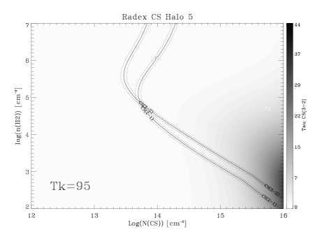
Figure 16: LVG diagrams of CS for Halo 5.

Additional support for the GMLs scenario comes from the kinetic temperature gradient and large NH₃ abundances of the high metastable inversion transitions. The sense of the temperature gradient can help to establish whether the shocks are due to the GMLs scenario or to the ejection of gas from the disk due to star formation. Temperature that decreases from the disk (low latitudes) to the halo in the GC region would indicate that the material is falling from the halo to the galactic disk supporting the GML scenario, because the post shocked gas which has cooled down is at larger latitude than the recently heated material at the shock front (see e.g., Fig. 16 of Genzel 1992). The gradient will be in the opposite way if the material is being ejected. We observed that the kinetic temperature is slightly larger in the foot point than in the top of the loop, which tentatively supports the loops scenario.

4.1.2 The two temperature components model in the CMZ clouds

In the CMZ (Disk X1-1, Disk X1-2, Disk X2-1, Disk X2-2, and Disk 2), our results are consistent with a two components model, with at least at two different temperatures, one cool and one warm (see Table 2 and 4). This result is in agreement with Hüttemeister et al. (1993a, 1998), who found that the data were consistent with two rotational temperature components: one cool ($\sim 25$ K) and other warm ($>100$ K). Furthermore, they found that for a typical GC molecular cloud, 25% of the gas has high temperatures, and this gas has low H₂ density; while the remaining 75% of the total gas mass is cooler at densities of $\geq 10^{4}$ cm^-3. Both gas components are in pressure equilibrium. Our result, on the other hand, indicates that there is as much gas in the low temperature component ($\sim$ 50%) as in the high temperature component ($\sim$ 50%). A possible explanation for such a discrepancy may be a selection effect: The positions from Hüttemeister et al. (1993a) are selected as intensity peaks in the CS maps from Bally et al. (1987), therefore these correspond to high density regions, as CS is a dense tracer. Our sources, on the contrary, correspond to shock positions, therefore expecting that the amount of warm molecular gas will be larger than at the positions from Hüttemeister et al. (1993a).

4.2 On the heating and cooling of the molecular gas in the GMLs and in the CMZ

Although the number of positions observed in the halo is rather limited, a remarkable result obtained in this work, is the single high kinetic temperature regime ($>95$ K) for the halo sources, in contrast with the two temperature regimens (cool and warm) present throughout the CMZ.

Therefore, the question that naturally arises is whether the cooling in the CMZ is more effective than in the halo positions, or if the heating mechanism in the GMLs is so efficient that the molecular gas has no time to be cooled down.

4.2.1 The cooling of the gas in the GC region

In the following, we describe the cooling rates for H₂ and CO emissions, and for the gas-dust coupling.

Goldsmith & Langer (1978) derived the temperature dependence of the total cooling rate for a variety of molecular hydrogen densities and at velocity gradient of 1 km s^-1 pc^-1 for the temperature range of 10 to 60 K. According to them, for $n(\mathrm{H_{2}})\leq 10^{3}\,\mathrm{cm}^{-3}$ the cooling is dominated by CO; and for $10^{3}\leq n(\mathrm{H_{2}})\leq 10^{5}\,\mathrm{cm}^{3}$, CI, O₂, and the isotopic species of CO, contribute with the 30% to 70% of the total cooling. We use the expressions of the total cooling rates ($\Lambda_{\mathrm{total}}$) derived by them for the different physical conditions of the molecular gas in the positions where this formulation is valid (see Table 9). Neufeld et al. (1995) and Neufeld & Kaufman (1993) derived the radiative cooling rates in a wider range of temperatures ($10\leq T\leq 2500$ K), and stated that the dominant coolants for the molecular interstellar gas are CO, H₂, O, and H₂O. The efficiency of the cooling depends of the gas temperature, the H₂ particle density, and the optical depth parameter $\tilde{N}(\mathrm{H_{2}})=n(\mathrm{H_{2}})/|dv/dz|$, where $dv/dz$ is the velocity gradient along the line of sight. The latter depends on the geometry and velocity structure assumed (see Table 1 in Neufeld & Kaufman 1993). Here we assume $\tilde{N}(\mathrm{\mathrm{H_{2}}})=N(\mathrm{H_{2}})/\Delta v$; where $N(\mathrm{H_{2}})$ is the $\mathrm{H_{2}}$ column density estimated in column 11 of Table 4, and $\Delta v$ is the measured line width of CS(2-1) (Table LABEL:SiO-CS-HNCO). We compute the total cooling rates according to their model in Table 9 by spline interpolation of the values for their molecular cooling function (Neufeld et al. 1995).

Later, Le Bourlot et al. (1999) derived the cooling rate by H₂ ($\Lambda_{\mathrm{H_{2}}}$) for a wider range of physical parameters ($100\leq T_{\mathrm{kin}}\leq 10^{4}$ K; $1\leq n(\mathrm{H_{2}})\leq 10^{8}$ cm^-3). We used the FORTRAN subroutine provided by them only towards the sources allowed by the parameters range, i.e., for the warm gas (Table 9).

The cooling rate for the coupling of the dust and gas is given by (Goldsmith & Langer 1978)

$$\Lambda_{\mathrm{gd}}=2.4\times 10^{-33}T_{g}^{1/2}(T_{g}-T_{d})n^{2}(\mathrm{H_{2}})\mathrm{\,erg\,s^{-1}cm^{-3}}\leavevmode\nobreak\ .$$ (1)

where the grains parameters (grain size and accommodation coefficient) where taken from Leung (1975). Hüttemeister et al. (1993a) argued that the cold gas component is coupled to the dust temperature at high densities, therefore, the dust in the GC region would be a cooling agent. They proposed that the density of the cold gas must be at least an order of magnitude higher than that of the hot gas; otherwise the hot gas would also cooled down. We find that the gas density of the hot component is only slightly lower than in the cold component (a factor $\sim 2-4$ from the CS data in Table 3). Although the gas-dust coupling becomes significant at $n(H_{2})\sim 10^{5}$ cm^-3 (Juvela & Ysard 2011), which is reached only in the cool component regime in few positions in the CMZ (Table 3), we estimated this cooling rate for all the positions (Table 9).

Estimating total cooling rates, e.g., following Goldsmith & Langer (1978), one should account for two factors: the depletion of coolant species, and the lack of processed gas in the halo. The depletion of the coolant species can increase the gas temperature at low and moderate densities of $n(\mathrm{H_{2}})\leq 10^{4}$ cm^-3. This effect was studied by Goldsmith (2001) in dark clouds. In the physical conditions of the GC, the depletion of the coolant species is unlikely due to the high densities and low temperatures which are needed to have this effect. Second, as we noted before, in the density range of the GC clouds, CI, O₂, and the isotopes of CO, contribute 30% to 70% of the total cooling. Riquelme et al. (2010a) found a high ¹²C/¹³C isotopic ratio towards the disk-halo connection regions (halo, disk X1) which they interpreted as non-processed gas being accreted towards the GC. If this interpretation is correct (since the gas in the loop is less processed than the gas in the CMZ), one would expect a lower metallicity and, hence, a less efficient cooling by molecular or atomic lines. On the other hand, a high isotopic ratio was also found towards the disk X1 positions, and those positions have indeed a cool temperature regime.

The low temperature regime toward the X1 orbit positions can be explained by the large H₂ cooling rate derived from Le Bourlot et al. (1999) and the large total cooling rates derived from Neufeld et al. (1995) (see Table 9). However, the cooling rate in the Halo positions are also large, and those positions do not present the cool temperature regime.

In the following, we estimate the heating rates affecting the GC region to study if a rise of the heating mechanism should be the responsible of the lack of low temperature regime in the halo sources.

4.2.2 The heating of the gas in the GC

We find high gas kinetic temperatures for basically all the observed positions of our sample. Therefore the heating mechanism responsible for the widespread high temperatures should apply for the gas in the entire GC region, with little effect on the dust. The heating mechanism in the GC should be different from that the heating of warm clouds (T${}_{\mathrm{kin}}>100$ K) in the disk, where the molecules are heated by collisions with hot dust, heated by embedded stars.

Several heating mechanisms have been proposed to explain the high kinetic temperatures in the GC region.

1. Cosmic rays heating: Heating by a large flux of low energy cosmic rays (Güsten et al. 1981; Morris et al. 1983; Hüttemeister et al. 1993a; Yusef-Zadeh et al. 2007a). This mechanism requires a cosmic ray ionization rate ($\zeta_{\rm CR}$) of one or two orders of magnitude larger than the Galactic value of 10${}^{-17}{\rm s}^{-1}$, which will influence also the gas-phase chemistry, increasing the atomic hydrogen due to the increased cosmic ray dissociation rate of H₂, and also molecular ion emission like HCO⁺. Yusef-Zadeh et al. (2007a, b) argue that such a high ionization rate is found in the GC region. From absorption lines of H${}_{3}^{+}$ originating from a diffuse, hot molecular component in the CMZ, Goto et al. (2008) estimated an ionization rate of $\sim 10^{-15}\,s^{-1}$. We assume a similar value in the gas observed by us, although it is presumably denser and cooler. The heating rate depends on $n$ and $\zeta_{\rm CR}$. It is difficult to derive it for each observed position, and this mechanism cannot be ruled out.

2. X-ray heating: Heating by an extended diffuse source of soft X-ray emission (Watson et al. 1981) is unlikely since the X-ray emission is less extended than the NH₃ emission, and there is no obvious source for the required luminosity in the extended soft X-ray emission (Morris et al. 1983). Heating by an extremely hot plasma emitting X-rays. Nagayama et al. (2007) found that the NH₃ emitting region in the CMZ, with $T_{\rm kin}=20-80$ K and $T_{\rm kin}>80$ K, is surrounded, in the longitude-velocity space, by a high-pressure region (Sawada et al. 2001), where the gas is less dense and hotter ($n(H_{2})<10^{3}\,\mathrm{cm^{-3}}$, $T_{\rm kin}>100$ K). Because the high pressure region is found to be coincident with the hot emitting X-rays, they argued that the thermal energy radiated from the hot plasma emitting X-ray plasma can heat the gas in the high pressure region. The heating rate due to this mechanism is very uncertain, but Ao et al., (2012, in prep.) argue that this mechanisms is not able to account for the high kinetic temperatures in the GC region.

3. Ion-Slip heating: The GC is pervaded by a magnetic field of few mG (see e.g., Ferrière et al. 2007), and their presence can also influence the heating of the GC. The ion-slip heating has been proposed for the molecular clouds in the GC region, where the heating rate depends on the magnetic field $B$, ionization rate, neutral number density $n_{n}$, ion number density $n_{i}$, number of collision per second, the reduced mass of the ions and neutrals, and the scale of the cloud $R$ (in pc) (see, Scalo 1977). Because of the uncertainty of some on these values for each observed position, it is difficult to estimate the heating rate.

4. Ultraviolet heating: The high NH₃ abundances in the GC region require effective shielding from UV radiation because ammonia is easily photodisociated by ultraviolet radiation (Rodríguez-Fernández et al. 2001). This is also confirmated by the large abundance of the HNCO molecule, which is also photodissociated by UV radiation. We discard UV heating in the GC region.
   HNCO could be formed via gas phase reactions, but formation in grains seems to be more efficient (see e.g., Martín et al. 2008, and references therein). Presumably this molecule is released to the ISM by grain erosion and/or disruption by shocks (Zinchenko et al. 2000), and is easily photodissociated by UV radiation. The shocks that release the molecule from the grain mantles should be slow enough to not dissociated the molecule. We find that the X(HNCO) is low in the Disk X1-1 source, where we expect shocks, but no UV emission. Also we can see an enhancement toward the Halo 1 source (cloud number 2), and the Disk X2-1 source, which could be due to the shocks present in these regions, are strong enough to evaporate the molecule from the grain mantles but too slow to not dissociate the HNCO. This molecule can be used to trace the shocks properties throughout the GC region.

5. Shocks: The dissipation of mechanical turbulence through shocks would offer a compelling answer, because the GC region shows an ubiquitous presence of shocks, as traced by the SiO emission (Martín-Pintado et al. 2000; Riquelme et al. 2010b). The heating rate due to the dissipation of turbulence (of velocity $v_{t}$ on a spatial scale of $R_{c}$) is given by (Black 1987)

   $$\Gamma_{\mathrm{turb}}\approx 3.5\times 10^{-28}v_{t}^{3}n_{H}\left(\frac{1\mathrm{pc}}{R_{c}}\right)\mathrm{\,erg\,s^{-1}cm^{-3}}$$ (2)

   We derive the heating rate of the dissipation of turbulence for each position in Table 9. We use $R_{c}=5$ pc (Rodríguez-Fernández et al. 2001). It is important to note that this equation is highly dependent of $v_{t}$, therefore if the molecular clouds are not resolved in the beam size, the heating rate would be overestimated.
   The origin of this turbulence in the positions studied in this work, can be the following: the large scale dynamics in a barred potential model (Binney et al. 1991) can produce the shocks found towards the high velocity clouds associated with the X1 orbits (in the 1.3 complex, and Sgr C). This is supported by the higher kinetic temperatures found in the disk X1 sources than in the disk X2 sources (Table 4). In our “halo” positions the shocks can be produced by the GMLs scenario, which is supported by the broad velocity width at the foot point of the loops. However, high kinetic temperatures and the large SiO emission are widespread throughout all the GC region. Supernova or hypernova explosions could cause for the high temperature found in the lower velocity components (in our notation, disk X2) of the 1^∘.3 complex (Tanaka et al. 2007). For the lower longitudes in the CMZ, the heating could be explained by interactions with SNRs close to Sgr A and also with non-thermal filaments in the radio arc, and cloud-cloud collisions, and expanding bubbles in the vicinity of Sgr B Martín-Pintado et al. (1997). Cloud-cloud collisions were also proposed in the GC region (Wilson et al. 1982), which is favored by the large linewidth typical in the GC clouds. Güsten et al. (1985) argue that if this mechanism is acting in the molecular gas, the linewidth and the temperatures should be correlated. Mauersberger et al. (1986a) found such a correlation for the clouds observed in the GC, which would support this mechanism. Like Hüttemeister et al. (1993a), we do not confirm such a clear correlation between the rotational temperature associated with the inversion transitions (2,2), (4,4), and (5,5) (Table 2) and the Doppler width of our sources (see Fig 3). For the few observed positions we can neither confirm nor reject the cloud-cloud collisions as primary heating mechanism in our sources.

The heating rates derived from Eq. 2 for the halo and disk positions are similar. Therefore, it is probably that this mechanism by itself is not causing the lack of the low temperature regimen observed in the halo positions. An extra heating input would be required for the halo positions. Torii et al. (2010a) propose that the gas in the foot point of the GML is heating by C-shocks, and that the warmest region of the foot point (the “U shape”) would also be heated by magnetic reconnection or by upward flowing gas bounced by the narrow neck in the foot point. They estimated that the total available energy (considering the magnetic and gravitational energy) injected to the U shape is $1.8-2.6\times 10^{37}\mathrm{ergs^{-1}}$ in $\sim 10^{6}$ years. Consider a cloud size of 3 pc radius, as estimated by Torii et al. (2010a), the heating rate is $\Gamma\sim 3.9-7.8\times 10^{-21}$ erg cm^-3 s^-1. This heating rate is negligible in comparison with the values obtained from the dissipation of turbulence alone. Alternatively, the CMZ can be understood as a highly turbulent medium, where many phenomena are taking place (shocks produced by Galactic potential, SN explosions, star formation, interaction with non-thermal filaments, cosmic rays, the presence of a supermassive black hole, etc) and coexist in the central few hundred parsec of the Galaxy. All of these phenomena modify the physical parameter of the region. The two kinetic temperature regimes present in this region, which are in pressure equilibrium (Hüttemeister et al. 1998), could be the results of the interplay of the different phenomena mentioned above. On contrary, in the GMLs scenario, the gas goes down towards the Galactic plane following the magnetic field lines, which lead a tidy movement of the gas producing shocks front at the foot point of the loops. The continuous shock at the foot point is not affected by other phenomena (like, e.g., star formation), therefore the gas is continuously heated. High resolution maps of the foot point of the GMLs are needed not only to confirm this hypothesis but also to resolve the linewidth of the molecular clouds to better estimate the heating rate for dissipation of turbulence (Eq. 2). Summarizing, in spite of the limited number of positions studied in this work, we propose that the high kinetic temperature found in all of the sources are produced by shocks. We discarded UV heating due to the large abundance of HNCO and NH₃ molecule. From our data it is not possible to confirm or rule out x-ray and ion-slip heating.

Figure 3: $T_{rot}$ is plotted versus the average velocity linewidth from all the metastable inversion transitions. The $T_{rot}$ correspond to the values in bold from the Table 2

5 The ammonia ortho-to-para ratio and its implications on kinetic temperatures now and there

Radiative and collisional transitions between ortho-NH₃ $(K=0,3,6,9...)$ and para-NH₃ $(K=1,2,4,5...)$ are forbidden because of their different nuclear spins. The time scale of conversion between ortho and para species is $10^{6}$ yrs in the gas phase (Cheung et al. 1969). Therefore ortho-NH₃ and para-NH₃ can be almost treated as different species. The spin temperatures between ortho and para-NH₃, or the ortho/para ratio, may reflect the conditions at the time of the formation of NH₃, while rotational temperature within the same species reflect present conditions (Ho & Townes 1983; Umemoto et al. 1999).

A ratio of 1.0 would be expected if NH₃ is formed in the gas phase reactions at high temperatures, and a larger value could be explained by a formation on cold dust grains and a subsequent release into the gas phase. For temperatures of about 10 K, the typical temperature of cold dust, the ortho-to-para ratio will be larger than 2.

Dulieu (2011), however, points out that there might be a differential desorption on ortho and para molecules from dust grains and that this, and not the formation process, determines the gas phase ortho/para ratios.

From the LVG analysis of the ammonia molecule, we derive an ortho-to-para ratio average for all of our sources of $0.70$ with a standard deviation of $0.20$ (see Table 7). In this calculation, we take into account only the warm component of the para-NH₃ with the ortho-NH₃. While the ortho-NH₃ transitions are probably tracing higher kinetic temperatures than the para-species (see Table 10), the ortho-to-para ratio derived using RADEX for the warm kinetic temperature component approaches to the statistical equilibrium value. This result is consistent with Hüttemeister et al. (1993a) estimation of the $(3,3)$ column density. Non thermal emission has been predicted for the NH₃ (3,3) line by Walmsley & Ungerechts (1983), and has been observed e.g. by Mauersberger et al. (1986a, b). Also the $(6,6)$ line might be a maser source in some case (Lebrón et al. 2011). Our RADEX calculations were made assuming a background of 2.7 K. We have verified that in our models the ortho lines tend to be weak masers for a large part of our parameter space.

Table 7: Ortho-to-para NH₃ ratio from LVG model

Source	a	$N(o-NH_{3})/N(p-NH_{3})^{b}$
Halo1	1	$0.83$
	2	$0.63$
	3	$0.68$
Halo4	1	$0.48$
DiskX1-1	1	$1.0$
DiskX2-1	1	$0.76$
DiskX1-2	1	$0.93$
DiskX2-2	1	$0.76$
Disk1	1	$2.02^{c}$
	2	$0.72^{c}$
Disk2	1	$0.59$
	2	$0.63$
	3	$0.34$

• ^a Cloud number defined by the different velocity components.

• ^a We take into account only the warm component of the para-NH₃ with the ortho-NH₃ (see text for details).

• ^c This value was not considered in the average of the ortho-to-para ratio, because it is possible that this position does not have the high kinetic temperature regimen.

6 Conclusions

1. We have used the metastable inversion transitions of NH₃ from $(J,K)=(1,1)$ to $(6,6)$ to derive the gas kinetic temperature toward six positions selected in the Galactic central disk and for higher latitude molecular gas. We also observed other molecules like SiO, HNCO, CS, C³⁴S, C¹⁸O, and ¹³CO, to derive the densities and to trace different physical processes (shocks, photodissociation, dense gas) which was used to reveal the heating mechanisms affecting the molecular gas in these regions.

2. The GC molecular gas consists of roughly two kinetic temperature components in the CMZ. Only the warm kinetic temperature regime is found in the “halo” positions, and in the Disk 2 position, which corresponds to Sgr B2. The results obtained in this paper apply for the disk and halo positions defined in this work within the GC region, and do not represent the conditions for the Galaxy as a whole.

3. The kinetic temperatures are high, not only in the typical GC clouds, but also in the high latitude and high velocity clouds observed in this paper.

4. Shocks are a compelling heating mechanism of the molecular clouds in the GC region. This is supported by the high gas kinetic temperature and by the increased SiO abundance in the location where shock are expected. Due to the fragile nature of the HNCO (enhanced by shock but easily photodissociated by UV radiation and strong shocks), this molecule could be used to reveal the characteristic of the shock. Other heating mechanisms previously proposed for the GC, however, cannot been ruled out.

5. The high kinetic temperatures found in both, the X1 orbits and in the foot point of the GMLs, seem to support to the large scale dynamics induced by the bar potential, and the GMLs scenario as origins for the shocks respectively.

Appendix A Complementary Tables

Table 8: Fractional abundances of NH₃ with respect to SiO, HNCO, CS, C³⁴S, and of SiO and HNCO with respect to CS and C³⁴S

Source	$n^{a}$	$\frac{N(NH_{3})}{N(SiO)}$	$\frac{N(NH_{3})}{N(HNCO)}$	$\frac{N(NH_{3})}{N(CS)}$	$\frac{N(NH_{3})}{N(C^{34}S)}$	$\frac{N(SiO)}{N(CS)}$	$\frac{N(SiO)}{N(C^{34}S)}$	$\frac{N(HNCO)}{N(CS)}$	$\frac{N(HNCO)}{N(C^{34}S)}$	$\frac{N(SiO)}{N(HNCO)}$
Halo1	1	$11.97\pm 3.64$	$53.64\pm 16.28$	$3.99\pm 1.21$		$>0.33$		$>0.07$		$>4.48$
	2	$9.11\pm 2.68$	$14.59\pm 3.09$	$2.32\pm 0.41$	$33.40\pm 7.84$	$0.25\pm 0.09$	$3.67\pm 1.35$	$0.16\pm 0.04$	$2.29\pm 0.70$	$1.60\pm 0.57$
	3	$3.41\pm 2.67$		$1.01\pm 0.76$		$0.29\pm 0.31$
Halo2	1					$0.14\pm 0.15$	$1.69\pm 2.01$	$0.29\pm 0.31$	$3.47\pm 4.05$	$0.49\pm 0.53$
	2					$>0.12$
Halo3	1					$0.17\pm 0.09$	$2.60\pm 1.50$	$0.20\pm 0.10$	$3.08\pm 1.58$	$0.85\pm 0.42$
	2							$0.33\pm 0.17$	$3.89\pm 2.58$
Halo4	1	$32.32\pm 18.12$	$8.60\pm 3.46$	$5.46\pm 2.84$	$81.43\pm 49.50$	$0.17\pm 0.12$	$2.52\pm 1.97$	$0.64\pm 0.38$	$9.47\pm 6.41$	$0.27\pm 0.17$
Halo5	1					$0.19\pm 0.07$	$2.18\pm 0.80$	$0.49\pm 0.15$	$5.60\pm 1.64$	$0.39\pm 0.14$
DiskX1-1	1	$8.91\pm 2.30$	$12.46\pm 2.51$	$2.69\pm 0.65$	$52.80\pm 13.87$	$0.30\pm 0.08$	$5.93\pm 1.74$	$0.22\pm 0.05$	$4.24\pm 1.04$	$1.40\pm 0.34$
DiskX2-1	1	$14.33\pm 6.28$	$5.57\pm 1.70$	$2.48\pm 1.04$	$58.46\pm 24.92$	$0.17\pm 0.10$	$4.08\pm 2.44$	$0.44\pm 0.22$	$10.49\pm 5.33$	$0.39\pm 0.20$
DiskX1-2	1	$14.32\pm 2.76$	$9.83\pm 1.76$	$2.78\pm 0.48$	$42.41\pm 6.94$	$0.19\pm 0.04$	$2.96\pm 0.62$	$0.28\pm 0.06$	$4.31\pm 0.86$	$0.69\pm 0.15$
DiskX2-2	1	$111.3\pm 34.7$	$14.52\pm 3.28$	$2.60\pm 0.70$	$29.67\pm 7.91$	$0.02\pm 0.01$	$0.27\pm 0.08$	$0.18\pm 0.04$	$2.04\pm 0.47$	$0.13\pm 0.04$
Disk1	1	$6.67\pm 0.00$	$>2.84$	$>1.11$	$93.33\pm 0.00$	$>0.17$	$>14.00$	$>0.39$	$>32.83$	$>0.43$
	2	$17.28\pm 6.91$	$4.59\pm 1.32$	$1.95\pm 0.72$	$45.96\pm 18.58$	$0.11\pm 0.06$	$2.66\pm 1.51$	$0.42\pm 0.20$	$10.02\pm 4.98$	$0.27\pm 0.13$
Disk2	1	$74.31\pm 23.50$		$24.65\pm 7.26$	$71.03\pm 20.94$	$0.33\pm 0.14$	$0.96\pm 0.41$
	2	$89.23\pm 0.19$	$>1.90$	$30.43\pm 0.06$	$88.60\pm 0.19$	$>0.34$	$>0.99$	$>16.01$	$>46.63$	$>0.02$
	3			$14.30\pm 1.86$

• ^a Cloud number defined by the different velocity components.

Table 9: Estimation of heating and cooling rates for each source

Source	$n^{a}$	$T_{kin}$	$n(H_{2})$	$\Lambda_{total}^{b,e}$	$\Lambda_{total}^{c,e}$	$\Lambda_{H_{2}}^{d,e}$	$\Lambda_{gd}^{d}$	$\Gamma_{turb}^{e}$
		[K]	[$\times 10^{4}$cm-3]
Halo1	1	115	$1.00$		14.0	0.78	0.018	27.5
Halo1	2	90	$8.49$		242	4.36	0.86	58.4
Halo1	3	135	$1.58$		46.8	31.4	0.057	12.9
Halo2	1	113	$1.26$		21.6	0.015	0.028	31
Halo2	2	113	$0.97$		13.3	0.82	0.016	16.5
Halo3	1	113	$1.50$		30.7	1.3	0.039	62.6
Halo3	2	113	$3.55$		136	3.1	0.22	178
Halo4	1	95	$2.75$		44.9	1.4	0.10	41
Halo5	1	95	$7.47$		210	3.9	0.74	51.4
Disk-X1	1	38	$13.0$	1.5	36.7		0.081	849
		300	$3.55$		534	261	0.79	232
Disk-X2	1	38	$5.62$	1.5	12.7		0.015	234
		100	$2.70$		48.5	1.2	0.11	113
Disk-X1	2	52	$13.3$	3.6	101		0.51	76.3
		215	$5.62$		746	112	1.3	32.2
Disk-X2	2	28	$14.1$	0.60	16.5		0.57	158
		95	$6.20$		150	3.3	0.51	69.4
Disk1	1	23	$1.12$	0.071	1.26		0.005	5.29
		154	$0.16$		1.37	0.51	0.001	0.76
Disk1	2	38	$4.57$	0.28	25.8		0.010	31.4
		82	$2.51$		45.1		0.064	17.3
Disk2	1	68	$4.97$	1.3	48.6		0.17	250
		200	$2.47$		179	34	0.23	124
Disk2	2	145	$2.51$		55.8	8.1	0.16	32.5
Disk2	3	50	$15.8$	3.2	86.8		0.60	129
		80	$11.6$		224		1.3	94.7

• ^a Cloud number defined by the different velocity components.

• ^b from Goldsmith & Langer (1978).

• ^c from Neufeld et al. (1995); Neufeld & Kaufman (1993)

• ^d using program provided by Le Bourlot et al. (1999).

• ^e [$\times 10^{-21}\mathrm{erg\,s^{-1}cm^{-3}}$]

Table 10: Column density derived for NH3 (3,3) and NH3 (6,6) using RADEX

Source	a	n(H2)	T(kin)	N(ortho-NH3)
Halo1	1	$1.00\times 10^{4}$	$>300$	$1\times 10^{14}$
Halo1	2	$8.49\times 10^{4}$	$>300$	$1.26\times 10^{14}$
Halo1	3	$1.58\times 10^{4}$	$>300$	$0.45\times 10^{14}$
Halo4	1	$2.75\times 10^{4}$	$>170$	$0.95\times 10^{14}$
DiskX1-1	1	$3.55\times 10^{4}$	$>300$	$1.58\times 10^{14}$
DiskX2-1	1	$2.70\times 10^{4}$	$>200$	$2.51\times 10^{14}$
DiskX1-2	1	$5.62\times 10^{4}$	$>280$	$1.41\times 10^{14}$
DiskX2-2	1	$6.20\times 10^{4}$	$265$	$0.76\times 10^{14}$
Disk1	1	$0.16\times 10^{4}$	$>300$	$0.32\times 10^{14}$
Disk1	2	$2.51\times 10^{4}$	$>300$	$0.32\times 10^{14}$
Disk2	1	$2.47\times 10^{4}$	$200$	$8.32\times 10^{14}$
Disk2	2	$2.51\times 10^{4}$	$>300$	$12.6\times 10^{14}$
Disk2	3	$11.6\times 10^{4}$	$130$	$4.79\times 10^{14}$

• ^a Cloud number defined by the different velocity components.

Table 11: Results from Gaussian fit and optical depth from NH₃ method.

Source	Cloud	Transition	$v_{\rm LSR}$	TMB	$\Delta v_{1/2}$	Integrated intensitye	rms	$\tau$
	numberf	(j,k)	[ km s-1]	[K]	[ km s-1]	[K  km s-1]	[mk]
Halo 1	1	(1,1)	$85.6\pm 0.4$	$0.10$	$29.0\pm 0.4$	$3.19\pm 0.04$	$52$	$<0.40$
	2	(1,1)	$115.8\pm 0.4$	$0.32$	$23.6\pm 0.4$	$7.91\pm 0.04$	$52$	$0.10\pm 0.09$
	3	(1,1)	$139.3\pm 0.4$	$0.09$	$18.8\pm 0.4$	$1.77\pm 0.04$	$52$	$<0.64$
	1	(2,2)	$83.1\pm 0.4$	$0.07$	$37.8\pm 0.4$	$2.94\pm 0.04$	$51$	$<0.86$
	2	(2,2)	$116.7\pm 0.4$	$0.35$	$18.4\pm 0.4$	$6.77\pm 0.04$	$51$	$0.21\pm 0.01$
	3	(2,2)	$147.1\pm 0.4$	$0.06$	$35.5\pm 0.4$	$2.29\pm 0.04$	$51$	$4.9\pm 2.0^{d}$
	1	(3,3)	$87.7\pm 0.4$	$0.22$	$38.8\pm 0.4$	$9.23\pm 0.07$	$51$	$0.10\pm 0.03$
	2	(3,3)	$117.2\pm 0.4$	$0.85$	$16.8\pm 0.4$	$15.16\pm 0.07$	$51$	$0.10\pm 0.03$
	3	(3,3)	$138.6\pm 0.4$	$0.19$	$20.8\pm 0.4$	$4.29\pm 0.07$	$51$	$0.16\pm 0.01$
	1	(4,4)	$82.0\pm 0.4$	$0.06$	$32.9\pm 0.4$	$2.03\pm 0.02$	$50$
	2	(4,4)	$118.7\pm 0.4$	$0.23$	$21.5\pm 0.4$	$5.34\pm 0.02$	$50$
	3	(4,4)	$137.4\pm 0.4$	$0.05$	$16.6\pm 0.4$	$0.91\pm 0.02$	$50$
	1	(5,5)	$87.7^{a}$	$0.12^{b}$	$38.8^{a}$	$0.467^{b}$	$41$
	2	(5,5)	$115.7\pm 0.4$	$0.15$	$12.4\pm 0.9$	$1.92\pm 0.13$	$41$
	3	(5,5)	$131.0\pm 0.9$	$0.06$	$11.9\pm 3.2$	$0.74\pm 0.09$	$41$
	1	(6,6)	$87.7^{a}$	$0.13^{b}$	$38.8^{a}$	$0.613^{b}$	$41$
	2	(6,6)	$120.5\pm 0.8$	$0.30$	$17.3\pm 2.1$	$5.48\pm 0.61$	$41$
	3	(6,6)	$138.5\pm 1.9$	$0.12$	$14.4\pm 2.9$	$1.78\pm 0.54$	$41$
Halo 4	1	(1,1)	$196.4\pm 0.9$	$0.22$	$30.2\pm 2.1$	$6.99\pm 0.42$	$83$	$<0.31$
	1	(2,2)	$194.7\pm 1.1$	$0.19$	$34.1\pm 2.9$	$6.74\pm 0.47$	$84$	$1.72\pm 0.53$
	1	(3,3)	$195.5\pm 0.5$	$0.37$	$20.3\pm 1.2$	$7.93\pm 0.38$	$80$	$<0.31$
	1	(4,4)	$194.5\pm 1.1$	$0.09$	$16.0\pm 2.9$	$1.44\pm 0.20$	$49$
	1	(5,5)	$195.5^{a}$	$0.15^{b}$	$20.3^{a}$	$0.417$	$50$
	1	(6,6)	$199.4\pm 1.7$	$0.09$	$24.3\pm 4.0$	$2.26\pm 0.32$	$51$
Disk X1-1	1	(1,1)	$183.1\pm 1.0$	$0.20$	$48.1\pm 2.2$	$10.43\pm 0.45$	$74$	$0.86\pm 0.27$
	1	(2,2)	$182.9\pm 1.3$	$0.15$	$32.1\pm 2.6$	$5.10\pm 0.38$	$71$	$0.10\pm 0.11$
	1	(3,3)	$184.1\pm 0.4$	$0.43$	$34.8\pm 1.0$	$15.88\pm 0.39$	$71$	$0.10\pm 0.02$
	1	(4,4)	$188.1\pm 1.1$	$0.14$	$24.7\pm 2.2$	$3.66\pm 0.33$	$74$
	1	(5,5)	$187.1\pm 1.7$	$0.09$	$36.4\pm 4.1$	$3.56\pm 0.34$	$63$
	1	(6,6)	$188.3\pm 1.1$	$0.17$	$35.0\pm 2.6$	$6.25\pm 0.41$	$59$
Disk X2-1	1	(1,1)	$96.4\pm 0.4$	$0.48$	$40.8\pm 1.0$	$20.91\pm 0.42$	$74$	$<0.84$
	1	(2,2)	$96.5\pm 0.5$	$0.32$	$30.7\pm 1.4$	$10.36\pm 0.38$	$71$	$0.10\pm 0.02$
	1	(3,3)	$98.1\pm 0.2$	$0.74$	$32.9\pm 0.6$	$25.95\pm 0.39$	$71$	$0.10\pm 0.01$
	1	(4,4)	$96.0\pm 0.6$	$0.19$	$15.7\pm 1.7$	$3.16\pm 0.28$	$74$
	1	(5,5)	$98.6\pm 2.2$	$0.09$	$41.5\pm 4.6$	$3.91\pm 0.37$	$63$
	1	(6,6)	$103.4\pm 1.1$	$0.17$	$30.8\pm 2.6$	$5.70\pm 0.40$	$59$
Disk X1-2	1	(1,1)	$69.1\pm 0.5$	$0.32$	$22.7\pm 1.3$	$7.77\pm 0.37$	$78$	$0.10\pm 0.03$
	1	(2,2)	$69.4\pm 0.4$	$0.32$	$14.5\pm 1.3$	$4.99\pm 0.33$	$80$	$0.10\pm 0.06$
	1	(3,3)	$69.1\pm 0.2$	$0.87$	$17.3\pm 0.6$	$16.10\pm 0.42$	$91$	$0.10\pm 0.04$
	1	(4,4)	$69.9\pm 0.4$	$0.25$	$12.2\pm 1.4$	$3.23\pm 0.26$	$71$
	1	(5,5)	$67.0\pm 0.7$	$0.13$	$13.1\pm 1.4$	$1.84\pm 0.20$	$62$
	1	(6,6)	$74.1\pm 0.6$	$0.24$	$17.8\pm 1.7$	$4.58\pm 0.33$	$61$
Disk X2-2	1	(1,1)	$-50.2\pm 0.8$	$0.25$	$37.9\pm 1.9$	$10.22\pm 0.46$	$78$	$1.00\pm 0.29$
	1	(2,2)	$-53.0\pm 1.2$	$0.15$	$22.1\pm 3.1$	$3.51\pm 0.39$	$80$	$<0.28$
	1	(3,3)	$-47.1\pm 0.6$	$0.35$	$22.9\pm 1.4$	$8.41\pm 0.45$	$91$	$<0.23$
	1	(4,4)	$-54.1\pm 0.6$	$0.14$	$6.7\pm 1.5$	$0.99\pm 0.18$	$71$
	1	(5,5)	$-47.1^{a}$	$0.19^{b}$	$22.9^{a}$	$0.55^{b}$	$62$
	1	(6,6)	$-49.3\pm 2.8$	$0.07$	$21.0\pm 4.9$	$1.31\pm 0.31$	$61$
Disk 1	1	(1,1)	$64.5\pm 0.4$	$0.08$	$20.0\pm 0.4$	$1.73\pm 0.03$	$61$	$<1.25$
	2	(1,1)	$78.2\pm 0.4$	$0.16$	$18.4\pm 0.4$	$3.05\pm 0.03$	$61$	$<0.34$
	1	(2,2)	$59.3\pm 0.8$	$0.08$	$5.1\pm 1.6$	$0.45\pm 0.15$	$63$	$<1.35$
	2	(2,2)	$73.4\pm 0.5$	$0.16$	$8.5\pm 1.5$	$1.47\pm 0.20$	$63$	$<0.26$
	1	(3,3)	$56.5\pm 1.0$	$0.11$	$11.7\pm 3.1$	$1.36\pm 0.27$	$66$	$<0.56$
	2	(3,3)	$72.4\pm 0.6$	$0.21$	$14.9\pm 0.5$	$3.41\pm 0.03$	$66$	$<0.32$
	1	(4,4)	$56^{a}$	$0.16^{b}$	$11.7^{a}$	$0.33^{b}$	$53$
	2	(4,4)	$72^{a}$	$0.16^{b}$	$15.0^{a}$	$0.38^{b}$	$53$
	1	(5,5)	$56^{a}$	$0.14^{b}$	$11.7^{a}$	$0.29^{b}$	$47$
	2	(5,5)	$72^{a}$	$0.14^{b}$	$15.0^{a}$	$0.33^{b}$	$47$
	1	(6,6)	$56^{a}$	$0.15^{b}$	$11.7^{a}$	$0.39^{b}$	$50$
	2	(6,6)	$72^{a}$	$0.15^{b}$	$15.0^{a}$	$0.44^{b}$	$50$
Disk 2	1	(1,1)	$46.1\pm 0.1$	$2.2$	$24.1\pm 0.3$	$56.34\pm 0.65$	$94$	$0.10\pm 0.10^{c}$
	2	(1,1)	$73.9\pm 0.1$	$3.0$	$18.4\pm 0.2$	$58.21\pm 0.40$	$94$	$3.00\pm 0.10^{c}$
	3	(1,1)	$90.2\pm 0.1$	$3.6$	$16.7\pm 0.1$	$64.73\pm 0.33$	$94$	$0.10\pm 0.10^{c}$
	1	(2,2)	$44.9\pm 0.1$	$1.8$	$22.6\pm 0.4$	$42.52\pm 0.58$	$106$	$0.10\pm 0.01$
	2	(2,2)	$74.3\pm 0.2$	$3.2$	$17.2\pm 0.3$	$57.55\pm 1.43$	$106$	$0.15\pm 0.01$
	3	(2,2)	$94.1\pm 0.3$	$2.1$	$18.6\pm 0.5$	$41.28\pm 1.31$	$106$	$0.10\pm 0.01$
	1	(3,3)	$48.8\pm 0.1$	$3.4$	$28.7\pm 0.3$	$103.6\pm 0.8$	$98$	$0.10\pm 0.10^{c}$
	2	(3,3)	$74.5\pm 0.1$	$14$	$14.4\pm 0.1$	$216.2\pm 0.7$	$98$	$0.10\pm 0.10^{c}$
	3	(3,3)	$95.8\pm 0.1$	$2.7$	$18.6\pm 0.2$	$52.42\pm 0.51$	$98$	$0.10\pm 0.10^{c}$
	1	(4,4)	$50.1\pm 0.6$	$0.8$	$32.5\pm 1.3$	$26.23\pm 0.97$	$74$
	2	(4,4)	$74.0\pm 0.1$	$3.1$	$15.0\pm 0.2$	$49.35\pm 1.03$	$74$
	3	(4,4)	$96.2\pm 0.6$	$0.48$	$20.0\pm 1.2$	$10.24\pm 0.57$	$74$
	1	(5,5)	$53.5\pm 0.1$	$0.40$	$35.2\pm 0.5$	$14.90\pm 0.20$	$57$
	2	(5,5)	$73.0\pm 0.1$	$2.0$	$15.9\pm 0.1$	$33.44\pm 0.28$	$57$
	3	(5,5)	$97.3\pm 0.6$	$0.18$	$16.3\pm 1.4$	$3.10\pm 0.24$	$57$
	1	(6,6)	$56.5\pm 0.3$	$0.69$	$15.9\pm 0.8$	$11.80\pm 0.53$	$51$
	2	(6,6)	$75.7\pm 0.1$	$2.4$	$15.2\pm 0.2$	$38.76\pm 0.48$	$51$
	3	(6,6)	$96^{a}$	$0.15^{b}$	$18.6^{a}$	$0.51^{b}$	$51$

Table 11: continued.

• ^a no detected. Value taken as reference from the (3,3) transition.

• ^b upper limits.

• ^c method NH₃ did not converge properly.

• ^d the fit is not good, due to the no convergence of the method.

• ${}^{e}\int T_{{\rm MB}}dv$.

• ^f In each source, different velocity components define different clouds.

Table 12: Gaussian fits and column densities for SiO, C³⁴S, HNCO

Source	Species	Velocity Center	$\Delta_{v}$	$T_{\rm A}$	$\int T_{\rm A}dv^{c}$	rms	N
		LSR [ km s-1]	[ km s-1]	[K]	[K  km s-1]	[mK]	[cm-2]
Halo 1	SiO (2-1)	$88.0\pm 0.1$	$33.5\pm 1.0$	$0.096$	$3.41\pm 0.01$	$4.5$	$5.73\pm 0.01\times 10^{12}$
		$117.8\pm 0.1$	$17.9\pm 0.1$	$0.993$	$18.96\pm 0.08$	$4.5$	$31.82\pm 0.14\times 10^{12}$
		$133.5\pm 0.3$	$20.7\pm 0.7$	$0.174$	$3.83\pm 0.02$	$4.5$	$6.43\pm 0.03\times 10^{12}$
	29SiO(2-1)	$119.7\pm 0.6^{a}$	$17.2\pm 1.3$	$0.085$	$1.55\pm 0.11$	$6.3$	$2.66\pm 0.19\times 10^{12}$
	30SiO (2-1)	$120.0\pm 0.8^{a}$	$17.4\pm 1.9$	$0.063$	$1.16\pm 0.11$	$5.9$	$2.04\pm 0.19\times 10^{12}$
	CS (2-1)	$84.8\pm 0.5$	$27.5\pm 1.2$	$0.211$	$6.2\pm 1.8$	$0.2$
		$116.5\pm 0.1$	$17.1\pm 0.1$	$1.627$	$29.7\pm 0.2$	$0.2$
		$130.4\pm 0.2$	$18.2\pm 0.6$	$0.364$	$7.06\pm 0.09$	$0.2$
	CS (3-2)	$83.1\pm 4.1$	$23.3\pm 4.1$	$0.075$	$1.86\pm 0.96$	$9.6$
		$116.5\pm 4.1$	$15.4\pm 4.1$	$1.517$	$24.80\pm 0.96$	$9.6$
		$130.7\pm 4.1$	$11.2\pm 4.1$	$0.279$	$3.34\pm 0.96$	$9.6$
	C34S (2-1)	$-$	$-$	$-$	$-$	$-$	$-$
		$117.\pm 0.3$	$18.8\pm 0.8$	$0.138$	$2.75\pm 0.10$	$5.6$	$9.51\pm 0.34\times 10^{12}$
		$-$	$-$	$-$	$-$	$-$
	HNCO	$83.2\pm 2.0$	$15.2\pm 4.0$	$0.023$	$0.37\pm 0.09$	$5.2$	$10.8\pm 2.6\times 10^{12}$
		$117.2\pm 0.4$	$21.7\pm 1.1$	$0.119$	$2.75\pm 0.11$	$5.2$	$81.0\pm 3.4\times 10^{12}$
		-	-	-	-	-
	C18O(1-0)	$89.0\pm 0.9$	$26.8\pm 1.9$	$0.057$	$1.62\pm 0.10$	$4.7$	$1.11\pm 0.07\times 10^{15}$
		$115.9\pm 0.2$	$18.8\pm 0.6$	$0.108$	$2.17\pm 0.04$	$4.7$	$1.49\pm 0.03\times 10^{15}$
		$140.7\pm 1.4$	$16.6\pm 3.8$	$0.022$	$0.38\pm 0.07$	$4.7$	$0.26\pm 0.05\times 10^{15}$
	13CO(1-0)	$85.0\pm 0.4$	$37.6\pm 1.4$	$0.344$	$13.77\pm 0.4$	$12.0$	$0.94\pm 0.03\times 10^{15}$
		$114.2\pm 0.2$	$13.3\pm 0.4$	$0.628$	$8.92\pm 0.5$	$12.0$	$0.61\pm 0.03\times 10^{15}$
		$133.7\pm 1.4$	$27.2\pm 3.1$	$0.167$	$4.84\pm 0.6$	$12.0$	$0.33\pm 0.04\times 10^{15}$
		$169.5\pm 2.3$	$23.6\pm 6.0$	$0.049$	$1.23\pm 0.26$	$12.0$	$0.08\pm 0.02\times 10^{15}$
Halo 2	SiO (2-1)	$-84.7\pm 1.1$	$25.5\pm 0.8$	$0.046$	$1.25\pm 0.01$	$4.0$	$2.10\pm 0.01\times 10^{12}$
		$-58.5\pm 1.0$	$22.6\pm 2.8$	$0.045$	$1.07\pm 0.11$	$4.0$	$1.80\pm 0.19\times 10^{12}$
	29SiO(2-1)	$-85^{b}$	$25^{b}$	$-$	$<0.26$	$6.8$	$<0.453\times 10^{12}$
		$-58^{b}$	$23^{b}$	$-$	$<0.26$	$6.8$	$<0.453\times 10^{12}$
	30SiO (2-1)	$-58.6\pm 2.1^{a}$	$18.9\pm 4.8$	$0.020$	$0.40\pm 0.07$	$3.4$	$0.71\pm 0.13\times 10^{12}$
	CS (2-1)	$-80.2\pm 6.1$	$25.8\pm 6.1$	$0.188$	$5.15\pm 0.30$	$6.2$
		$-51.9\pm 6.1$	$22.9\pm 6.1$	$0.192$	$4.69\pm 0.30$	$6.2$
	CS (3-2)	$-77.6\pm 1.2$	$22.2\pm 2.7$	$0.091$	$2.16\pm 0.30$	$6.5$
		$-51.8\pm 1.5$	$22.3\pm 2.5$	$0.078$	$1.85\pm 0.25$	$6.5$
	C34S (2-1)	$-81.7\pm 13.5$	$47.8\pm 23.2$	$0.006$	$0.47\pm 0.24$	$3.8$	$1.63\pm 0.84\times 10^{12}$
		$-35.0\pm 14.9$	$35.6\pm 21.9$	$0.009$	$0.24\pm 0.25$	$3.8$	$0.83\pm 0.85\times 10^{12}$
	HNCO	$-70.4\pm 3.9^{a}$	$30.6\pm 8.2$	$0.032$	$1.05\pm 0.26$	$5.1$	$31.0\pm 7.7\times 10^{12}$
Halo 3	SiO (2-1)	$-62.9\pm 1.2$	$35.9\pm 3.4$	$0.194$	$7.43\pm 0.52$	$8.4$	$12.5\pm 0.9\times 10^{12}$
	29SiO(2-1)	$-56.6\pm 3.7$	$23.1\pm 8.6$	$0.015$	$0.37\pm 0.11$	$4.8$	$0.64\pm 0.18\times 10^{12}$
	30SiO (2-1)	$-51.0\pm 8.2$	$34.3\pm 15.5$	$0.020$	$0.73\pm 0.31$	$3.3$	$1.29\pm 0.55\times 10^{12}$
	CS (2-1)	$-64.7\pm 0.3$	$31.4\pm 0.8$	$0.670$	$22.42\pm 0.46$	$8.2$
		$-13.9\pm 1.1$	$33.0\pm 2.6$	$0.186$	$6.52\pm 0.44$	$8.2$
	CS (3-2)	$-63.6\pm 0.3$	$18.6\pm 1.1$	$0.513$	$10.13\pm 0.57$	$14.4$
		$-21.6\pm 4.5$	$42.7\pm 9.5$	$0.077$	$3.50\pm 0.60$	$14.4$
	C34S (2-1)	$-63.1\pm 1.2$	$28.8\pm 3.6$	$0.051$	$1.58\pm 0.15$	$6.5$	$5.46\pm 0.52\times 10^{12}$
		$-12.6\pm 2.4$	$21.4\pm 4.8$	$0.023$	$0.52\pm 0.11$	$6.5$	$1.81\pm 0.39\times 10^{12}$
	HNCO	$-67.3\pm 0.8$	$35.3\pm 2.0$	$0.083$	$3.10\pm 0.15$	$6.0$	$91.5\pm 4.3\times 10^{12}$
		$-10.6\pm 0.9$	$21.7\pm 2.2$	$0.055$	$1.28\pm 0.11$	$6.0$	$37.7\pm 3.3\times 10^{12}$
Halo 4	SiO (2-1)	$196.1\pm 0.4$	$20.6\pm 0.9$	$0.123$	$2.69\pm 0.11$	$3.4$	$4.51\pm 0.19\times 10^{12}$
	29SiO(2-1)	$196^{b}$	$21^{b}$	$-$	$<0.14$	$3.9$	$<0.242\times 10^{12}$
	30SiO (2-1)	$196^{b}$	$21^{b}$	$-$	$<0.14$	$3.9$	$<0.250\times 10^{12}$
	CS (2-1)	$197.1\pm 0.3$	$21.9\pm 0.6$	$0.380$	$8.88\pm 0.21$	$6.5$
	CS (3-2)	$196.7\pm 0.2$	$22.6\pm 0.4$	$0.183$	$4.40\pm 0.07$	$5.3$
	C34S (2-1)	$195.2\pm 2.2$	$24.8\pm 4.8$	$0.022$	$0.57\pm 0.10$	$4.9$	$1.96\pm 0.34\times 10^{12}$
	HNCO	$196.9\pm 0.2$	$19.0\pm 0.5$	$0.178$	$3.59\pm 0.08$	$4.7$	$106\pm 2\times 10^{12}$
	C18O	$206.1\pm 1.2$	$7.6\pm 4.0$	$0.081$	$0.66\pm 0.18$	$10.0$	$5.2\pm 2.7\times 10^{15}$
	13CO	$202.3\pm 0.6$	$25.1\pm 1.4$	$0.705$	$18.8\pm 0.9$	$25.0$	$1.28\pm 0.06\times 10^{16}$
Halo 5	SiO (2-1)	$-62.9\pm 0.1$	$16.3\pm 0.3$	$0.254$	$4.39\pm 0.07$	$4.6$	$7.37\pm 0.13\times 10^{12}$
	29SiO(2-1)	$-64.8\pm 0.8$	$11.9\pm 1.4$	$0.032$	$0.41\pm 0.05$	$3.3$	$0.70\pm 0.09\times 10^{12}$
	30SiO (2-1)	$-61.4\pm 2.4$	$22.1\pm 7.5$	$0.917$	$0.40\pm 0.10$		$0.71\pm 0.17\times 10^{12}$
	CS (2-1)	$-62.7\pm 0.1$	$16.7\pm 0.1$	$0.646$	$11.52\pm 0.04$	$2.9$
	CS (3-2)	$-62.7\pm 0.2$	$14.4\pm 0.4$	$0.528$	$8.12\pm 0.18$	$6.4$
	C34S (2-1)	$-62.3\pm 0.3$	$13.3\pm 0.6$	$0.074$	$1.05\pm 0.04$	$3.0$	$3.62\pm 0.14\times 10^{12}$
	HNCO	$-64.2\pm 0.2$	$14.6\pm 0.4$	$0.164$	$2.54\pm 0.07$	$4.3$	$75.0\pm 1.9\times 10^{12}$
Disk X1-1	SiO (2-1)	$178.0\pm 0.3$	$41.3\pm 0.7$	$0.390$	$17.1\pm 0.2$	$9.1$	$28.75\pm 0.39\times 10^{12}$
	29SiO(2-1)	$179.4\pm 2.5$	$43.4\pm 5.0$	$0.031$	$1.43\pm 0.16$	$5.4$	$2.46\pm 0.27\times 10^{12}$
	30SiO (2-1)	$188.0\pm 1.0$	$24.6\pm 2.6$	$0.039$	$1.00\pm 0.08$	$3.3$	$1.77\pm 0.13\times 10^{12}$
	CS (2-1)	$176.2\pm 0.3$	$36.4\pm 0.7$	$0.718$	$27.81\pm 0.41$	$6.3$
	CS (3-2)	$174.3\pm 0.1$	$31.1\pm 0.3$	$0.591$	$19.60\pm 0.16$	$7.7$
	C34S (2-1)	$177.5\pm 1.3$	$35.1\pm 2.8$	$0.040$	$1.51\pm 0.11$	$5.1$	$5.21\pm 0.38\times 10^{12}$
	HNCO	$187.6\pm 0.6$	$16.4\pm 1.8$	$0.170$	$2.96\pm 0.24$	$9.3$	$87.4\pm 7.2\times 10^{12}$
	C18O	$177.9\pm 6.4$	$49.5\pm 13.0$	$0.040$	$2.12\pm 0.46$	$13.3$	$1.45\pm 0.31\times 10^{15}$
	13CO	$175.6\pm 2.6$	$56.4\pm 6.1$	$0.603$	$36.2\pm 3.2$	$21.2$	$2.47\pm 0.22\times 10^{16}$
Disk X2-1	SiO (2-1)	$99.7\pm 0.3$	$33.2\pm 0.8$	$0.282$	$9.96\pm 0.21$	$9.1$	$16.72\pm 0.36\times 10^{12}$
	29SiO(2-1)	$95.2\pm 3.3$	$57.7\pm 19.1$	$0.021$	$1.26\pm 0.25$	$5.4$	$2.17\pm 0.43\times 10^{12}$
	30SiO (2-1)	$94.1\pm 3.3$	$41.4\pm 9.8$	$0.013$	$0.56\pm 0.10$	$3.3$	$0.99\pm 0.17\times 10^{12}$
	CS (2-1)	$98.1\pm 0.2$	$30.7\pm 0.4$	$0.953$	$31.10\pm 0.37$	$6.3$
	CS (3-2)	$97.1\pm 0.1$	$26.0\pm 0.3$	$0.580$	$16.08\pm 0.16$	$7.7$
	C34S (2-1)	$99.7\pm 0.6$	$21.0\pm 1.8$	$0.064$	$1.43\pm 0.09$	$5.1$	$4.94\pm 0.33\times 10^{12}$
	HNCO	$96.3\pm 0.5$	$30.9\pm 1.0$	$0.293$	$9.61\pm 0.29$	$9.3$	$283.5\pm 8.6\times 10^{12}$
	C18O	$94.5\pm 0.8$	$28.9\pm 1.9$	$0.194$	$5.96\pm 0.34$	$13.3$	$4.10\pm 0.24\times 10^{15}$
	13CO	$95.3\pm 0.5$	$32.1\pm 1.3$	$2.056$	$70.3\pm 2.5$	$21.2$	$4.80\pm 0.17\times 10^{16}$
Disk X1-2	SiO (2-1)	$69.1\pm 0.1$	$17.4\pm 0.3$	$0.522$	$9.70\pm 0.12$	$5.7$	$16.28\pm 0.20\times 10^{12}$
	29SiO(2-1)	$68.1\pm 2.4$	$18.0\pm 5.2$	$0.020$	$0.39\pm 0.10$	$5.5$	$0.67\pm 0.18\times 10^{12}$
	30SiO (2-1)	$72.5\pm 3.3$	$44.5\pm 7.8$	$0.018$	$0.83\pm 0.13$	$4.7$	$1.47\pm 0.22\times 10^{12}$
	CS (2-1)	$70.0\pm 0.2$	$16.1\pm 0.5$	$1.349$	$23.05\pm 0.66$	$4.7$
	CS (3-2)	$70.6\pm 0.2$	$12.9\pm 0.4$	$1.320$	$18.16\pm 0.45$	$7.3$
	C34S (2-1)	$71.1\pm 0.4$	$14.8\pm 1.0$	$0.106$	$1.67\pm 0.09$	$4.7$	$5.77\pm 0.32\times 10^{12}$
	HNCO	$68.7\pm 0.4$	$18.3\pm 0.8$	$0.151$	$2.94\pm 0.12$	$7.0$	$86.7\pm 3.4\times 10^{12}$
	C18O	$68.3\pm 2.8$	$16.7\pm 5.6$	$0.058$	$1.04\pm 0.32$	$5.6$	$0.71\pm 0.22\times 10^{15}$
	13CO	$68.0\pm 2.2$	$16.6\pm 5.4$	$0.567$	$10.0\pm 2.9$	$8.0$	$0.68\pm 0.20\times 10^{16}$
Disk X2-2	SiO (2-1)	$-43.5\pm 2.0$	$29.3\pm 4.5$	$0.037$	$1.15\pm 0.16$	$5.7$	$1.92\pm 0.26\times 10^{12}$
	29SiO(2-1)	$-43^{b}$	$29^{b}$	$-$	$<0.23$	$5.5$	$<0.402\times 10^{12}$
	30SiO (2-1)	$-51.8\pm 2.8$	$28.0\pm 4.9$	$0.018$	$0.54\pm 0.10$	$4.7$	$0.96\pm 0.17\times 10^{12}$
	CS (2-1)	$-43.8\pm 0.3$	$19.6\pm 0.7$	$1.057$	$22.09\pm 0.71$	$4.7$
	CS (3-2)	$-43.4\pm 0.4$	$21.6\pm 1.0$	$0.648$	$14.88\pm 0.57$	$7.3$
	C34S (2-1)	$-45.0\pm 0.5$	$21.0\pm 1.5$	$0.093$	$2.07\pm 0.11$	$4.7$	$7.15\pm 0.39\times 10^{12}$
	HNCO	$-47.1\pm 0.7$	$21.7\pm 1.7$	$0.087$	$2.01\pm 0.13$	$7.0$	$59.2\pm 3.9\times 10^{12}$
	C18O	$-46.1\pm 0.5$	$18.2\pm 1.3$	$0.301$	$5.81\pm 0.35$	$5.6$	$3.99\pm 0.24\times 10^{15}$
	13CO	$-44.0\pm 0.4$	$17.1\pm 1.1$	$3.312$	$60.2\pm 3.0$	$8.0$	$4.11\pm 0.20\times 10^{16}$
Disk 1	SiO (2-1)	$54.1\pm 0.6$	$11.5\pm 1.8$	$0.040$	$0.49\pm 0.07$	$3.2$	$0.82\pm 0.12\times 10^{12}$
		$73.6\pm 0.5$	$18.0\pm 1.4$	$0.062$	$1.18\pm 0.07$	$3.2$	$1.98\pm 0.12\times 10^{12}$
	29SiO(2-1)	$54^{b}$	$12$	$-$	$<0.06$	$2.2$	$<0.105\times 10^{12}$
		$74^{b}$	$18$	$-$	$<0.07$	$2.2$	$<0.129\times 10^{12}$
	30SiO (2-1)	$54^{b}$	$12$	$-$	$<0.06$	$2.2$	$<0.106\times 10^{12}$
		$74^{b}$	$18$	$-$	$<0.07$	$2.2$	$<0.130\times 10^{12}$
	CS (2-1)	$56.8\pm 0.3$	$14.5\pm 0.6$	$0.087$	$1.35\pm 0.05$	$2.2$
		$74.9\pm 0.1$	$17.2\pm 0.2$	$0.327$	$5.99\pm 0.07$	$2.2$
	CS (3-2)	$56.3\pm 0.3$	$9.8\pm 0.8$	$0.036$	$0.38\pm 0.03$	$2.1$
		$74.8\pm 0.1$	$14.8\pm 0.2$	$0.177$	$2.78\pm 0.02$	$2.1$
	C34S (2-1)	$50.8\pm 4.5$	$12.8\pm 7.3$	$0.003$	$0.05\pm 0.03$	$1.9$	$0.16\pm 0.10\times 10^{12}$
		$73.8\pm 0.9$	$15.2\pm 2.2$	$0.016$	$0.26\pm 0.03$	$1.9$	$0.09\pm 0.11\times 10^{12}$
	HNCO	$55.3\pm 2.8$	$16.5\pm 6.3$	$0.024$	$0.43\pm 0.15$	$4.2$	$12.6\pm 4.5\times 10^{12}$
		$75.6\pm 0.7$	$15.7\pm 1.6$	$0.100$	$1.66\pm 0.16$	$4.2$	$49.1\pm 4.7\times 10^{12}$
	C18O	$55.5\pm 0.8$	$11.5\pm 1.6$	$0.075$	$0.92\pm 0.12$	$9.3$	$0.63\pm 0.09\times 10^{15}$
		$78.6\pm 0.9$	$11.6\pm 2.3$	$0.067$	$0.83\pm 0.13$	$9.3$	$0.57\pm 0.09\times 10^{15}$
	13CO	$57.3\pm 0.3$	$12.6\pm 0.8$	$0.649$	$9.89\pm 0.48$	$10.1$	$0.59\pm 0.03\times 10^{16}$
		$77.6\pm 0.3$	$14.4\pm 0.8$	$0.647$	$9.89\pm 0.48$	$10.1$	$0.68\pm 0.03\times 10^{16}$
Disk 2	SiO (2-1)	$52.3\pm 0.7$	$18.3\pm 1.8$	$0.519$	$10.12\pm 0.92$	$7.9$	$17.0\pm 1.5\times 10^{12}$
		$76.9\pm 0.3$	$19.0\pm 0.8$	$1.233$	$24.94\pm 0.91$	$7.9$	$41.9\pm 1.5\times 10^{12}$
	29SiO(2-1)	$69.0\pm 1.0^{a}$	$26.2\pm 2.3$	$0.240$	$6.67\pm 0.48$	$5.0$	$11.5\pm 0.8\times 10^{12}$
	30SiO (2-1)	$69.2\pm 1.8^{a}$	$26.2\pm 4.4$	$0.184$	$5.13\pm 0.73$	$5.4$	$9.0\pm 1.3\times 10^{12}$
	CS (2-1)	$14.2\pm 6.1$	$33.0\pm 6.1$	$0.461$	$16.2\pm 2.5$	$12.9$
		$55.9\pm 6.1$	$21.2\pm 6.1$	$1.544$	$34.9\pm 2.5$	$12.9$
		$79.0\pm 6.1$	$17.7\pm 6.1$	$1.922$	$36.1\pm 2.5$	$12.9$
	CS (3-2)	$14.7\pm 5.0$	$26.9\pm 13.4$	$0.317$	$9.1\pm 3.5$	$14.8$
		$52.7\pm 1.4$	$16.4\pm 3.5$	$1.110$	$19.3\pm 3.7$	$14.8$
		$76.9\pm 0.9$	$17.5\pm 2.7$	$1.640$	$30.6\pm 3.8$	$14.8$
	C34S (2-1)	-	-	-	-	-
		$33.9\pm 2.6$	$37.5\pm 5.9$	$0.145$	$5.79\pm 0.82$	$2.9$	$20.0\pm 2.8\times 10^{12}$
		$71.6\pm 0.5$	$23.1\pm 1.2$	$0.533$	$13.12\pm 0.75$	$2.9$	$45.4\pm 2.6\times 10^{12}$
	HNCO	-	-	-	-	-
		$67.1\pm 0.1$	$25.1\pm 0.2$	$8.868$	$236.8\pm 1.5$	$11.8$	$6982\pm 44\times 10^{12}$
		-	-	-	-	-
	C18O	-	-	-	-	-
		$68.0\pm 0.8$	$23.4\pm 2.0$	$0.945$	$23.5\pm 1.6$	$14.1$	$16.2\pm 1.1\times 10^{15}$
		-	-	-	-	-
	13CO	-	-	-	-	-
		$69.1\pm 0.6$	$28.5\pm 1.5$	$5.932$	$179.9\pm 7.6$	$22.2$	$12.3\pm 0.5\times 10^{16}$
			-	-	-	-

Table 12: continued.

• ^a only possible to fit one velocity components.

• ^b not detected, value for reference taken by the main isotope.

• ^cformal errors of a Gaussian fit. The calibration errors may be larger.

Appendix B Complementary Figures

This Appendix presents the LVG diagrams of the metastable inversion transitions of para-NH₃. Most of the sources show two kinetic temperature components: one warm which is plotted in a red line; and one cool which is plotted in a blue line. In the cases where only the warm kinetic temperature component was present, the result is showed with a red line. We show the n(H₂) derived for each component from the CS data, which was used as a fixed parameter in the RADEX program. The shaded regions correspond to the error associated to each para-NH₃ line. When a line was not detected we plot their $3-\sigma$ level in a dashed line. The error associated to the kinetic temperature and column density was estimated computing the $\chi^{2}$ of the line intensities over the grid used for the LVG model. We impose $\Delta\chi^{2}=\chi^{2}-\chi^{2}_{\mathrm{min}}=1$ which translate in the $68.3$% confidence level projected for each parameter axis which is showed in a black elipse.

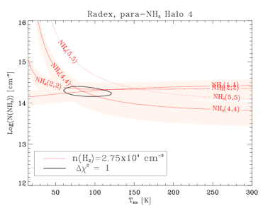
Figure 5: LVG diagram of NH₃ for Halo 4.

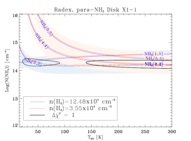
Figure 6: LVG diagram of NH₃ for Disk X1-1. The blue lines correspond to the low temperature regimen, and the red lines to the high temperature regimen.

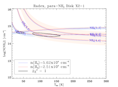
Figure 7: LVG diagram of NH₃ for Disk X2-1. The blue lines correspond to the low temperature regimen, and the red lines to the high temperature regimen.

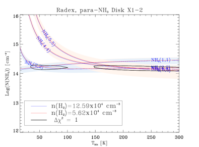
Figure 8: LVG diagram of NH₃ for Disk X1-2. The blue lines correspond to the low temperature regimen, and the red lines to the high temperature regimen.

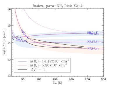
Figure 9: LVG diagram of NH₃ for Disk X2-2. The blue lines correspond to the low temperature regimen, and the red lines to the high temperature regimen.

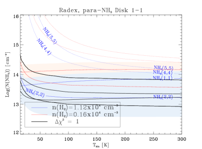
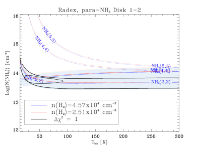
Figure 10: LVG diagrams of NH₃ for each velocity component of Disk 1. Top: $56.5\,{\rm km\,s}^{-1}$. Bottom: $72.4\,{\rm km\,s}^{-1}$. The blue lines correspond to the low temperature regimen, and the red lines to the high temperature regimen.

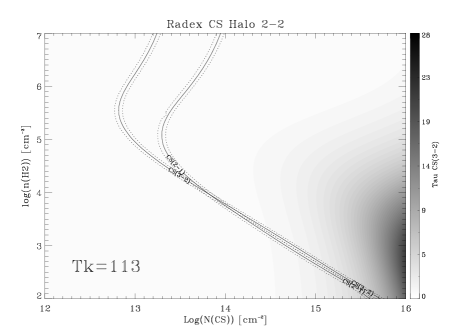
Figure 13: LVG diagrams of CS for each velocity component of Halo 2. Top:$-80\,{\rm km\,s}^{-1}$. Bottom: $-51.9\,{\rm km\,s}^{-1}$.

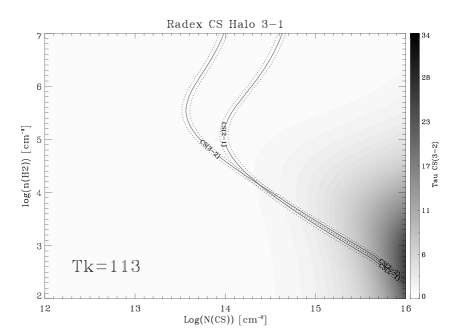
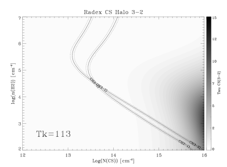
Figure 14: LVG diagrams of CS for each velocity component of Halo 3. Top: $-64.7\,{\rm km\,s}^{-1}$. Bottom: $-13.9\,{\rm km\,s}^{-1}$.

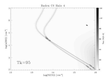
Figure 15: LVG diagrams of CS for Halo 4.

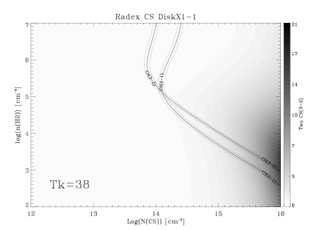
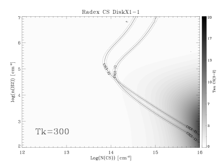
Figure 17: LVG diagrams of CS for each kinetic temperature regime of Disk X1-1.

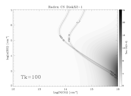
Figure 18: LVG diagrams of CS for each kinetic temperature regime of Disk X2-1

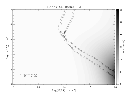
Figure 19: LVG diagrams of CS for each kinetic temperature regime of Disk X1-2

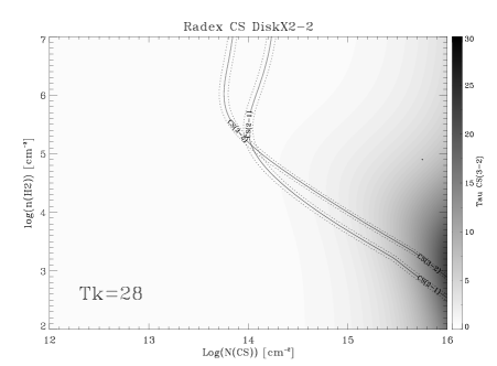
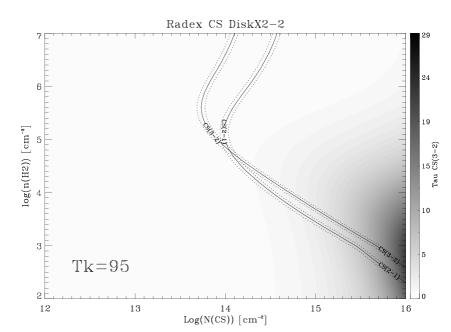
Figure 20: LVG diagrams of CS for each kinetic temperature regime of Disk X2-2

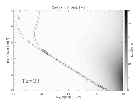
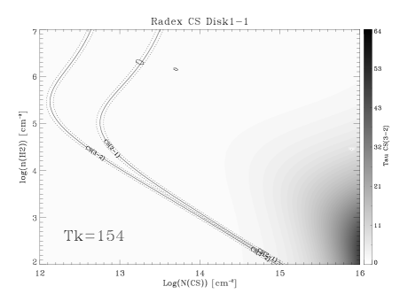
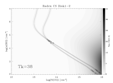
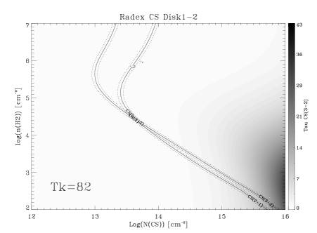
Figure 21: LVG diagrams of CS for each kinetic temperature regime, for each velocity component of Disk 1. Top: $56.8\,{\rm km\,s}^{-1}$. Bottom: $74.9\,{\rm km\,s}^{-1}$.