Population size bias in Diffusion Monte Carlo

Abstract

The size of the population of random walkers required to obtain converged estimates in DMC increases dramatically with system size. We illustrate this by comparing ground state energies of small clusters of parahydrogen (up to 48 molecules) computed by Diffusion Monte Carlo (DMC) and Path Integral Ground State (PIGS) techniques. We contend that the bias associated to a finite population of walkers is the most likely cause of quantitative numerical discrepancies between PIGS and DMC energy estimates reported in the literature, for this few-body Bose system. We discuss the viability of DMC as a general-purpose ground state technique, and argue that PIGS, and even finite temperature methods, enjoy more favorable scaling, and are therefore a superior option for systems of large size.

I INTRODUCTION

Quantum Monte Carlo (QMC) methods are widely utilized to compute accurate thermodynamics of quantum few-body systems. The best known, and arguably most popular such method, is the Diffusion Monte Carlo (DMC), which has been extensively adopted over the past three decades, especially in the context of electronic structure calculations for atoms and molecules Lester , but also in studies of light nuclei Pieper , as well as of small Bose clusters such as (⁴He)_N schmidt92 or (H₂)_N whaley . On the other hand, the Path Integral Ground State (PIGS) Ceperley1 ; Magro ; Roy and related methods baroni , have only relatively recently emerged as an interesting alternative to DMC. The most obvious advantage of PIGS over DMC is the straightforward, unbiased computation of ground state expectation values of quantities other than the energy, including off-diagonal correlations such as the one-body density matrix saverio ; holzmann ; carleo , not accessible within DMC. There is, however, another significant difference between the two methods, one that may have so far been overlooked and/or understated in the literature, namely that the results obtained by DMC are intrinsically biased by a necessarily finite population of random walkers. PIGS, on the other hand, is affected by no such limitation; we argue in this paper that this yields PIGS an edge over DMC, as systems of increasing number of particles are investigated. Specifically, we show quantitatively, using a simple test system, that the bias arising from a fixed finite population is a rapidly increasing function of the number $N$ of particles in the system (possibly leading to an exponential scaling of the computational cost); furthermore, for a given $N$ and for the typical numbers of random walkers commonly utilized, the bias can be both suprisingly large in magnitude, as well as difficult to control or remove, as the extrapolation of results obtained for different population sizes is not only very time-consuming, it can be quite problematic as well. We illustrate the above conclusions by carrying out a systematic comparison of ground state energy estimates yielded by DMC and PIGS, for a small cluster of parahydrogen (H₂) molecules, including between $N$=13 and $N$=48 molecules. We deem this a cogent test case, as a finite Bose cluster could be regarded as the paradigm physical system for which DMC ought to be applicable straightforwardly, almost as a “black box”.
The remainder of this manuscript is organized as follows: in the next section, we briefly review the basic differences between DMC and PIGS. Because both techniques are extensively discussed in the literature, we refer the reader to the appropriate references for a more in-depth illustration (see, for instance, Refs. Magro, ; umrigar, ). We then outline the model utilized in this work as a test case to perform calculations, and devote the bulk of this paper to a thorough presentation of the numerical results. We then discuss whether the bias due to a finite walker population may be the (main) cause of outstanding discrepancies between energy estimates for parahydrogen clusters reported in the literature, and offer our view on the importance of the population size bias on the scalability of DMC. On this point, we note that the hypothesis of an overall exponential scaling with $N$ of the computational resources needed for DMC, has already been put forward by others nemec .

II Methods

PIGS and DMC have the same theoretical basis; in both, the exact ground state of a quantum system is projected out of an initial trial state, by simulating on a computer its evolution in imaginary time. Consider for definiteness a system of $N$ identical particles of mass $m$; we assume for simplicity that the system obeys Bose statistics notesign .
The quantum-mechanical Hamiltonian $\hat{\cal H}$ of the system is

$$\hat{\cal H}=\hat{\cal H}_{\circ}+\hat{V}=-\lambda\sum_{i=1}^{N}\nabla^{2}_{i}+V(R)$$ (1)

where $\lambda={\hbar^{2}}/{2m}$, $R\equiv{\bf r}_{1}{\bf r}_{2}...{\bf r}_{N}$, are the positions of the $N$ particles, and $V(R)$ is the total potential energy of the system associated with the many-particle configuration $R$ (this is typically the sum of pairwise interactions, but can be more general). The exact ground state wave function $\Phi_{\circ}(R)$ can be formally obtained from an initial trial wave function $\Psi_{T}(R)$ as

$$\Phi_{\circ}(R)\propto{\rm lim}_{\beta\to\infty}\int dR^{\prime}\ G(R,R^{\prime},\beta)\ \Psi_{T}(R^{\prime})$$ (2)

where

$$G(R,R^{\prime},\beta)=\langle R|{\rm exp}[-\beta\hat{\cal H}]|R^{\prime}\rangle$$ (3)

is commonly referred to as the imaginary-time propagator. While Eq. (2) is formally exact, for a nontrivial many-body problem one does not normally have access to $G(R,R^{\prime},\beta)$. However, using one of several available schemes, it is possible to obtain approximations for $G$, whose accuracy increases as $\beta\to 0$; if $G_{\circ}(R,R^{\prime},\beta)$ is one such approximation, one can take advantage of the identity ${\rm exp}[-\beta\hat{H}]\equiv({\rm exp}[-\tau\hat{H}])^{M}$, with $\beta=M\tau$, and obtain $G(R,R^{\prime},\beta)$ as

$$G(R,R^{\prime},\beta)\approx\int\ \prod_{i=0}^{M-1}\ dR_{i}\ \biggl{\{}G_{\circ}(R_{i+1},R_{i},\tau)\biggr{\}}$$ (4)

where $R\equiv R_{0},\ R_{M}\equiv R^{\prime}$. Eq. (4) is exact in the limit $M\to\infty$ (i.e., $\tau\to 0$), which can be achieved in practice by extrapolating numerical results obtained with different values of $M$.

The difference between PIGS and DMC lies in how the above procedure is implemented numerically. In PIGS, one generates sequentially, on a computer, a large set $\{X^{p}\}$, $p=1,2,...,P$, of many-particle paths $X\equiv R_{0}R_{1}\ ...\ R_{2M}$ through configuration space. Each $R_{j}\equiv{\bf r}_{j1}{\bf r}_{j2}\ ...\ {\bf r}_{jN}$ is a point in 3$N$-dimensional space, representing positions of the $N$ particles in the system. These paths are statistically sampled, using the Metropolis algorithm, from a probability density

$${\cal P}(X)\propto\Psi_{T}(R_{0})\Psi_{T}(R_{2M})\ \biggl{\{}\prod_{i=0}^{2M-1}G_{\circ}(R_{i+1},R_{i},\tau)\biggr{\}}$$ (5)

It is a simple matter to show Ceperley1 ; Magro that in the limits $\tau\to 0$, $M\tau\to\infty$, $R_{M}$ is sampled from a probability density proportional to the square of the exact ground state wave function $\Phi_{\circ}(R)$, irrespective of the choice of $\Psi_{T}$ notey . One can therefore use the set $\{R_{M}^{p}\}$ of “midpoint” configurations $R_{M}$ of the statistically sampled paths, to compute ground state expectation values of thermodynamic quantities $F(R)$ that are diagonal in the position representation, simply as statistical averages, i.e.

$$\langle\Phi_{\circ}|\hat{F}(R)|\Phi_{\circ}\rangle\approx\frac{1}{P}\ \sum_{p=1}^{P}\ F(R_{M}^{p}),$$ (6)

an approximate equality, asymptotically exact in the $P\to\infty$ limit. The ground state expectation value of the energy can be obtained in several ways; it is particularly convenient to use the “mixed estimate”

$$\langle\Phi_{\circ}|\hat{H}|\Phi_{\circ}\rangle=\langle\Phi_{\circ}|\hat{H}|\Psi_{T}\rangle\approx\sum_{p=1}^{P}\ \frac{\hat{H}\Psi_{T}(R_{1}^{p})}{\Psi_{T}(R_{1}^{p})}$$ (7)

which provides an unbiased result for the Hamiltonian operator $\hat{H}$. Obviously, the total projection time $\beta\equiv M\tau$ remains finite. It is straightforward to prove that the energy estimate $E(\beta)$, corresponding to a finite value of $\beta$ is a strict upper bound on the exact ground state energy $E_{\circ}$, which is approached monotonically in the $\beta\to\infty$ limit as

$$E(\beta)-E_{\circ}\sim c\exp(-\beta\ \Delta E),$$ (8)

where $\Delta E$ is the energy gap between the ground state and the first excited state. By contrast, DMC implements the imaginary time evolution of the initial, trial state $\Psi_{T}$ by introducing an importance-sampling transformation of Eq. (2),

$$\Phi_{\circ}(R)\Psi_{G}(R)\propto$$

$${\rm lim}_{\beta\to\infty}\int dR^{\prime}\ {\tilde{G}}(R,R^{\prime},\beta)\ \Psi_{T}(R^{\prime})\Psi_{G}(R^{\prime}),$$ (9)

where $\Psi_{G}$ is a positive-definite guidance function and ${\tilde{G}}(R,R^{\prime},\beta)=\Psi_{G}(R)G(R,R^{\prime},\beta)/\Psi_{G}(R^{\prime})$. Hereafter, as almost invariably done for Bose systems, we take $\Psi_{T}=\Psi_{G}$. Eq. (II) is simulated by a guided, diffusive random walk through configuration space of a population of $N_{W}$ (ideally uncorrelated) walkers. Each walker performs successive transitions from its present configuration $R_{p}$ to a new one $R_{n}$, sampled from a diffusive probabilistic kernel contained in ${\tilde{G}}_{\circ}(R_{n},R_{p},\tau)$, with the addition of a drifting term which depends on $\Psi_{T}$. The aim of such a drifting term is allowing for importance sampling of the configurations, normally expected to reduce considerably the variance of the estimates. There is no importance sampling in PIGS, on the other hand Roy ; reatto . A crucial feature of DMC is the fact that walkers, along the random walk, accumulate weights proportional to ${\rm exp}[-\int d\tau E_{L}(\Psi_{T}(R))\tau)]$, where $E_{L}(\Psi_{T}(R))\equiv\hat{\cal H}\Psi_{T}(R)/\Psi_{T}(R)$ is the local energy given by the trial wave function at the configuration $R$, visited at imaginary time $\tau$ by a given walker. Typically, weights fluctuate considerably, both along the random walks, as well as within the population at any given time. Therefore, it proves convenient to reconfigure the population, every now and then during the calculation, so that walkers whose weights have become negligibly small are discarded, and copies are made of walkers whose weights are larger. This reconfiguration, known as branching, is done in such a way that fluctuations in the weights of individual walkers remain limited. In addition, control must be exerted in order to limit fluctuations in the population size (or total weight). Here too, it is possible to show that in the limit of long projecion time the population of walkers will sample a distribution of configurations proportional to $\Phi_{\circ}(R)\Psi_{T}(R)$, which can then be used to evaluate the exact ground state energy. The main advantage of this computational strategy, at least in principle, is that the projection time can be made very large with little computational effort. On the other hand, a bias is introduced in the procedure, as one must necessarily work with a finite population of walkers. In order for the algorithm to be exact, extrapolation to infinite population size must be carried out (see, for instance, Ref. umrigar, for details). There has been surprisingly little work aimed at establishing the magnitude of the finite population size bias on the computed expectation values, but some calculations have shown that it can be significant, particularly when trying to estimate expectation values of operators that do not commute with the Hamiltonian runge92 ; calandra ; ceperleylast . On general grounds, one can expect the bias to depend on the accuracy of the guiding wave function $\Psi_{T}$; if, hypothetically, the exact ground state wave function were known, then a single walker would suffice, as branching would disappear and the DMC calculation would reduce to a variational one, as expected. On the other hand, the less accurate $\Psi_{T}$, the more significant the fluctuations of the local energy associated to individual walkers, and with those the more important the effect of branching, from which the need for a larger population size ensues. Within PIGS there is no such bias, as there is no population and no branching.

III Model and calculations

Our physical system of interest, for which we present all the numerical results discussed here, is a self-bound cluster of $N$ parahydrogen molecules, regarded as point particles, moving in three dimensions. This system has been the subject of much theoretical investigation over the past few years, as it is believed to display an interesting interplay of classical and quantum-mechanical physical effects holland . Clusters of parahydrogen of less than 20 molecules are liquidlike and superfluid at low $T$; if the number of molecules is between 20 and 40, clusters can “quantum melt” at low temperature i.e., go from a solidlike arrangements, with molecules sitting at preferred sites, to a superfluid one, in which they are essentially delocalized throughout the cluster mezzacapo ; mezzacapo1 . Moreover, some specific “supersolid” clusters, superfluid and solid behaviours appear to coexist in the $T\to 0$ limit supersolid . An interesting issue is whether there exist clusters of specific sizes (also referred to as “magic numbers”) that enjoy enhanced stability over others. This has been investigated in a number of works by computation of the total ground state energy $E(N)$, as a function of cluster size $N$, and by looking for isolated peaks of the chemical potential $\mu(N)$, defined as

$$\mu(N)=E(N-1)-E(N)$$ (10)

Clearly, the precise identification of magic clusters requires a sufficiently accurate determination of $E(N)$, which is an extensive quantity. At present, there exist outstanding discrepancies between different ground state results obtained by DMC guardiola ; sola , PIGS cuervo , as well as by extrapolating to $T=0$ results at finite temperature holland . This point is discussed in detail below, where we argue that the population size bias in DMC is likely at the root of such a discrepancy between different calculations, at least for the largest size clusters. The quantum-mechanical many-body Hamiltonian is given by Eq. (1), with $\lambda=12.031$ KŲ and the following choice for the potential energy $V(R)$:

$$V(R)=\sum_{i<j}v(r_{ij})$$ (11)

Here, $v$ is the potential describing the interaction between two hydrogen molecules, only depending on their relative distance. It should be made clear at the outset that such a simple model potential is not the most accurate choice that one could make; three-body terms are known to be quantitatively important. However, since the aim of this paper is mostly methodological, we limit ourselves to the use of a pair potential, and select that by Silvera and Goldman sg , for consistency with existing calculations against which we are interested in comparing our results. We have computed ground state energies of clusters of size ranging between $N$=13 and $N$=48, using both PIGS as well as DMC.

III.1 PIGS

Our PIGS calculations are based on a trial wave function of the Jastrow type

$$\Psi_{P}(R)=\prod_{i<j}\ {\rm exp}[-u(r_{ij})]$$ (12)

where $r_{ij}\equiv|{\bf r}_{i}-{\bf r}_{j}|$, and with $u(r)=\alpha/r^{5}$, $\alpha$ being a variational parameter whose value was set to 375 Å⁵ for all clusters studied here. This wave function is the same employed in previous studies based on PIGS cuervo , albeit with a different value of the parameter $\alpha$. It is not meant to describe a finite self-bound system, in that it only includes short-range correlations arising from the repulsive core of the intermolecular potential. A variational calculation based on such a trial wave function yields an unbound cluster, i.e., $E(N)=0$. One of the most important aspects of PIGS is precisely its ability to extract the correct physics even if the initial trial wave function is chosen less than optimally; for example, in Ref. reatto it is shown that an accurate ground state energy estimate for solid helium can be obtained by PIGS even on setting the trial wave function equal to a constant. This is in stark contrast to DMC, for which an appropriate choice for $\Psi_{T}$ often proves crucial to the accuracy and reliability of the calculation.
In this work, the same approximation for $G(R,R^{\prime},\tau)$ utilized in Refs. Roy ; cuervo was chosen, namely:

$$G_{\circ}(R,R^{\prime},\tau)=G_{F}(R,R^{\prime},\tau)\ {\rm exp}\biggl{[}-\frac{2\tau\tilde{V}(R)}{3}\biggr{]}$$ (13)

where $G_{F}(R,R^{\prime},\tau)$ is the analytically known propagator for a system of non-interacting particles and

$$\tilde{V}(R_{j})=2V(R_{j})+\frac{\tau^{2}\hbar^{2}}{6m}\sum_{i=1}^{N}(\nabla_{i}{V}(R_{j}))^{2}$$ (14)

if $j$ is odd, whereas $\tilde{V}(R_{j})=V(R_{j})$ is $j$ is even. It is $G(R,R^{\prime},\tau)=G_{\circ}(R,R^{\prime},\tau)+{\cal O}(\tau^{5})$. The path sampling techniques are the same described in Ref. Roy .

III.2 DMC

For the DMC calculations we adopt the same trial function used in Ref. sola , $\Psi_{D1}(R)=\prod_{i<j}{\rm exp}[-w(r_{ij})]$, where the pair pseudopotential $w(r)=\beta/r^{5}+br/N$ differs from $u(r)$ of Eq. (12) for the need to include a linear term which prevents molecules from evaporating; the variational parameters are sola $\beta=294$ Å⁵ and $b=2.79$ Å^-1. We also consider a much better trial function $\Psi_{D2}(R)$ with a more flexible pair pseudopotential and a three-body correlation of the standard form skl , both optimized euler for each cluster size. For $N=48$, the variance of the local energy of $\Psi_{D2}$ is smaller than that of $\Psi_{D1}$ by over an order of magnitude. Significantly better trial functions can only be obtained by including four- and five-body terms nightingale , but this route seems to be viable only for very small systems. The details of the DMC simulations are essentially those described in Ref. umrigar , notably we utilize the standard approximation for the propagator, supplemented with the well-known “rejection” scheme, which has been shown to afford convergence of the numerical estimates with a significantly greater time step than would be otherwise required. We only use a slightly different translation of weights into multiplicity during the branching reconfiguration. Before we discuss the results, a point must be made clear, namely that our purpose here is to carry out an unambiguous, unbiased comparison of energy estimates obtained by DMC and PIGS. Because we are considering a Bose system, for which the ground state wave function is positive-definite, the numerical results given by the two algorithms are expected to coincide, within statistical uncertainties, once extrapolations to infinite projection time for PIGS, infinite size of the population sample for DMC, and zero time step for both are carried out. Implementation details of either method, such as the approximation adopted for the short-time propagator or the choice of the moves in the random walk, only affect the efficiency of the calculations, and are of no particular concern here. On the other hand the population bias of DMC, which is the focus of our study, depends on the quality of the trial function (which cannot be arbitrarily improved in general) to such an extent that the extrapolation to infinite number of walkers can be problematic or even unfeasible in practice.

IV RESULTS

In order to establish our main finding, we begin by illustrating results of calculations of ground state energetics for the largest cluster studied here, comprising $N$=48 parahydrogen molecules. Specifically, we compare PIGS and DMC results.
Figure 1 shows estimates of the ground state energy per parahydrogen molecule $e\equiv E/N$ obtained by PIGS with a total projection time $\beta$=1 K^-1, and with different values of the time step $\tau$. A fit to the data based on the expression $e(\beta,\tau=0)=e(\beta,\tau)+c\tau^{4}$, justified by the use of the propagator (13), yields a value extrapolated to $\tau=0$ equal to $e(\beta=1$ K${}^{-1},\tau=0)=-38.14(1)$ K.

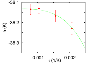
Figure 1: (Color online). Estimates of the ground state energy per particle for a cluster of 48 parahydrogen molecules, computed by PIGS as explained in the text, for varying values of the time step $\tau$ (in K^-1). The total projection time is $\beta=$1 K^-1. The dashed line shows a quartic fit to the data, extrapolating to a $\tau=0$ limit of -38.14(1) K.

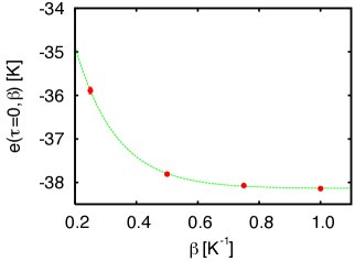
Figure 2: (Color online). Extrapolation to the $\beta\to\infty$ limit of estimates of the ground state energy per particle for a cluster of 48 parahydrogen molecules, computed by PIGS as explained in the text, for varying values of the projection time $\beta$. Estimates shown are extrapolated to the $\tau\to 0$ limit. Dashed line is the fitting curve described in the text.

As mentioned above, an estimate for $e(\beta=\infty,\tau=0)$ can be obtained by extrapolating results obtained with different projection times curiosity . The result is shown in Figure 2. The asymptotic value is indistinguishable, within statistical errors, from that at $\beta=1$ K^-1. Our energy estimate is slightly higher than that offered in Ref. cuervo , namely $-38.22(3)$ K, for a projection time $\beta=0.8$ K^-1 and with a time step $\tau$ = $1.5625\times 10^{-3}$ K^-1. For the same time step, our estimate is $-38.17(2)$ K (see Figure 1), compatible with that of Ref. cuervo if statistical uncertainties are taken into account noteourtimestep . On the other hand, it is surprisingly almost 1 K below the most recent DMC estimate for this cluster, namely $-37.28(3)$ K, by Sola and Boronat sola . Such a discrepancy can hardly be regarded as “negligible”, considering that the value of the chemical potential $\mu(N)$ (Eq. 10), used to assess cluster stability, is computed by subtracting two extensive energy values, i.e., associated to whole clusters. For instance, a systematic error of the order of 0.9 K per molecule results into one on the total energy of the $N=48$ cluster of approximately 45 K, which is very close to the value of $\mu$ quoted in Ref. sola, for this cluster.
In order to shed light on this worrisome disagreement between numerical data advertised as “exact”, we have performed DMC calculations for the same cluster, as explained above. All the results presented so far are calculated with a time step of $2.0\times 10^{-4}$ K^-1. We find that the time step error on the energy per particles is similar for all clusters, in the range of sizes considered here. It does depend on the trial function, however. Our estimates are -0.07 K for $\Psi_{D1}$ and less than 0.01 K for $\Psi_{D2}$.

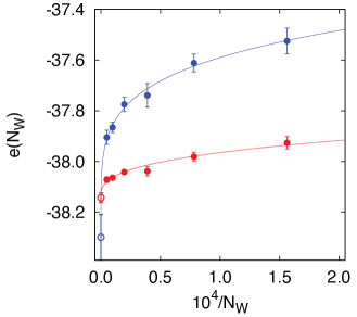
Figure 3: (Color online). Ground state energy per particle for a cluster of 48 parahydrogen molecules as a function of the number of walkers $N_{W}$, computed by DMC using two different trial functions: $\Psi_{D1}$ (diamonds, blue online) and $\Psi_{D2}$ (circles, red online). The lines are power law fits to the data, and the open symbols show the extrapolated values at $1/N_{W}=0$. The time step utilized here is 0.0002 (in K^-1).

Figure 3 shows the ground state energy per particle for a cluster of 48 parahydrogen molecules as a function of the number of walkers, calculated with the trial functions $\Psi_{D1}$ and $\Psi_{D2}$ of Sec. III.2. If the walkers were uncorrelated, the population bias would vanish as $1/N_{W}$ umrigar . This is clearly not the case: for both trial functions, we can fit data obtained with $N_{W}$ between 200 and 200,000 (not all of this range is shown in Figure 3) with the expression $e(N_{W})=e(\infty)+cN_{w}^{k}$, and the optimal value of the exponent is 0.342 for the “good” trial function $\Psi_{D2}$, and as low as 0.202 for the “poor” trial function $\Psi_{D1}$, the reduced $\chi^{2}$ being smaller than 1 in both cases.
There are several things to note here. First and foremost, the result $e=-37.278\pm 0.028$ reported in Ref. sola, for $N=48$, allegedly based on data “analyzed to reduce any sistematic bias to the level of statistical noise”, is outside the scale of the figure. The DMC energies of Ref. sola, are systematically higher than those reported in Ref. cuervo, , the difference increasing (non-monotonically) with $N$; we find it to be greatest ($\sim 0.9$ K) at $N$=48, while it is of the order of 0.2 K per molecule for $N$=30, and 0.4 K per molecule at $N$=40.
In Ref. guardiola, , which reports DMC energy estimates (essentially identical with those of Ref. sola, ) for clusters of size up to $N$=40, authors observe a “marked” effect of population size, on performing calculations for $N_{W}$ ranging from 500 to 2,000, suggesting nevertheless that its overall effect on the chemical potential might be negligible, presumably due to some expected (fortunate) compensation of error.
Indeed, our DMC values are similar to those of Refs. sola, ; guardiola, , when we take $N_{W}\sim 1500$; the problem is that the small slope of the $e(N_{W})$ curve around such a value of $N_{W}$ is highly deceiving, as the slope actually appears to diverge, as $1/N_{W}\to 0$, as clearly shown by data in Figure 3. Therefore, not only is extrapolation of results which depend so dramatically on the number of walkers clearly problematic – one can be easily led to believe incorrectly that convergence with respect to $N_{W}$ has been reached, by focusing on relatively narrow a range of $N_{W}$, as in Ref. guardiola, (it does not help if discrepancies with published results by others are simply ignored). The extrapolated value agrees, as it should, with the PIGS result (within two standard deviations, for $\Psi_{D2}$), but the amount of computer time needed to reach a given statistical accuracy is much larger for DMC than for PIGS.
For $N=23$ the population bias is still definitely not linear in $1/N_{W}$, but its magnitude is much smaller than for $N=48$; deviations from the linear behavior become hard to detect for $N=13$. We can define the number of walkers ${\bar{N}_{W}}$ needed to observe convergence of the energy to a precision $\epsilon$ via the relation $e({\bar{N}_{W}})-e(\infty)=\epsilon$. For $\epsilon=0.01$ K we find ${\bar{N}_{W}}=5000$ for $N=13$ and as much as ${\bar{N}_{W}}=100$ millions for $N=48$ if we use $\Psi_{D2}$. A sensible estimate for $N=48$ using $\Psi_{D1}$ is not even possible from our simulations, which in this case, even using up to 200,000 walkers, still leave a large uncertainty in the best-fit exponent of $e(N_{W})$. In terms of the comparison between the DMC sola ; guardiola and the PIGS cuervo results (see Table 1), which initially motivated this work, the dependence of the popolation bias on the system size parallels and presumably explains the similar dependence in the observed discrepancies.

$N$	DMCsola	DMC	PIGS
13	$-20.952(16)$	$-20.98(1)$	$-21.02(1)$
23	$-28.111(12)$	$-28.15(1)$	$-28.16(1)$
36	$-33.804(19)$	$-34.09(2)$	$-34.13(1)$
48	$-37.278(28)$	$-38.15(2)$	$-38.14(1)$

Table 1: Ground state energy per molecule (in K) for different parahydrogen clusters, computed by DMC (Ref. sola, and this work) and PIGS. PIGS estimates are extrapolaed to the $\tau\to 0$ limit, for a total projection time $\beta=1$ K^-1. DMC estimates obtained in this work are extrapolated to the $1/N_{W}\to 0$ limit as explained in the text. Statistical errors, in parentheses, are on the last digit(s).

V Discussion

Although the results shown above illustrate rather clearly that the bias arising from the control of the population is significant, it could be argued that the use of a more accurate trial wave function (e.g., $\Psi_{D2}$ instead of $\Psi_{D1}$ in the case shown in Figure 1), considerably improves the convergence, and therefore it is unclear whether the problem should be ascribed to a finite population, or rather to a poor choice of $\Psi_{T}$. As it turns out, although a superior trial wave function can indeed alleviate the problem of finite population bias, this should not induce much optimism on the scalability of DMC in general. For, the behavior illustrated in Figure 3 is ultimately due to statistical correlation between walkers, in turn induced by large fluctuations of the branching term $\exp(-\tau E_{L}(R))$. Since $E_{L}$ is an extensive quantity, one can expect –and does indeed observe nemec – an extremely poor asymptotic scaling of the efficiency of DMC with the system size. For molecular hydrogen, this problem compounds with a relatively low quality of the trial function; the strength of the interparticle potential makes it difficult to devise and use much more accurate trial wave functions than $\Psi_{D2}$. As a result, $N=48$ – a very modest size for a boson system vermer – turns out to be already a demanding calculation.
On this point, it is interesting to note that, in a previous study Roy , a comparison of ground state energy estimates for bulk liquid ⁴He obtained with PIGS and DMC, found that PIGS yielded consistently lower results, and that the difference between PIGS and DMC results increases with density. The suggestion was already made back then that the use of a finite population in DMC, comprising only a few hundred walkers in those DMC calculations, seems very likely to be the cause of the discrepancy.

Figure 4: Ground state energy per particle for a cluster of 48 parahydrogen molecules as a function of $T_{P}$, computed by DMC using the $\Psi_{D2}$ trial function with $N_{W}=12800$. Error bars are only shown for a few points. The horizontal line is the extrapolated value at $1/N_{W}=0$ from Figure 3. The time step utilized here is 0.0002 (in K^-1).

It should also be mentioned that there exists an alternative procedure, one that in principle could remove the bias due to a finite population of walkers in DMC without requiring an extrapolation with $N_{W}$. One can carry out the DMC simulation with a single target value of $N_{W}$ and store the renormalization factors $f_{i}$ of the population size along the simulation umrigar , with $i$ a time index. The bias would be eliminated by accumulating weighted averages, the weight being defined for each configuration as the inverse of the product of all factors $f_{i}$ from the beginning of the simulation up to the current time.
While in principle this procedure completely undoes the effect of the population control, in practice it leads to unacceptably large variance. Thus, one keeps in the weighted averages only the product of the last $K_{P}$ factors $f_{i}$, and seeks convergence of the results by increasing the “correction time” $T_{P}=K_{P}\tau$. However, one is bound to face severe efficiency problems whenever the population size bias is strong. Figure 4 illustrates an attempt at correcting the population size bias for the ground state energy of a cluster of 48 parahydrogen molecules calculated with 12800 walkers. From the biased value at $T_{P}=0$ the energy is expected to converge for large times to the exact value (the extrapolation of Figure 3, shown in Figure 4 by the horizontal line). However no convincing evidence of convergence can be detected before the statistical error grows as large as the bias itself, despite this simulation being 8 times longer than that performed for the single point at $N_{W}=12800$ of Figure 3.
In conclusion, we have presented numerical evidence to the effect that the bias arising from a finite population size in DMC calculations is the most likely cause of discrepancies reported in the literature between ground state energy estimates for Bose systems obtained with DMC and Metropolis-based methods such as PIGS. Although a complete removal of the bias (whose magnitude appears to have been generally underestimated, or in any case not fully appreciated) is possible in principle, the computational resources required grow significantly with system size. In fact, although the system sizes for which we are presenting data in this work are too small to make that conclusion, they are strongly suggestive of exponential scaling. Obviously, although we have illustrated quantitatively this conclusion on a Bose system, it applies equally to fermions, there being nothing in the argument expounded here that depends on quantum statistics. If anything, there are reasons to expect that the use of the popular fixed-node approximation to circumvent the sign problem may conceivably worsen the problem of fluctuating local energy, which is at the root of the population bias. Thus, while the choice between the two methods has been so far largely regarded as one of “personal taste”, path integral methods, requiring no walker population, may prove a better choice for systems of large size, how large depending on the quality of the trial function.
Finite temperature methods such as Path Integral Monte Carlo, which do not require a population of walkers, also do not suffer from the kind of bias discussed in this work, that affects instead any population-based procedure such as GFMC (including for lattice Hamiltonians) and DMC. Thus, although one may naively think that ground state methods would necessarily be better suited for $T$=0 calculations, PIMC may in fact also prove a better option than DMC in some cases, given the significance of the population size bias. It is worth mentioning that for the specific physical system discussed her, PIMC yields estimates in the $T\to 0$ limit consistent with those furnished by PIGS holland ; mezzacapo ; mezzacapo1 .

References

- (1) See, for instance, D. Y. Zubarev, B. M. Austin and W. A. Lester Jr. in Practical Quantum Chemistry I, J. Leszczynski and M. K. Shukla eds., (Springer-Verlag, Berlin, 2012), and references therein.
- (2) See, for instance, S. C. Pieper, Nucl. Phys. A751, 516 (2005), and references therein.
- (3) See, for instance, K. E. Schmidt and D. M. Ceperley in The Monte Carlo Method in Condensed Matter Physics, K. Binder editor, Topics in Applied Physics (Springer-Verlag, Berlin, 1992), Vol. 71, and references therein.
- (4) M. McMahon and K. B. Whaley, Chem. Phys. 182, 119 (1994).
- (5) D. M. Ceperley, Rev. Mod. Phys. 67, 279 (1995).
- (6) A. Sarsa, K. E. Schmidt, and W. R. Magro, J. Chem. Phys. 113, 1366 (2000).
- (7) J. E. Cuervo, P.-N. Roy and M. Boninsegni, J. Chem. Phys. 122, 114504 (2005).
- (8) S. Baroni and S. Moroni, Phys. Rev. Lett. 82, 4745 (1999).
- (9) S. Moroni and M. Boninsegni, J. Low Temp. Phys. 136, 129 (2004).
- (10) M. Holzmann, B. Bernu, C. Pierleoni, J. McMinis, D. M. Ceperley, V. Olevano and L. Delle Site, Phys. Rev. Lett. 107, 110402 (2011).
- (11) G. Carleo, S. Moroni, F. Becca, S. Baroni, Phys. Rev. E 82, 046710 (2010).
- (12) C. J. Umrigar, M. P. Nightingale, and K. J. Runge J. Chem. Phys. 99, 2865 (1993).
- (13) N. Nemec, Phys. Rev. B 81, 035119 (2010).
- (14) Population bias affects DMC regardless of quantum statistics, and there are no obvious reasons to expect it to be worse for either Fermi or Bose systems. Of course, QMC simulations of Fermi systems are also affected by the “sign problem”, but this is a separate issue, unrelated to what we discuss in this paper. We therefore restrict our discussion to Bose statistics for convenience and simplicity.
- (15) Strictly speaking, is required to be non-orthogonal to the true ground state wave function. For a Bose system (such as condensed 4He) this is not a problem, as the ground state wave function can always be chosen real and positive, and therefore any positive-definite function satisfies the non-orthogonality requirement. That be non-negative is of course also crucial in order for (5) to be treated as a probability.
- (16) M. Rossi, M. Nava, L. Reatto, and D. E. Galli, J. Chem. Phys. 131, 154108 (2009).
- (17) M. Calandra Bonaura and S. Sorella, Phys. Rev. B 57, 11446 (1998).
- (18) K. J. Runge, Phys. Rev. B 45, 7229 (1992).
- (19) J. T. Krogel and D. M. Ceperley, Population Control Bias with applications to Parallel Diffusion Monte Carlo, Advances in Quantum Monte Carlo, eds. S. Tanaka, S. Rothstein, W.A. Lester Jr., ACS Symposium Series Vol. 1094, 13 (2012).
- (20) F. Mezzacapo and M. Boninsegni, J. Phys. CM 21, 164205 (2009).
- (21) F. Mezzacapo and M. Boninsegni, Phys. Rev. Lett. 96, 045301 (2006).
- (22) F. Mezzacapo and M. Boninsegni, Phys. Rev. A 75, 033201 (2007).
- (23) F. Mezzacapo and M. Boninsegni, J. Phys. Chem. A 115, 6831 (2011).
- (24) R. Guardiola and J. Navarro, Cent. Eur. J. Phys. 6, 33 (2008).
- (25) E. Sola and J. Boronat, J. Phys. Chem. A 115, 7071 (2011).
- (26) J. E. Cuervo and P.-N. Roy, J. Chem. Phys. 128, 224509 (2008).
- (27) I. Silvera and V. V. Goldman, J. Chem. Phys. 69, 4209 (1978).
- (28) K. Schmidt, M. H. Kalos, and Michael A. Lee, Phys. Rev. Lett. 45, 573 (1980).
- (29) S. Moroni, S. Fantoni, and G. Senatore, Phys. Rev. B 52, 13547 (1995).
- (30) A. Mushinski and M. P. Nightingale, J. Chem. Phys. 101, 8831 (1994).
- (31) This corresponds to the “transient estimate” procedure utilized for calculations affected by a “sign” problem, in which statistical errors increase exponentially with projection time. See, for instance, M. Boninsegni and E. Manousakis, Phys. Rev. B 47, 11897 (1993).
- (32) The values of the energy per molecule published in Ref. cuervo appear to be affected by a systematic downward shift worth between 0.05 and 0.1 K, due to time step error. We have established that, within PIGS, the largest time step for which estimates are indistinguishable from those extrapolated to the limit, within our quoted statistical uncertainties, is approximately K-1.
- (33) M. Holzmann and W. Krauth, Phys. Rev. Lett. 100 190402 (2008).