Non-Gaussianity of a single scalar field in general covariant Hořava-Lifshitz gravity

Abstract

In this paper, we study non-Gaussianity generated by a single scalar field in slow-roll inflation in the framework of the non-relativistic general covariant Hořava-Lifshitz theory of gravity with the projectability condition and an arbitrary coupling constant $\lambda$, where $\lambda$ characterizes the deviation of the theory from general relativity (GR) in the infrared. We find that the leading effect of self-interaction, in contrary to the case of minimal scenario of GR, is in general of the order $\hat{\alpha}_{n}\epsilon^{3/2}$, where $\epsilon$ is a slow-roll parameter, and $\hat{\alpha}_{n}\;(n=3,5)$ are the dimensionless coupling coefficients of the six-order operators of the Lifshitz scalar, and have no contributions to power spectra and indices of both scalar and tensor. The bispectrum, comparing with the standard one given in GR, is enhanced, and gives rise to a large value of the nonlinearity parameter $f_{\text{NL}}$. We study how the modified dispersion relation with high order moment terms affects the evaluation of the mode function and in turn the bispectrum, and show explicitly that the mode function takes various asymptotic forms during different periods of its evolution. In particular, we find that it is in general of superpositions of oscillatory functions, instead of plane waves like in the minimal scenario of GR. This results in a large enhancement of the folded shape in the bispectrum.

I Introduction

The Hořava-Lifshitz (HL) theory of quantum gravity, proposed recently by Hořava Horava , motivated by the Lifshitz scalar field theory in solid state physics Lifshitz , has attracted a great deal of attention, due to its several remarkable features in cosmology as well as some challenging questions, such as instability, ghost, strong coupling, and different speeds reviews . To resolve these questions, various models have been proposed, along two fundamentally different lines, one with the projectability condition SVW ; HMT ; WW ; dS ; HW ,

$$N=N(t),$$ (1.1)

and the other without it BPS ; ZWWS , where $N$ denotes the lapse function in the Arnowitt, Deser and Misner decompositions ADM . In particular, Hořava and Melby-Thompson (HMT) proposed to enlarge the foliation-preserving diffeomorphisms of the original model,

$$\delta{t}=-f(t),\;\;\;\delta{x}^{i}=-\zeta^{i}(t,{\bf x}),$$ (1.2)

often denoted by Diff($M,\;{\cal{F}}$), to include a local U(1) symmetry, so that the reformulated theory has the symmetry HMT ,

$$U(1)\ltimes{\mbox{Diff}}(M,\;{\cal{F}}).$$ (1.3)

With such an enlarged symmetry, the spin-0 gravitons, which appear in the original model of the HL theory Horava , are eliminated HMT ; WW , and as a result, all the problems related to them, including instability, ghost, and strong coupling, are resolved automatically. This was initially done with $\lambda=1$, where $\lambda$ characterizes the deviation of the theory from general relativity (GR) in the infrared, as one can see from Eqs.(2.1) and (II) given below. Soon, it was generalized to the case with any $\lambda$ dS , in which it was shown that the spin-0 gravitons are also eliminated HW ; dS , so that the above mentioned problems are resolved in the gravitational sector. In the matter sector, the strong coupling problem, first noted in HW , can be solved by introducing a mass $M_{*}$ so that $M_{*}<\Lambda_{\omega}$, where $M_{*}$ denotes the suppression energy of high order operators, and $\Lambda_{\omega}$ the would-be energy scale, above which matter becomes strongly coupled LWWZ , similar to the non-projectability case without the enlarged symmetry BPSb . The consistence of this model with solar system tests was investigated recently LMW , and found that it is consistent with all such tests, provided that the gauge field and Newtonian prepotential are part of the metric, as proposed originally by HMT HMT .

In this paper, we shall work within the HMT framework of the HL theory with the projectability condition HMT ; WW ; dS ; HW . For the current status of the models proposed in SVW ; BPS ; ZWWS , we refer readers to LMW .

Since the HL theory differs from GR significantly in high energies, in this paper we study another important issue - the primordial non-Gaussianity in the HL theory. Such a problem was studied previously, one without the projectability condition Gao , and the other with it Shinji-II but in the curvaton scenario Curvaton , and many interesting results were obtained. However, our study presented in this paper are different from these at least in two aspects: (i) we shall study the problem in the framework of the non-relativistic general covariant Hořava-Lifshitz theory of gravity with the projectability condition HMT ; WW ; dS ; HW , as mentioned above, in which the degree of gauge freedom is the same as that in GR; and (ii) we shall investigate the problem in the inflationary scenario for a single scalar field with slow-roll conditions . Because of these differences, our results are also significantly different from theirs.

To study non-Gauusianity, various techniques have been developed. In particular, the in-in formalism, developed initially by Schwinger some decades ago Schwinger , becomes standard, after it was first explored by Madalcena in his pioneer work Madalcena in calculating the high-order correlators for cosmological perturbations, and then further developed by Weinberg in his seminal paper Weinberg05 . For reviews, see Koyama ; Contractions . In this paper, we will follow this approach.

Non-Gauusianities have attracted lot of attention recently and been studied extensively in various models Koyama ; Contractions , mainly because they could be well within the range of detection of the current Planck satellite Planck and the forthcoming experiments, such as the CMBPol mission CMBPol . Among various models, the one with a canonically coupled single scalar field in the framework of GR, though the simplest, gives elegant predictions and fits extremely well with current observations COBE . It predicts that the quantum fluctuations, which are responsible for generating the primordial perturbations and in turn the anisotropies in CMB and inhomogeneity in the large scale structure, are largely Gaussian. The effect of the non-linearity in the primordial perturbations is an order smaller than that of the power spectrum and is beyond our current detectabilities.

However, Holman and Tolley recently argued that, while a change in high energy physics during or before inflation gives mild modifications to the power spectrum and index, the non-Gaussianity, evaluated by higher order correlation functions of the perturbations, is much more sensitive to the new physics in the ultraviolet (UV) Holman . Therefore, it is very interesting to study the non-Gaussianity in the scalar primordial perturbations of the HL theory, where the dispersion relations are quite different from the standard one.

The rest of the paper is organized as follows. In Section II we give a brief review of the non-relativistic general covariant Hořava-Lifshitz theory of gravity with the projectability condition and an arbitrary coupling constant $\lambda$. The self-interaction Hamiltonian and the leading order terms are analyzed in Section III. Section IV discusses the modified dispersion relation and its effect on the mode function and the shapes of bispectrum. We also compare our results with those presented in Shinji-II . Finally, in Section V we summarize our results and the assumptions made along the way of analysis. Three appendices are also included, where in Appendix A the linear perturbations and the corresponding field equations are presented, while in Appendix B, the cubic part of the total action is calculated, and given explicitly. In Appendix C, the matching across the boundaries among the three different regions of the time revolution of the mode function [cf. Fig. 1] are given.

II General covariant HL gravity with projectability condition

The action of the general covariant HL theory of gravity with the projectability condition can be written as HMT ; WW ; dS ; HW ,

$$S = \frac{1}{16\pi G}\int dtd^{3}xN\sqrt{g}\Big{(}{\cal{L}}_{K}-{\cal{L}}_{{V}}+{\cal{L}}_{{\varphi}}+{\cal{L}}_{{A}}+{\cal{L}}_{{\lambda}}\Big{)}$$ (2.1)

$$~{}~{}~{}~{}+\int dtd^{3}xN\sqrt{g}{\cal{L}}_{M},$$

where $g={\rm det}(g_{ij})$, $G$ is the Newtonian constant, and

$${\cal{L}}_{K} = K_{ij}K^{ij}-\lambda K^{2},$$

$${\cal{L}}_{{V}} = \zeta^{2}g_{0}+g_{1}R+\frac{1}{\zeta^{2}}\left(g_{2}R^{2}+g_{3}R_{ij}R^{ij}\right)$$

$$+\frac{1}{\zeta^{4}}\left(g_{4}R^{3}+g_{5}R\;R_{ij}R^{ij}+g_{6}R^{i}_{j}R^{j}_{k}R^{k}_{i}\right)$$

$$+\frac{1}{\zeta^{4}}\left[g_{7}R\Delta R+g_{8}\left(\nabla_{i}R_{jk}\right)\left(\nabla^{i}R^{jk}\right)\right],$$

$${\cal{L}}_{\varphi} = \varphi{\cal{G}}^{ij}\Big{(}2K_{ij}+\nabla_{i}\nabla_{j}\varphi\Big{)},$$

$${\cal{L}}_{A} = \frac{A}{N}\Big{(}2\Lambda_{g}-R\Big{)},$$

$${\cal{L}}_{\lambda} = \big{(}1-\lambda\big{)}\Big{[}\big{(}\Delta\varphi\big{)}^{2}+2K\Delta\varphi\Big{]}.$$ (2.2)

Here $\Delta\equiv g^{ij}\nabla_{i}\nabla_{j}$, $\Lambda_{g}$ is a coupling constant, the Ricci and Riemann tensors $R_{ij}$ and $R^{i}_{jkl}$ all refer to the 3-metric $g_{ij}$, and

$$K_{ij} = \frac{1}{2N}\left(-\dot{g}_{ij}+\nabla_{i}N_{j}+\nabla_{j}N_{i}\right),$$

$${\cal{G}}_{ij} = R_{ij}-\frac{1}{2}g_{ij}R+\Lambda_{g}g_{ij}.$$ (2.3)

The coupling constants $g_{s}\,(s=0,1,2,\dots 8)$ are all dimensionless, and

$$\Lambda=\frac{g_{0}}{32\pi G},$$ (2.4)

is the cosmological constant. The relativistic limit in the IR, on the other hand, requires,

$$g_{1}=-1.$$ (2.5)

${\cal{L}}_{{M}}$ is the Lagrangian of matter fields, and for a scalar field $\chi$, it is given by WWM ; Inflation ,

$${\cal{L}}_{M} = {\cal{L}}^{(0)}_{\chi}+{\cal{L}}^{(A,\varphi)}_{\chi},$$

$${\cal{L}}^{(0)}_{\chi} = \frac{f(\lambda)}{2N^{2}}\Big{(}\dot{\chi}-N^{i}\nabla_{i}\chi\Big{)}^{2}-{\cal{V}},$$

$${\cal V} = V\left(\chi\right)+\left(\frac{1}{2}+V_{1}\left(\chi\right)\right)(\nabla\chi)^{2}+V_{2}\left(\chi\right){\cal{P}}_{1}^{2}$$ (2.6)

$$+V_{3}\left(\chi\right){\cal{P}}_{1}^{3}+V_{4}\left(\chi\right){\cal{P}}_{2}+V_{5}\left(\chi\right)(\nabla\chi)^{2}{\cal{P}}_{2}$$

$$+V_{6}(\chi){{\cal P}}_{1}{\cal{P}}_{2},$$

$${\cal{L}}^{(A,\varphi)}_{\chi} = \frac{A-{\cal{A}}}{N}\Big{[}c_{1}\left(\chi\right)\Delta\chi+c_{2}\left(\chi\right)\big{(}\nabla\chi\big{)}^{2}\Big{]}$$ (2.7)

$$-\frac{f}{N}\Big{(}\dot{\chi}-N^{i}\nabla_{i}\chi\Big{)}\big{(}\nabla^{k}\varphi\big{)}\big{(}\nabla_{k}\chi\big{)}$$

$$+\frac{f}{2}\Big{[}\big{(}\nabla^{k}\varphi\big{)}\big{(}\nabla_{k}\chi\big{)}\Big{]}^{2},$$

with $c_{1}\left(\chi\right),c_{2}\left(\chi\right),V(\chi)$ and $V_{n}(\chi)$ being arbitrary functions of $\chi$, and

$${\cal{P}}_{n}\equiv\Delta^{n}\chi.$$ (2.8)

For detail, we refer readers to HW ; Inflation . In the following we shall use directly the symbols and conversions from these papers, without further explanations.

III Non-Gaussianities

The homogeneous and isotropic flat universe is described by,

$$\hat{N}=a(\eta),\;\;\hat{g}_{ij}=a^{2}(\eta)\delta_{ij},\;\;\hat{N}_{i}=0=\hat{\varphi},\;\;\hat{A}=\hat{A}(\eta),$$ (3.1)

where as in Inflation , we use symbols with bars to denote the quantities of the background in the ($t,x^{i}$)-coordinates, and the ones with hats to denote those in the ($\eta,x^{i}$)-coordinates, where the conformal time $\eta$ is defined as $\eta=\int{dt/a(t)}$. The linear perturbations, given by

$$\delta{N} = a\phi,\;\;\;\delta{N}_{i}=a^{2}B_{,i},$$

$$\delta{g}_{ij} = -2a^{2}\big{(}\psi\delta_{ij}-E_{,ij}\big{)},$$

$$A = \hat{A}+a\delta{A},\;\;\;\varphi=\hat{\varphi}+\delta\varphi,$$

$$\chi = \hat{\chi}+\delta\chi,$$ (3.2)

were studied in detail in Inflation , and shown explicitly that a master equation exists for a single scalar field, with the gauge choice,

$$\phi=0=E=\delta\varphi.$$ (3.3)

For the sake of reader’s convenience, we summarize the main equations obtained in Inflation in Appendix A of this paper.

To generalize the above linear perturbations to the nonlinear case, in this paper we consider the perturbations, given by

$${g}_{ij} = a^{2}e^{2\zeta}\delta_{ij},\;\;\;{N}_{i}=a^{2}B_{,i},\;\;N=\hat{N},$$

$$A = \hat{A}+a\delta{A},\;\;\varphi=0,\;\;\chi=\hat{\chi}+\delta\chi.$$ (3.4)

Clearly, to first order, they reduce to the ones given by Eq.(III) if one identifies $\zeta$ as $\zeta=-\psi$. Substituting Eq.(III) into the total action (2.1), we find that its cubic part is given by Eq.(B.1) in Appendix B. From the linear order constraint and field equations given by Eq.(A.10)-(A.11) in Appendix A, we can express the terms $B$ and $\delta A$ in terms of $\zeta$. Then, substituting them into the cubic action (B.1), we find that it can be cast in the schematic form,

$$S=\int\sum^{3}_{m=0}\Big{\{}\partial^{2k}\zeta^{m}\cdot\partial^{2l}{\delta\chi}^{\left(3-m\right)}\Big{\}}.$$ (3.5)

To find the leading order terms in the self-interaction, let us first note that Inflation ,

$$\delta\chi=h{\cal{R}}\propto\epsilon^{1/2}{M}_{\text{pl}}{\cal{R}},$$ (3.6)

where ${\cal{R}}$ is the comoving curvature perturbations, defined explicitly in Inflation . From Eq.(A.12), we also have

$$\zeta\simeq-\psi=-4\pi G{c}_{1}\delta\chi=-\frac{c_{1}\delta\chi}{2M^{2}_{\text{pl}}}.$$ (3.7)

Assuming that $c_{1}\simeq M_{*}\ll M_{\text{pl}}$ Inflation , we find that $\zeta\ll\delta\chi\ll{\cal{R}}$. This implies that to find the leading order terms, it suffices to look for terms which are of cubic order of $\delta\chi$ [$m=0$ in (3.5)], since all terms in lower orders of $\delta\chi$ are of higher orders of $\zeta$, hence further suppressed by factors of ${M_{*}}/{M_{\text{pl}}}$. With this as our guideline, it can be shown that only six terms are left for considerations. One from the part $S_{\chi}|^{\text{GR}}_{(3)}$ in Eq.(B.3), identified as

$${V^{\prime\prime\prime}}(\chi)\delta\chi^{3}.$$ (3.8)

However, since it is the third-order derivative term of the potential, one can immediately ignore it, as the slow-roll conditions require $|V^{\prime\prime\prime}|\ll 1$. The other five are from $S_{\chi}|^{\text{HL}}_{(3)}$ and are identified as,

$$\frac{V^{\prime}_{1}}{a^{2}}\delta\chi\left(\partial_{k}\delta\chi\right)^{2},\frac{V^{\prime}_{2}}{a^{4}}\delta\chi\left(\partial^{2}\delta\chi\right)^{2},\frac{V^{\prime\prime}_{4}}{a^{4}}\left(\delta\chi\right)^{2}\left(\partial^{4}\delta\chi\right),$$

$$\frac{V_{3}}{a^{6}}\left(\partial^{2}\delta\chi\right)^{3},\frac{V_{5}}{a^{6}}\left(\partial^{4}\delta\chi\right)\left(\partial_{k}\delta\chi\right)^{2}.$$ (3.9)

Out of the five, three are proportional to derivatives of the coupling functions $V_{1},V_{2}$, and $V_{4}$. They all appear in the linear perturbations, and it was assumed that their derivatives with respect to $\chi$ vanishes Inflation . To be consistent with it, in this paper we keep this assumption. Hence, we are finally left only with two terms, that are proportional to $V_{3}$ and $V_{5}$,

$$\int\frac{d\eta d^{3}x}{a^{2}}h^{3}\Bigg{\{}V_{3}\left(\partial^{2}{\cal{R}}\right)^{3},V_{5}\left(\partial^{4}{\cal{R}}\right)\left(\partial_{k}{\cal{R}}\right)^{2}\Bigg{\}},~{}~{}~{}~{}~{}$$ (3.10)

where $h$ is defined in Eq.(Appendix A: Scalar perturbations in HMT Model). In contrast to the minimum scenario in GR, which predicts that the self-interaction should be of the order of $\epsilon^{2}$, in the current case, the leading order is of $\hat{\alpha}_{n}h^{3}\sim\hat{\alpha}_{n}\epsilon^{3/2}$, where $\hat{\alpha}_{n}$ are dimensionless parameters, defined by $V_{n}=\hat{\alpha}_{n}/M_{*}^{4},\;(n=3,5)$.

Despite the fact that these two terms are similar to the $\alpha_{2}$ and $\alpha_{3}$ terms given in Shinji-II , a key difference, however, exists. In Shinji-II , the authors worked in the framework of curvatons Curvaton , and inflation was not necessary to produce the scale-invariant power spectrum. As a result, the time of interest was assumed to be the period in which we have $H\gg M_{*}$. Thus, the quantization of their Lifshitz scalar $\phi$, which is responsible for generating the primordial curvature perturbations, can be carried out as Shinji-II ,

$$\zeta \propto \frac{\phi}{\mu},$$

$$\phi\left(\mathbf{x},t\right) = \frac{1}{(2\pi)^{3}}\int d^{3}ke^{-i\mathbf{k}\mathbf{x}}\left[u_{k}(t)\hat{a}_{\mathbf{k}}+u^{*}_{k}(t)\hat{a}^{\dagger}_{-\mathbf{k}}\right],$$

$$u_{k}(t) \propto \frac{M_{*}}{k^{3/2}}\exp\left[-i\frac{k^{3}}{M^{2}_{*}}\int\frac{dt}{a^{2}}\right].$$ (3.11)

The mode freezes after it leaves the sound horizon $(HM_{*}^{3})^{-1/4}$, which is much smaller than the Hubble horizon in the inflation scenario, and gives rise to a power spectrum,

$$P_{\zeta}=\frac{M^{2}}{\left(2\pi\right)^{2}\mu^{2}}.$$ (3.12)

This is quite different from the expression

$$P^{\text{GR}}_{\zeta}=\frac{H^{4}}{\left(2\pi\right)^{2}\dot{\bar{\chi}}^{2}},$$ (3.13)

obtained with inflation in GR. In contrast, slow-roll inflation is required in our current model and the power spectrum was found to resemble the GR one Inflation , given by

$$P_{\cal{R}} \simeq {P^{\text{GR}}_{{\cal{R}}}}\Big{[}1-{\cal{O}}\left(\epsilon_{{\scriptscriptstyle\text{HL}}}\right)\Big{]},$$ (3.14)

where $\epsilon_{{\scriptscriptstyle\text{HL}}}\equiv{H^{2}}/{M^{2}_{*}}\ll 1$.

With the self-interaction at hand, and the relation $S|_{(3)}=-\int dtH|_{(3)}$, we perform the calculations of the bispectrum by using the in-in formalism Madalcena ; Weinberg05 ,

$$\left\langle\hat{Q}(t)\right\rangle = \Bigg{\langle}\Bigg{[}\bar{T}~{}\text{exp}\Big{(}i\int^{t}_{t_{0}}\hat{H}_{\text{I}}(t^{\prime})dt^{\prime}\Big{)}\Bigg{]}$$

$$~{}~{}~{}\hat{Q}(t)\Bigg{[}T~{}\text{exp}\Big{(}-i\int^{t}_{t_{0}}\hat{H}_{\text{I}}(t^{\prime})dt^{\prime}\Big{)}\Bigg{]}\Bigg{\rangle},$$

and find that to the leading order in $H_{\text{I}}$ we have

$$\left\langle{\hat{\cal{R}}}_{\mathbf{k}_{1}}(t)\hat{{\cal{R}}}_{\mathbf{k}_{2}}(t)\hat{{\cal{R}}}_{\mathbf{k}_{3}}(t)\right\rangle$$

$$~{}~{}~{}\simeq i\int^{t}dt^{\prime}\left\langle\left[\hat{H}|_{(3)}(t^{\prime}),\hat{{\cal{R}}}_{\mathbf{k}_{1}}(t)\hat{{\cal{R}}}_{\mathbf{k}_{2}}(t)\hat{{\cal{R}}}_{\mathbf{k}_{3}}(t)\right]\right\rangle$$

$$~{}~{}~{}=-ih^{3}\left(2\pi\right)^{3}\delta^{3}\left(\mathbf{k}_{1}+\mathbf{k}_{2}+\mathbf{k}_{3}\right)$$

$$~{}~{}~{}\Bigg{\{}6V_{3}\Big{[}k^{2}_{1}k^{2}_{2}k^{2}_{3}\Big{]}+V_{5}\Big{[}\left(k^{6}_{1}+k^{6}_{2}+k^{6}_{3}\right)$$

$$~{}~{}~{}~{}~{}~{}~{}~{}~{}~{}-\left(k^{4}_{1}k^{2}_{2}+k^{2}_{1}k^{4}_{2}+\text{cyclic}\right)\Big{]}\Bigg{\}}$$

$$~{}~{}~{}~{}~{}\times\Big{\{}U(t^{\prime};t)-\text{c.c.}\Big{\}},$$ (3.15)

where

$$U(t^{\prime};t) \equiv r^{*}_{k_{1}}(t)r^{*}_{k_{2}}(t)r^{*}_{k_{3}}(t)$$ (3.16)

$$\times\int^{t}\frac{dt^{\prime}}{a^{3}(t^{\prime})}r_{k_{1}}(t^{\prime})r_{k_{2}}(t^{\prime})r_{k_{3}}(t^{\prime}).$$

$r_{k}(t)$ is the mode function for $\cal{R}$ . In writing down (III), we assumed that $d(V_{3,5})/dt=V^{\prime}_{3,5}\dot{\bar{\chi}}=0$. We’ll see that, once this assumption is relaxed, it will generate more interesting features in the shapes of the bispectrum.

IV Modified dispersion relations and the shapes of the bispectrum

To study the shapes of the bispectrum, in this section we first consider the time evolution of the mode function in the (quasi-)de Sitter background.

IV.1 Time evolution of the mode function

In the de Sitter background $a=-1/(H\eta)$, the equation of motion (EoM) of the mode function takes the form Inflation ,

$$v^{\prime\prime}_{k}(\eta)+\Big{(}\omega^{2}-\frac{2}{\eta^{2}}\Big{)}v_{k}(\eta)=0,$$ (4.1)

$$\omega^{2}=k^{2}\left(c^{2}_{s}+b_{2}\frac{H^{2}}{M^{2}_{*}}k^{2}\eta^{2}+b_{3}\frac{H^{4}}{M^{4}_{*}}k^{4}\eta^{4}\right),$$ (4.2)

where $c^{2}_{s}=b_{1}$ and $b_{2},b_{3}$ are defined in Inflation . Due to the time-dependence of the dispersion relation, the mode function $v_{k}(\eta)$ (or equivalently $r_{k}(t)$) will not take a simple plane wave form as in GR. Rather, its form will evolve with time. This complicates the calculations of the bispectrum considerably.

One may worry that, like in the case of Shinji-II , relevant scales may have left the horizon at a time when the $k^{6}$ term dominated the dispersion relation. However, this seems not reasonable in the slow-roll inflation scenario. For the mode to leave the horizon at that time, two conditions have to be met,

$$b_{3}\epsilon_{{\scriptscriptstyle\text{HL}}}^{2}k^{4}\eta^{4}\gg c^{2}_{s}\sim 1,\;\;\text{(UV regime)}$$

$$b_{3}\epsilon_{{\scriptscriptstyle\text{HL}}}^{2}k^{6}\eta^{4}\ll\frac{a^{\prime\prime}}{a}=\frac{2}{\eta^{2}},\text{(Super-horizon region)}.~{}~{}~{}~{}~{}~{}$$ (4.3)

This would indicate that $k^{2}\eta^{2}\ll 1$ and at the same time $b_{3}\gg 1/(\epsilon_{{\scriptscriptstyle\text{HL}}}^{2}k^{2}\eta^{2})\gg 1$. However, it was argued in Inflation that $b_{3}$ in general is of order one. Therefore, we consider this case as physically not realistic.

Then, the evolution of the mode function during inflation has to be taken into account. To deal with this problem, Brandenberger and Martin (BM) proposed a matching procedure TransPl . Three regions were identified for the evolution history of the mode function (See Fig. 1. More divisions are possible given a specific model.). Region I is the region in which the UV effects dominate, alias $\omega\sim k^{3}$ in the present case. Then, the solution of the EoM in this region can be approximated with the Bessell functions of the first kind,

$$v^{\text{I}}_{k}(\eta)\simeq A_{1}\sqrt{|\eta|}J_{\nu}\left[z(\eta)\right]+A_{2}\sqrt{|\eta|}J_{-\nu}\left[z(\eta)\right].$$ (4.4)

In Region II, the dispersion relation restores its relativistic form $\omega\sim k$, so that the mode function can be safely approximated with plane wave solutions,

$$v^{\text{II}}_{k}(\eta)\simeq B_{1}\exp\left[-ic_{s}k\eta\right]+B_{2}\exp\left[ic_{s}k\eta\right].$$ (4.5)

Note that unlike in the case of the Bunch-Davies vacuum, since the mode function underwent a UV stage, both positive and negative frequencies appear in the mode function in this region. Region III is the super horizon region when the mode freezes. The initial conditions in Region I are the ones that minimize the energy of the ground state of the field TransPl , given, respectively, by Eqs.(C.7) and (C.8) in Appendix C of this paper, from which the two constants $A_{1}$ and $A_{2}$ are fixed. The undetermined coefficients of the solutions in Regions II and III are fixed by matching conditions across each boundary of these regions, by requiring that the mode function and its first order time derivative be continuous. The explicit expressions of these constants in terms of the initial conditions are given in Appendix C.

On the other hand, the evaluation of the bispectrum all boils down to the following integration of the mode function,

$$r^{*}_{k_{1}}(t)r^{*}_{k_{2}}(t)r^{*}_{k_{3}}(t)\int^{t}\frac{dt^{\prime}}{a^{3}(t^{\prime})}r_{k_{1}}(t^{\prime})r_{k_{2}}(t^{\prime})r_{k_{3}}(t^{\prime}).$$ (4.6)

A technical difficulty arises when the dispersion relation is of the form (4.2) as no exact solutions exist. Thus, the matching procedure presented in TransPl seems a natural choice in approximating the solution of the mode function to the EoM. Below we evaluate the mode integration (3.16) and calculate the bispectrum and its shapes more explicitly using the BM matching procedure.

Figure 1: The evolution of $\omega_{\text{ph}}\equiv\omega_{k}/a$ vs $k_{ph}\equiv k/a$ in three different regions, where Region I: $t\in(t_{i},t_{1})$; Region II: $t\in(t_{1},t_{2})$; and Region III: $t\in(t_{2},t_{0})$.

IV.2 The Bispectrum

Dividing the integration into three regions, as mentioned previously, one can see that only that over Regions I and II need to be considered, as Region III is the super horizon region, and the mode function gets frozen out. Then, we find that

$$r^{*}_{k_{1}}(t)r^{*}_{k_{2}}(t)r^{*}_{k_{3}}(t)\int^{t}\frac{dt^{\prime}}{a^{3}(t^{\prime})}r_{k_{1}}(t^{\prime})r_{k_{2}}(t^{\prime})r_{k_{3}}(t^{\prime})$$

$$~{}~{}~{}~{}=\Psi^{*}(t)\times\int^{t_{1}}_{t_{i}}\frac{dt^{\prime}}{a^{3}(t^{\prime})}r^{\text{I}}_{k_{1}}(t^{\prime})r^{\text{I}}_{k_{2}}(t^{\prime})r^{\text{I}}_{k_{3}}(t^{\prime})$$

$$~{}~{}~{}~{}~{}~{}~{}+\Psi^{*}(t)\times\int^{t}_{t_{1}}\frac{dt^{\prime}}{a^{3}(t^{\prime})}\Psi(t^{\prime})$$

$$~{}~{}~{}\equiv U^{\text{I}}\left(t^{\prime}\in(t_{i},t_{1});t\right)+U^{\text{II}}\left(t^{\prime}\in(t_{1},t);t\right),$$ (4.7)

where

$$\Psi(t) = r^{\text{II}}_{k_{1}}(t)r^{\text{II}}_{k_{2}}(t)r^{\text{II}}_{k_{3}}(t).$$ (4.8)

To carry out the above integrations, we first note that in Region I, $t\in(t_{i},t_{1})$, in contrast to the case considered in Shinji-II where the modes all take the form $\exp[-i\int dt^{\prime}\omega/a^{3}]\sim\exp[-ik^{3}\eta^{\prime 3}]$, only those mode that are in the kernel of the integration take this asymptotic shape, while $r^{\rm II}_{k_{i}}(t)$ takes the form of plane waves. Therefore, in Region I we have,

$$U^{\text{I}}\left(t^{\prime}\in(t_{i},t_{1});t\right)=\frac{M^{2}}{i}\sum_{\begin{subarray}{c}x,y,z\\ =1,2\end{subarray}}{\cal{B}}^{*}_{xyz}\sum_{\begin{subarray}{c}l,m,n\\ =1,2\end{subarray}}\frac{\sigma^{\text{I}}_{lmn}}{\mathscr{K}_{lmn}},$$

$${\cal{B}}^{*}_{xyz}\equiv\tilde{B}^{*}_{x}(k_{1})\tilde{B}^{*}_{y}(k_{2})\tilde{B}^{*}_{z}(k_{3})\exp\Big{(}-ic_{s}{\cal{K}}_{xyz}\eta\Big{)}$$ (4.9)

$$\sigma^{\text{I}}_{lmn}\equiv\tilde{A}_{l}(k_{1})\tilde{A}_{m}(k_{2})\tilde{A}_{n}(k_{3})$$

$$~{}~{}~{}~{}~{}~{}~{}~{}~{}~{}\exp\Bigg{[}\frac{iH^{2}}{3M^{2}}\mathscr{K}_{lmn}\left(\eta^{3}_{1}-\eta^{3}_{i}\right)\Bigg{]},$$

where the coefficients $\tilde{A}$ and $\tilde{B}$ are given in Appendix C, and

$$\mathscr{K}_{lmn} \equiv (-1)^{l}k^{3}_{1}+(-1)^{m}k^{3}_{2}+(-1)^{n}k^{3}_{3},$$

$${\cal{K}}_{xyz} \equiv (-1)^{x}k_{1}+(-1)^{y}k_{2}+(-1)^{z}k_{3}.$$ (4.10)

On the other hand, in Region II we find that

$$U^{\text{II}}\left(t^{\prime}\in(t_{1},t_{2});t\right)=H^{2}\sum_{\begin{subarray}{c}x,y,z\\ =1,2\end{subarray}}{\cal{B}}^{*}_{xyz}\sum_{\begin{subarray}{c}l,m,n\\ =1,2\end{subarray}}\sigma^{\text{II}}_{lmn}$$

$$~{}~{}~{}~{}~{}~{}~{}~{}~{}~{}~{}~{}~{}~{}~{}~{}~{}~{}~{}~{}\times\Bigg{\{}\frac{\eta^{2}-\eta^{2}_{1}}{i{\cal{K}}_{lmn}}+\frac{2\left(\eta-\eta_{1}\right)}{{\cal{K}}^{2}_{lmn}}-\frac{2}{i{\cal{K}}^{3}_{lmn}}\Bigg{\}},$$

$$\sigma^{\text{II}}_{lmn}\equiv\tilde{B}_{l}(k_{1})\tilde{B}_{m}(k_{2})\tilde{B}_{n}(k_{3})\exp\Big{[}ic_{s}{\cal{K}}_{lmn}\left(\eta-\eta_{1}\right)\Big{]}.$$

Putting all the above together, we find that the bispectrum can be cast in the form,

$$\left\langle{\cal{R}}_{\mathbf{k}_{1}}{\cal{R}}_{\mathbf{k}_{2}}{\cal{R}}_{\mathbf{k}_{3}}\right\rangle=2h^{3}\left(2\pi\right)^{3}\delta^{3}\left(\mathbf{k}_{1}+\mathbf{k}_{2}+\mathbf{k}_{3}\right)$$

$$~{}~{}~{}~{}~{}~{}\times\Bigg{\{}6V_{3}\Big{[}k^{2}_{1}k^{2}_{2}k^{2}_{3}\Big{]}+V_{5}\Big{[}\left(k^{6}_{1}+k^{6}_{2}+k^{6}_{3}\right)$$

$$~{}~{}~{}~{}~{}~{}~{}~{}~{}-\left(k^{4}_{1}k^{2}_{2}+k^{2}_{1}k^{4}_{2}+\text{cyclic}\right)\Big{]}\Bigg{\}}\times\text{Im}\Big{\{}U^{\text{I}}+U^{\text{II}}\Big{\}}.$$

Using the expression of the mode function $r_{k}(t)$ given in Appendix C, we find that the non-linearity parameter $f_{NL}$ can be estimated as,

$$f_{\text{NL}} = \frac{\left\langle{\cal{R}}{\cal{R}}{\cal{R}}\right\rangle}{\left\langle{\cal{R}}{\cal{R}}\right\rangle^{2}}\simeq\frac{\left(2\pi\right)^{3}}{\left[\left(2\pi\right)^{3}2\pi^{2}\right]^{2}}\left(\frac{M_{*}}{h\sqrt{\beta_{0}}}\right)^{6}\frac{k^{6}}{P^{2}_{\cal{R}}}$$ (4.13)

$$\times\left[\frac{M_{*}^{2}}{k^{3}+k^{3}+k^{3}}+\frac{H^{2}\eta^{2}_{1}\left(k+k+k\right)^{3}}{\left(k+k+k\right)^{3}}\right]$$

$$\times h^{3}\left[6V_{3}\left(k^{2}k^{2}k^{2}\right)+V_{5}\left(3k^{6}-6k^{6}\right)\right]$$

$$\simeq {\cal{O}}\left(h^{3}V_{3,5}\right)\left(\frac{M_{*}}{h}\right)^{6}\frac{10^{-5}M_{*}^{2}}{\left(4.9\times 10^{-5}\right)^{4}},$$

where we have made the assumption $k_{1}=k_{2}=k_{3}=k$, $\beta_{0},c_{s}\sim 1$ and used the fiducial COBE normalization COBE of the power spectrum, from which we are able to reproduce the spectrum presented in GR under the assumption $H<<M_{*}$. Writing $M_{*}=10^{-n}M_{\text{pl}}$ and assigning $\epsilon\sim 10^{-2}$, when $n=2$, we obtain

$$f_{\text{NL}}\sim\frac{10}{\epsilon^{3}}{\cal{O}}\left(h^{3}V_{3,5}\right)\sim 10^{7}\times{\cal{O}}\left(h^{3}V_{3,5}\right);$$ (4.14)

and when $n=3$, we find that

$$f_{\text{NL}}\sim\frac{10^{-7}}{\epsilon^{3}}{\cal{O}}\left(h^{3}V_{3,5}\right)\sim 10^{-1}~{}{\cal{O}}\left(h^{3}V_{3,5}\right).$$ (4.15)

Therefore, a large non-Gaussianity can be produced with a relative small $V_{3}$ and $V_{5}$, given that the new scale $M_{*}$ isn’t much lower than $M_{\text{pl}}$.

IV.3 Shapes of the bispectrum

Let us first note that, from (IV.2), the $k$-dependence of the spectrum, a.k.a the shape and running, depends not only on the action, but also on the form of the mode function. To study the $k$-dependence of the bispectrum in more detail, let us first look at the expressions of $U(t^{\prime};t)$ in Eqs. (IV.2) and (IV.2). The corresponding conformal time $\eta$ is usually taken to be at very late of the inflation era, i.e., $k\eta\to 0$. To be simple, here we take $\eta=0$.

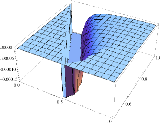
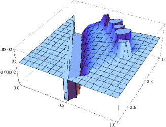
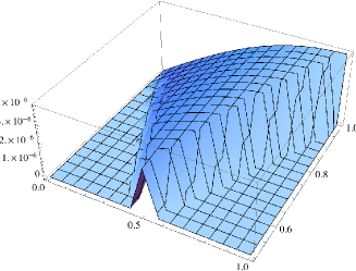
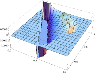
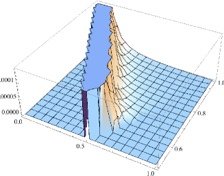
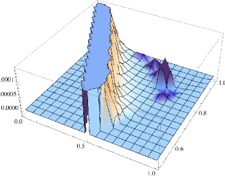
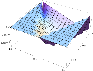
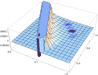
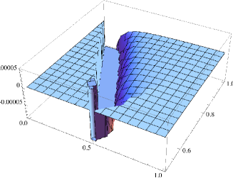
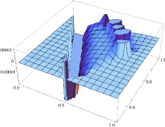
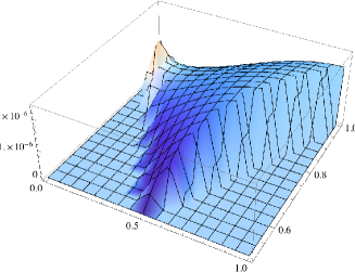
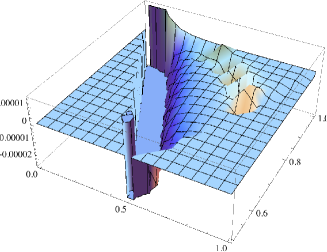
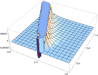
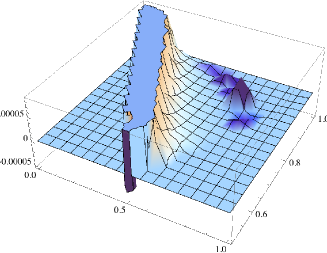
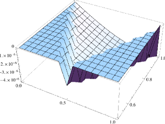
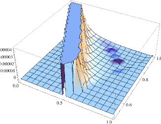
With the coefficients $\tilde{A}$ and $\tilde{B}$ given in Appendix C, the bispectrum is plotted in Figures 2 - 5 for various choices of the parameters. Figures 2 and 4 are for the choice of parameters (Appendix C: Determination of the integration constants), whereas Figures 3 and 5 are for the choice of parameters (Appendix C: Determination of the integration constants). Within each figure, four sub-cases are plotted.

From these figures, we can see that when $\delta_{\scriptscriptstyle{A}}$ and $\delta_{\scriptscriptstyle{B}}$ are taken to be zero, our result resembles the shape of $\alpha_{2}$ and $\alpha_{3}$ terms in Shinji-II , despite the fact that our integration (IV.2) is actually different from theirs. This is quite understandable from the following considerations: when we make $\delta_{\scriptscriptstyle{A}}=0=\delta_{\scriptscriptstyle{B}}$, only the positive (or negative, depending on the choice of sign for the initial condition) frequency modes exist in both regions. This makes the product of the six mode functions in (4.6), which in general has $2^{6}$ terms since each of them has two branches, collapses into one single term. Substituting this into Eqs. (IV.2) and (IV.2), we obtain

$$U^{\text{I}}\left(t^{\prime}\in(t_{i},t_{1});t\right) \propto \frac{1}{\left(k_{1}k_{2}k_{3}\right)^{3}}\frac{1}{k^{3}_{1}+k^{3}_{2}+k^{3}_{3}},$$

$$U^{\text{II}}\left(t^{\prime}\in(t_{1},t);t\right) \propto \frac{1}{\left(k_{1}k_{2}k_{3}\right)^{3}}\frac{1}{\left(k_{1}+k_{2}+k_{3}\right)^{3}}.$$

We see that the contribution from Region I has the same $k$-dependence as the $\alpha_{2}$ and $\alpha_{3}$ terms in (4.5) and (4.6) of Shinji-II . The contribution from Region II does not exist there, nor does it have the same $k$-dependence as in the relativistic cases.

The real difference comes in when we make either $\delta_{\scriptscriptstyle{A}}$ or $\delta_{\scriptscriptstyle{B}}$ nonzero. The impact of these on the shape of the bispectrum is the enhancement of the folded shape Contractions (or sometimes called the flattened shape Holman ), namely, that the bispectrum peaks at the limit $k_{2}+k_{3}-k_{1}\to 0$ and $k^{3}_{2}+k^{3}_{3}-k^{3}_{1}\to 0$. A non-zero $\delta_{\scriptscriptstyle{A}}$ for the positive frequency choice of the initial condition results in the appearance of “negative-frequency” modes in both $r^{\text{I}}_{k_{1}}(t)$ and $r^{\text{II}}_{k_{1}}(t)$, whereas a non-zero $\delta_{\scriptscriptstyle{B}}$ leads to a mixture only in $r^{\text{II}}_{k_{1}}(t)$. It’s this mixture that makes the assumption which is usually kept in the standard choice of the Bunch-Davis (BD) vacuum , that is, only positive frequency modes appear in the mode function, invalid. In fact, when we take $\eta_{i}$ to be infinite past like in the BD vacuum, $\delta_{\scriptscriptstyle{A}}$ will be zero automatically as can be seen from its definition in (C.20). When we take $\delta_{\scriptscriptstyle{A}}=0$ but $\delta_{\scriptscriptstyle{B}}\neq 0$, this is similar to the case studied in Holman and our result is consistent with theirs.

In addition, the choice of negative frequency $\tilde{A}_{-}$ essentially changes the sign of the bispectrum, and this is expected by comparing (Appendix C: Determination of the integration constants) with (Appendix C: Determination of the integration constants) .

We do not have an enhanced “squeezed” triangle signal as in the minimum scenario (though the overall magnitude there is very small), nor do we have a large local form, which is a typical result of multi-field models. This is because the interaction terms that could generate the local form are all suppressed by factors of either $c_{1}/M_{\text{pl}}$ or $\epsilon$ and are of sub-leading order [See discussions between (3.7) and (3.10)].

Now recall that in writing down (III), we have assumed that $V^{\prime}_{3}$ and $V^{\prime}_{5}$ are zero. However, this is not physically necessary since $V_{3}$ and $V_{5}$ appears neither in the background equations, nor in the linear perturbations thus not constraint by the slow-roll conditions, and a strongly varying shape of $V_{3}$ and $V_{5}$ (not to be too strong to invalidate the perturbative expansion) would actually give both a higher non-linearity and new features in the bispectrum, such as the sinusoidal running and resonant running, as shown in Contractions .

Though the final integration was separated into two distinct periods, we would like to point out that this is a result of the matching procedure employed due to the lack of exact solutions for (4.1) in our model. One should, in principle, evaluate the integration as a whole and study the shapes of the bispectrum. A possible solution is a development of the uniform approximation uniform with some numerical integration techniques involved.

(a) $\delta_{\scriptscriptstyle{A}}=0=\delta_{\scriptscriptstyle{B}}$

(b) $\delta_{\scriptscriptstyle{A}}=-0.1,~{}\delta_{\scriptscriptstyle{B}}=0$

(c) $\delta_{\scriptscriptstyle{A}}=-0.1,~{}\delta_{\scriptscriptstyle{B}}=0$

(d) $\delta_{\scriptscriptstyle{A}}=-0.1,~{}\delta_{\scriptscriptstyle{B}}=-0.1$

Figure 2: Shape of the bispectrum (truncated). $V_{3}$-term dominates, with the choice of the positive frequency.

(a) $\delta_{\scriptscriptstyle{A}}=0=\delta_{\scriptscriptstyle{B}}$

(b) $\delta_{\scriptscriptstyle{A}}=-0.1,~{}\delta_{\scriptscriptstyle{B}}=0$

(c) $\delta_{\scriptscriptstyle{A}}=0,~{}\delta_{\scriptscriptstyle{B}}=-0.1$

(d) $\delta_{\scriptscriptstyle{A}}=-0.1,~{}\delta_{\scriptscriptstyle{B}}=-0.1$

Figure 3: Shape of the bispectrum (truncated). $V_{3}$-term dominates, with the choice of the negative frequency.

(a) $\delta_{\scriptscriptstyle{A}}=0=\delta_{\scriptscriptstyle{B}}$

(b) $\delta_{\scriptscriptstyle{A}}=-0.1,~{}\delta_{\scriptscriptstyle{B}}=0$

(c) $\delta_{\scriptscriptstyle{A}}=0,~{}\delta_{\scriptscriptstyle{B}}=-0.1$

(d) $\delta_{\scriptscriptstyle{A}}=-0.1,~{}\delta_{\scriptscriptstyle{B}}=-0.1$

Figure 4: Shape of the bispectrum (truncated). $V_{5}$-term dominates, with the choice of the positive frequency.

(a) $\delta_{\scriptscriptstyle{A}}=0=\delta_{\scriptscriptstyle{B}}$

(b) $\delta_{\scriptscriptstyle{A}}=-0.1,~{}\delta_{\scriptscriptstyle{B}}=0$

(c) $\delta_{\scriptscriptstyle{A}}=0,~{}\delta_{\scriptscriptstyle{B}}=-0.1$

(d) $\delta_{\scriptscriptstyle{A}}=-0.1,~{}\delta_{\scriptscriptstyle{B}}=-0.1$

Figure 5: Shape of the bispectrum (truncated). $V_{5}$-term dominates, with the choice of the negative frequency.

IV.4 Projection onto factorizable templates

To study the quantitative behavior of the shapes of the bispectrum, in general, factorable ansatz or template functions are utilized. Among them, three are of the most importance to us Contractions ,

$$T_{\text{Orth.}}\left(k_{1},x,y\right) \equiv -18\left(\frac{1}{x^{3}}+\frac{1}{y^{3}}+\frac{1}{x^{3}y^{3}}\right)-\frac{48}{x^{2}y^{2}}$$

$$+18\left(\frac{1}{x^{2}y^{3}}+\text{5 perms.}\right),$$

$$T_{\text{Fold.}}\left(k_{1},x,y\right) \equiv 6\left(\frac{1}{x^{3}}+\frac{1}{y^{3}}+\frac{1}{x^{3}y^{3}}\right)+\frac{18}{x^{2}y^{2}}$$

$$-6\left(\frac{1}{x^{2}y^{3}}+\text{5 perms.}\right),$$

$$T_{\text{Equi.}}\left(k_{1},x,y\right) \equiv -6\left(\frac{1}{x^{3}}+\frac{1}{y^{3}}+\frac{1}{x^{3}y^{3}}\right)-\frac{12}{x^{2}y^{2}}$$ (4.17)

$$+6\left(\frac{1}{x^{2}y^{3}}+\text{5 perms.}\right),$$

where $x\equiv k_{2}/k_{1},y\equiv k_{3}/k_{1}$. Then the bispectrum (IV.2) can be cast in the form,

$$\left\langle{\cal{R}}_{\mathbf{k}_{1}}{\cal{R}}_{\mathbf{k}_{2}}{\cal{R}}_{\mathbf{k}_{3}}\right\rangle\equiv\left(2\pi\right)^{3}\delta^{3}\left(\mathbf{k}_{1}+\mathbf{k}_{2}+\mathbf{k}_{3}\right)\left(\frac{M_{*}}{h\sqrt{\beta_{0}}}\right)^{6}$$

$$~{}~{}~{}~{}~{}~{}~{}~{}~{}~{}~{}~{}~{}~{}~{}~{}~{}~{}~{}~{}~{}~{}\times T_{\text{HMT}}\left(k_{1},k_{2},k_{3}\right),$$ (4.18)

where

$$T_{\text{HMT}}=c_{\text{O}}T_{\text{Orth.}}+c_{\text{E}}T_{\text{Fold.}}+c_{\text{F}}T_{\text{Equi.}},$$ (4.19)

with

$$c_{\text{O}} = \frac{T_{\text{HMT}}\cdot T_{\text{Orth.}}}{T_{\text{Orth.}}\cdot T_{\text{Orth.}}},~{}~{}c_{\text{F}}=\frac{T_{\text{HMT}}\cdot T_{\text{Fold.}}}{T_{\text{Fold.}}\cdot T_{\text{Fold.}}},$$

$$c_{\text{E}} = \frac{T_{\text{HMT}}\cdot T_{\text{Equi.}}}{T_{\text{Equi.}}\cdot T_{\text{Equi.}}},$$ (4.20)

where the inner product is defined as Shinji-II

$$T_{1}\cdot T_{2} \equiv \sum_{\mathbf{k}_{i}}\frac{T_{1}\left(k_{1},k_{2},k_{3}\right)T_{2}\left(k_{1},k_{2},k_{3}\right)}{P_{k_{1}}P_{k_{2}}P_{k_{3}}}$$

$$\propto \int^{1}_{0}x^{4}dx\int^{1}_{1-x}y^{4}dyT_{1}(1,x,y)T_{2}(1,x,y).$$

When $\delta_{\scriptscriptstyle{A}}=0=\delta_{\scriptscriptstyle{B}}$, the projection gives the following result

$$c_{\text{O}} = M^{2}\left(1+\frac{H^{2}}{M_{*}^{2}}\right)\left(0.0033V_{3}-0.0018V_{5}\right)h^{3},$$

$$c_{\text{F}} = M^{2}\left(1+\frac{H^{2}}{M_{*}^{2}}\right)\left(0.0092V_{3}-0.0004V_{5}\right)h^{3},$$

$$c_{\text{E}} = M^{2}\left(1+\frac{H^{2}}{M_{*}^{2}}\right)\left(0.0063V_{3}-0.0036V_{5}\right)h^{3},$$

for the positive frequency, and

$$c_{\text{O}} = M^{2}\left(1+\frac{H^{2}}{M_{*}^{2}}\right)\left(-0.0004V_{3}+0.0002V_{5}\right)h^{3},$$

$$c_{\text{F}} = M^{2}\left(1+\frac{H^{2}}{M_{*}^{2}}\right)\left(-0.0001V_{3}+0.0000V_{5}\right)h^{3},$$

$$c_{\text{E}} = M^{2}\left(1+\frac{H^{2}}{M_{*}^{2}}\right)\left(-0.0008V_{3}+0.0005V_{5}\right)h^{3}.$$

for the negative frequency. We see that the projection onto the equilateral template has the biggest magnitude for most of the cases. This is consistent with the observations in EFT that derivative coupling favors the correlation between modes with similar momenta.

However, these analyses are only very rough approximations. This is because these three bases do not form a complete basis set, as pointed out in Shinji-II , nor are they un-correlated, since we can compute correlations between them and get

$$Corr\left(\text{Equi.},\text{Orth.}\right)\sim 0.204,$$

$$Corr\left(\text{Fold.},\text{Orth.}\right)\sim-0.748,$$

$$Corr\left(\text{Fold.},\text{Equi.}\right)\sim 0.489,$$ (4.24)

which indicate that there are strong correlations between the three, where

$$Corr\left(\text{S1},\text{S2}\right)\equiv\frac{T_{\text{S1}}\cdot T_{\text{S2}}}{\sqrt{T_{\text{S1}}\cdot T_{\text{S1}}}\sqrt{T_{\text{S2}}\cdot T_{\text{S2}}}}.$$ (4.25)

When $\delta_{\scriptscriptstyle{A}}$ and $\delta_{\scriptscriptstyle{B}}$ are not zero, the bispectrum, if taken naively, diverges at the folded limit $k_{2}+k_{3}-k_{1}\to 0$ or $k^{3}_{2}+k^{3}_{3}-k^{3}_{1}\to 0$, and the above inner product fails to converge. To understand the divergence, let us look at the integration (IV.2) in Region I more closely. The divergence occurs since, in addition to (IV.3), we still have $(2^{6}-2)$-terms of the form,

$$\left(\delta_{\scriptscriptstyle{A}}\right)^{m}\left(\delta_{\scriptscriptstyle{B}}\right)^{n}\frac{1}{k^{3}_{x}+k^{3}_{y}-k^{3}_{z}}.$$ (4.26)

The denominator appears through the $d\eta^{\prime}$ integration in (IV.2). When the denominator approaches zero in the folded limit, if $\delta_{\scriptscriptstyle{A}}$ and $\delta_{\scriptscriptstyle{B}}$ are not exactly zero, these terms blow up. The divergences must be regulated away if we want to have a quantitative estimate of the projection. A possible solution is to introduce a cut-off so that the integration yields,

$$\left(\delta_{\scriptscriptstyle{A}}\right)^{m}\left(\delta_{\scriptscriptstyle{B}}\right)^{n}\frac{1}{k^{3}_{2}+k^{3}_{3}-k^{3}_{1}+k^{3}_{c}}$$ (4.27)

where

$$k_{c}=k_{c}\left(\delta_{\scriptscriptstyle{A}},\delta_{\scriptscriptstyle{B}}\right),$$ (4.28)

in order to keep (4.27) finite. As noted in Contractions , this regularization is highly model-dependent and requires some systematic study. Putting this divergence aside, we would expect that the projection onto the folded base would be enhanced significantly, in comparing with (IV.4) and (IV.4).

V Conclusions and Remarks

We have studied in this paper non-Gaussianity of the primordial perturbations in a single scalar field with the slow-roll conditions in the framework of the Hořava-Lifshitz gravity with the projectability condition and an arbitrary coupling constant $\lambda$, refferred to as the HMT model.

With some reasonable assumptions, we have found that the leading order terms in self-interaction of the HMT model are of order $\epsilon^{3/2}\hat{\alpha}_{n}$, where $\hat{\alpha}_{n}$ are dimensionless constants, defined as $V_{n}\equiv\hat{\alpha}_{n}/M^{4}_{\text{pl}}$, and $V_{n}$ are the coupling coefficients of sixth order derivative operators of the scalar field, and have no contributions to the power spectra and indices, as shown explicitly in Inflation . Clearly, by properly choosing those coefficients, a large non-Gaussianity is possible. This is different from the standard result of minimum scenario in general relativity, where the interaction terms are of order $\epsilon^{2}$ Madalcena ; Weinberg05 .

We have also investigated how the modified dispersion relation affects the evolution of the mode function and in turn the bispectrum, using the matching method proposed in TransPl . By dividing the history of inflation into three regions, in which the dispersion relation takes different asymptotic forms, the gauge-invariant scalar perturbation ${\cal{R}}$ has different asymptotic solutions. In particular, we have found that the mode function is in general a superposition of oscillatory functions. This is different from the standard choice of the Bunch-Davis vacuum, where only one positive frequency branch of the plane wave is selected, and results in an enhancement of the folded shape in the bispectrum.

Due to the existence of a UV region, the bispectrum is enhanced, and gives rise to a large nonlinearity parameter $f_{\text{NL}}$ [cf. Eq.(4.13)], as long as $M_{*}$, above which the non-linear terms in the dispersion relation dominate, isn’t much lower than the Planck scale [See (4.14) and (4.15)].

We would also like to summarize the assumptions made along the analysis, as the invalidation of any of these assumptions will certainly change some of the conclusions. In particular, in obtaining the leading order term in the self-interaction, we made the assumption that $c_{1}\sim M_{*}\ll M_{\text{pl}}$. This eliminates a great number of terms which are not of order $\delta\chi^{3}$ in the third order expansion, and makes all terms that will give non-local effect (or local shape bispectrum) of sub-leading order. However, the phenomenological upper bound on $M_{*}$ for the projectable version of the HL theory is not established yet LMW . Dropping this assumption will bring back a lot of terms and enhance the local shape signal in the bispectrum.

We’ve also kept the assumption made in Inflation that $V^{\prime}_{n}\simeq 0$. For $V_{1},V_{2}$ and $V_{4}$, this assumption further eliminate some possible contributions to the leading order effect. For $V_{3}$ and $V_{5}$, as noted in the discussion at the end of Part.C in Section IV, if this assumption is dropped, new features (sharp and periodic shapes) will appear. The condition $H/M_{*}<<1$ has been also assumed to obtain an expression of the power spectrum similar to that of GR. However, if this is dropped out, the power spectrum will receive large corrections, as noted in Inflation .

By dividing the time of interest into three regions, we have assumed that the period of dominance of the $k^{4}$ term in the dispersion relation is so short that its effect can be incorporated into the small parameter $\delta_{\scriptscriptstyle{B}}$. This is a strong assumption, as noted in NaD ; PPGW . During this period of time, $\omega^{2}_{k}$ may actually go below $H^{2}$ and then the mode function will be no longer oscillating, but grow with the scale factor $a$. This is an important problem and deserves further investigations.

Acknowlodgements

We would also like to express our gratitude to V. H. Satheeshkumar, who checked carefully some of our calculations, and to Shinji Mukohyama for valuable discussions and suggestions. AW and YH would like to thank Zhejiang University of Technology for the hospitality where most of the work was done. AW is supported in part by the DOE Grant, DE-FG02-10ER41692.

Appendix A: Scalar perturbations in HMT Model

For the reader’s convenience, we present here the linearized perturbations and the corresponding constraints and field equations that were first obtained in Inflation . These will be used in obtaining the cubic action of self-interaction. Below we shall choose the Newtonian quasi-longitudinal gauge (3.3) . The variable $\psi$ defined as part of the perturbations to the 3-metric $g_{ij}$ in that paper is related to $\zeta$ used here via the relation,

$$\psi\simeq-\zeta.$$ (A.1)

The constraint equations to first order are then given by,

$$\int d^{3}x\Bigg{\{}\partial^{2}\psi-\frac{1}{2}\big{(}3\lambda-1\big{)}{\cal H}\Big{[}3\psi^{\prime}+\partial^{2}B\Big{]}\Bigg{\}}$$

$$=4\pi G\int d^{3}x\Bigg{\{}f\bar{\chi}^{\prime}\delta{\chi}^{\prime}+\Big{(}a^{2}{V}^{\prime}+\frac{V_{4}}{a^{2}}\partial^{4}\Big{)}\delta\chi\Bigg{\}},~{}~{}~{}~{}~{}$$ (A.2)

$$(3\lambda-1){\psi}^{\prime}-(1-\lambda)\partial^{2}B=8\pi Gf\bar{\chi}^{\prime}\delta\chi,$$ (A.3)

$$2{\cal{H}}\psi+\big{(}1-\lambda\big{)}\big{(}3\psi^{\prime}+\partial^{2}B\big{)}$$

$$~{}~{}~{}~{}~{}=8\pi G\Big{[}\big{(}{c}^{\prime}_{1}\bar{\chi}^{\prime}+{c}_{1}{\cal H}-f\bar{\chi}^{\prime}\big{)}\delta\chi+{c}_{1}\delta\chi^{\prime}\Big{]},$$ (A.4)

$$\psi=4\pi G{c}_{1}\delta\chi.$$ (A.5)

The trace- and traceless-dynamical equations are, respectively, given by

$$\psi^{\prime\prime}+2{\cal{H}}\psi^{\prime}+\frac{1}{3}\partial^{2}\big{(}B^{\prime}+2{\cal{H}}B\big{)}$$

$$~{}~{}~{}~{}-\frac{2}{3(3\lambda-1)}\Bigg{(}1+\frac{\alpha_{1}}{a^{2}}\partial^{2}+\frac{\alpha_{2}}{a^{4}}\partial^{4}\Bigg{)}\partial^{2}\psi$$

$$~{}~{}~{}~{}+\frac{2}{3(3\lambda-1)a}\partial^{2}\big{(}\hat{A}\psi-\hat{\delta{A}}\big{)}$$

$$~{}~{}~{}~{}=\frac{8\pi G}{3\lambda-1}\Big{(}f\bar{\chi}^{\prime}\delta\chi^{\prime}-a^{2}{V}^{\prime}\delta\chi\Big{)},$$ (A.6)

$$\psi-\big{(}B^{\prime}+2{\cal{H}}B\big{)}+\frac{1}{a^{2}}\Big{(}\alpha_{1}+\frac{\alpha_{2}}{a^{2}}\partial^{2}\Big{)}\partial^{2}\psi$$

$$~{}~{}~{}-\frac{1}{a}\Big{(}\hat{A}\psi-\hat{\delta{A}}\Big{)}=0,$$ (A.7)

where

$$\alpha_{1} \equiv \frac{8g_{2}+3g_{3}}{M^{2}_{\text{pl}}/2},\;\;\;\alpha_{2}\equiv\frac{8g_{7}-3g_{8}}{M^{4}_{\text{pl}}/4}.$$ (A.8)

The modified Klein-Gordon equation reads

$$f\Big{\{}\delta\chi^{\prime\prime}+2{\cal H}\delta\chi^{\prime}-\bar{\chi}^{\prime}\left[3\psi^{\prime}+\partial^{2}B\right]\Big{\}}+a^{2}V^{\prime\prime}\delta\chi$$

$$~{}~{}~{}~{}=2\Bigg{(}\frac{1}{2}+{V}_{1}-\frac{{V}_{2}+{V}^{\prime}_{4}}{a^{2}}\partial^{2}-\frac{{V}_{6}}{a^{4}}\partial^{4}\Bigg{)}\partial^{2}\delta\chi$$

$$~{}~{}~{}~{}~{}~{}~{}~{}~{}~{}+\frac{1}{a}\partial^{2}\Big{[}2\hat{A}\left({c}^{\prime}_{1}-{c}_{2}\right)\delta\chi+c_{1}\hat{\delta{A}}\Big{]}.$$ (A.9)

Solving the above constraints and field equations yields $B$ and other variables in terms of $\zeta$,

$$B = \frac{1}{|c^{2}_{\psi}|}\left(\partial^{-2}\zeta^{\prime}\right)-\frac{2f\bar{\chi}^{\prime}}{(1-\lambda)c_{1}}\left(\partial^{-2}\zeta\right),$$ (A.10)

$$\frac{\delta\hat{A}}{a} = \left[1+\frac{\alpha_{1}}{z^{2}}\partial^{2}+\frac{\alpha_{2}}{a^{4}}\partial^{4}-\bar{A}\right]\zeta+\frac{1}{|c^{2}_{\psi}|}\left(\partial^{-2}\zeta^{\prime\prime}\right)$$ (A.11)

$$+\left[\frac{2f\bar{\chi}^{\prime 2}}{(1-\lambda)c_{1}}\frac{c^{\prime}_{1}}{c_{1}}+\frac{2V^{\prime}}{a^{2}(1-\lambda)c_{1}}\right]\left(\partial^{-2}\zeta\right)$$

$$-\left[\frac{2f\bar{\chi}^{\prime}}{(1-\lambda)c_{1}}-\frac{2{\cal{H}}}{|c^{2}_{\psi}|}\right]\left(\partial^{-2}\zeta^{\prime}\right),$$

$$\delta\chi = -\left(4\pi Gc_{1}\right)^{-1}\zeta,$$ (A.12)

where $c^{2}_{\psi}\equiv(\lambda-1)/(1-3\lambda)$, and $\left(\partial^{-2}\partial^{2}\right)\zeta=\zeta$.

The quantity

$${\cal{R}} \equiv \psi+\frac{H}{\dot{\bar{\chi}}}\delta\chi,$$ (A.13)

$$= -\Big{(}1+\frac{H}{4\pi Gc_{1}\dot{\bar{\chi}}}\Big{)}\zeta,$$ (A.14)

often referred to as the comoving curvature perturbation, is also gauge-invariant. It can be shown that in terms of this quantity, the free action can be written as

$$S^{(2)}=\frac{1}{2}\int d\eta d^{3}xa^{2}h^{2}\Big{[}\beta_{0}{\cal{R}}^{\prime 2}-\beta_{4}{\cal{R}}^{2}-\beta_{1}(\partial_{i}{\cal{R}})^{2}$$

$$~{}~{}~{}~{}~{}~{}~{}~{}~{}~{}~{}~{}~{}~{}~{}~{}~{}~{}~{}~{}~{}~{}~{}~{}~{}~{}~{}~{}~{}~{}~{}~{}-\beta_{2}(\partial^{2}{\cal{R}})^{2}-\beta_{3}(\partial_{i}\partial^{2}{\cal{R}})^{2}\Big{]},$$

where

$$\beta_{0} = f+4\pi Gc^{2}_{1}/|c^{2}_{\psi}|,$$

$$\beta_{1} \equiv 1+2V_{1}+2\bar{A}(c_{1}^{\prime}-c_{2})-4\pi Gc^{2}_{1}(1-\bar{A}),$$

$$\beta_{2} \equiv \frac{2}{a^{2}}\left(V_{2}+V_{4}^{\prime}+2\pi Gc^{2}_{1}\alpha_{1}\right),$$

$$\beta_{3} \equiv -\frac{2}{a^{4}}\left(V_{6}+2\pi Gc^{2}_{1}\alpha_{2}\right),$$

$$\beta_{4} \equiv \beta_{0}{\cal{Q}}-\beta_{0}\frac{h^{\prime 2}}{h^{2}}+\frac{\left(a^{2}\beta_{0}hh^{\prime}\right)^{\prime}}{a^{2}h^{2}},$$

$${\cal{Q}} \equiv \frac{1}{\beta_{0}}\Bigg{\{}a^{2}V^{\prime\prime}+\frac{4\pi Gc_{1}c^{\prime\prime}_{1}\bar{\chi}^{\prime 2}}{|c_{\psi}^{2}|}-\frac{8\pi G}{\lambda-1}f\bar{\chi}^{\prime 2}\Big{(}f-{c_{1}}^{\prime}\Big{)}$$

$$-4\pi Gc_{1}a^{2}V^{\prime}\left(3+\frac{c^{\prime}_{1}}{f|c_{\psi}^{2}|}-\frac{1}{|c_{\psi}^{2}|}\right)\Bigg{\}},$$

$$h \equiv \left(4\pi Gc_{1}+\frac{H}{\dot{\bar{\chi}}}\right)^{-1}=\frac{\delta\chi}{{\cal{R}}}.$$ (A.16)

After introducing the normalized variable

$$v\equiv z{\cal{R}},\;\;\;z^{2}\equiv a^{2}h^{2}\beta_{0},$$ (A.17)

the classical equation of motion for the mode function $v_{k}$ takes the form,

$$v^{\prime\prime}_{k}+\left(\omega^{2}_{k}+m^{2}_{\text{eff}}\right)v_{k}=0,$$ (A.18)

where

$$\omega^{2}_{k} = \frac{k^{2}}{\beta_{0}}\left(\beta_{1}+{\beta_{2}}k^{2}+{\beta_{3}}k^{4}\right),$$ (A.19)

$$-m^{2}_{\text{eff}} \equiv \frac{z^{\prime\prime}}{z}-\frac{\beta_{4}}{\beta_{0}}.$$ (A.20)

Appendix B: Self interaction of the inflaton

Under the Newtonian quasi-longitudinal gauge (3.3), with perturbations given by (III), we find that the action can be written in the form,

$$S|_{(3)} = S_{g}|^{\text{GR}}_{(3)}+S_{\chi}|^{\text{GR}}_{(3)}$$ (B.1)

$$+S_{g}|^{\text{HC}}_{(3)}+S_{A}|_{(3)}+S_{\chi}|^{\text{HL}}_{(3)},$$

where the “GR parts” are given by ,

$$S_{g}|^{\text{GR}}_{(3)} = \frac{1-3\lambda}{16\pi G}\int d\eta dxa^{2}\Bigg{\{}\frac{27}{2}{\cal{H}}^{2}\zeta^{3}$$ (B.2)

$$~{}~{}~{}~{}+9{\cal{H}}\zeta^{2}\left(3\zeta^{\prime}-\partial^{2}B\right)-2\zeta^{\prime}\left(\partial_{k}B\partial^{k}\zeta\right)$$

$$~{}~{}~{}~{}+3\Big{[}3\zeta\left(\zeta^{\prime}\right)^{2}-2{\cal{H}}\zeta\left(\partial_{k}B\partial^{k}\zeta\right)-2\zeta\zeta^{\prime}\partial^{2}B\Big{]}$$

$$~{}~{}~{}~{}+\frac{3}{1-3\lambda}\zeta\left(\partial_{ij}B\right)^{2}-\frac{3\lambda}{1-3\lambda}\zeta\left(\partial^{2}B\right)^{2}$$

$$~{}~{}~{}~{}-\frac{1+\lambda}{1-3\lambda}2\left(\partial^{2}B\right)\left(\partial_{k}B\partial^{k}\zeta\right)$$

$$~{}~{}~{}~{}+\frac{8}{1-3\lambda}\left(\partial_{ij}B\partial^{i}B\partial^{j}\zeta\right)\Bigg{\}}$$

$$-\frac{1}{16\pi G}\int d\eta dxa^{2}\Big{\{}9\Lambda a^{2}\zeta^{3}+\zeta^{2}\partial^{2}\zeta\Big{\}},$$

$$S_{\chi}|^{\text{GR}}_{(3)} = \int d\eta dxa^{2}\Bigg{\{}\frac{9\zeta^{3}}{2}\left[\frac{f(\lambda)}{2}\bar{\chi}^{\prime 2}-a^{2}V\right]$$ (B.3)

$$~{}~{}~{}~{}~{}~{}+\frac{9\zeta^{2}}{2}\Big{[}f(\lambda)\bar{\chi}^{\prime}\delta\chi^{\prime}-a^{2}V^{\prime}\delta\chi\Big{]}$$

$$~{}~{}~{}~{}~{}~{}+\frac{3\zeta}{2}\Big{[}f(\lambda)\left(\delta\chi^{\prime}\right)^{2}-a^{2}V^{\prime\prime}\delta\chi^{2}\Big{]}$$

$$~{}~{}~{}~{}~{}~{}-3\zeta f(\lambda)\bar{\chi}^{\prime}\left(\partial_{k}B\right)\left(\partial^{k}\delta\chi\right)$$

$$~{}~{}~{}~{}~{}~{}-f(\lambda)\delta\chi^{\prime}\left(\partial_{k}B\right)\left(\partial^{k}\delta\chi\right)$$

$$~{}~{}~{}~{}~{}~{}-a^{2}\frac{V^{\prime\prime\prime}}{6}\left(\delta\chi\right)^{3}\Bigg{\}}.$$

And the “HL gravitational part” is given by,

$$S_{g}|^{\text{HC}}_{(3)} = \frac{1}{16\pi G}\int d\eta dxa^{2}\Bigg{\{}-a^{2}\mathscr{L}_{V}|^{\text{HC}}_{(3)}$$

$$~{}~{}~{}~{}-\left(3\zeta\right)\frac{2}{a^{2}M^{2}_{\text{pl}}}\Big{[}\left(16g_{2}+5g_{3}\right)\left(\partial^{2}\zeta\right)^{2}$$

$$~{}~{}~{}~{}~{}~{}~{}~{}~{}~{}~{}~{}~{}~{}~{}+g_{3}\left(\partial_{ij}\zeta\right)^{2}\Big{]}$$

$$~{}~{}~{}~{}-\left(3\zeta\right)\Big{(}\frac{2}{a^{2}M^{2}_{\text{pl}}}\Big{)}^{2}\Big{[}16g_{7}\left(\partial^{2}\zeta\right)\left(\partial^{4}\zeta\right)$$

$$~{}~{}~{}~{}~{}~{}~{}+5g_{8}\left(\partial_{k}\partial^{2}\zeta\right)^{2}+g_{8}\left(\partial_{ijk}\zeta\right)^{2}\Big{]}\Bigg{\}},$$

where

$$a^{2}\mathscr{L}_{V}|^{\text{HC}}_{(3)} = \frac{2}{a^{2}M^{2}_{\text{pl}}}\Big{[}\left(-64g_{2}-20g_{3}\right)\zeta\left(\partial^{2}\zeta\right)^{2}$$

$$~{}~{}~{}~{}+\left(16g_{2}+6g_{3}\right)\left(\partial^{2}\zeta\right)\left(\partial_{k}\zeta\right)^{2}$$

$$~{}~{}~{}~{}-2g_{3}\left(\partial_{i}\zeta\partial_{j}\zeta\partial^{ij}\zeta\right)-4g_{3}\zeta\left(\partial_{ij}\zeta\right)^{2}\Big{]}$$

$$+\Big{(}\frac{2}{a^{2}M^{2}_{\text{pl}}}\Big{)}^{2}\Big{[}-12g_{8}\left(\partial_{ij}\zeta\partial_{k}\zeta\partial^{ijk}\zeta\right)$$

$$~{}~{}~{}~{}+16g_{8}\left(\partial_{i}\zeta\partial_{j}\partial^{2}\zeta\partial^{ij}\zeta\right)$$

$$~{}~{}~{}~{}-\left(32g_{7}+20g_{8}\right)\left(\partial^{2}\zeta\partial_{k}\zeta\partial^{k}\partial^{2}\zeta\right)$$

$$~{}~{}~{}~{}-30g_{8}\zeta\left(\partial_{k}\partial^{2}\zeta\right)^{2}-6g_{8}\zeta\left(\partial_{ijk}\zeta\right)^{2}$$

$$~{}~{}~{}~{}-\left(64g_{4}+20g_{5}+6g_{6}+32g_{7}\right)\left(\partial^{2}\zeta\right)^{3}$$

$$~{}~{}~{}~{}+\left(16g_{7}-4g_{5}-3g_{6}\right)\left(\partial^{2}\zeta\right)\left(\partial_{ij}\zeta\right)^{2}$$

$$~{}~{}~{}~{}-g_{6}\left(\partial^{ij}\zeta\partial_{jk}\zeta\partial_{i}\partial^{k}\zeta\right)$$

$$~{}~{}~{}~{}-96g_{7}\zeta\partial^{2}\zeta\partial^{4}\zeta+8g_{7}\partial^{4}\zeta\left(\partial_{k}\zeta\right)^{2}\Big{]}.$$

The “gauge part” is given by,

$$S_{A}|_{(3)} = \frac{1}{16\pi G}\int d\eta dxa^{2}\Bigg{\{}2\bar{A}\zeta^{2}\left(\partial^{2}\zeta\right)+2\bar{A}\zeta\left(\partial_{k}\zeta\right)^{2}$$ (B.6)

$$~{}~{}~{}~{}+4\zeta\left(\partial^{2}\zeta\right)\delta A+2\left(\partial_{k}\zeta\right)^{2}\delta A\Bigg{\}}.$$

Finally, the “HL matter part” is given by

$$S_{\chi}|^{\text{HL}}_{(3)} = \int d\eta dxa^{2}\Bigg{\{}\frac{9\zeta^{2}}{2}\Big{[}-\frac{V_{4}}{a^{2}}\left(\partial^{4}\delta\chi\right)+\bar{A}c_{1}\left(\partial^{2}\delta\chi\right)\Big{]}$$

$$~{}~{}~{}~{}~{}~{}+\left(3a^{2}\zeta\right)\Big{[}\mathscr{L}_{\chi}|^{\text{HL}}_{(2)}\Big{]}+a^{2}\Big{[}\mathscr{L}_{\chi}|^{\text{HL}}_{(3)}\Big{]}\Bigg{\}},$$

with

$$\mathscr{L}_{\chi}|^{\text{HL}}_{(2)} = -V_{4}\Big{[}{\cal{P}}_{2}|_{(2)}\Big{]}-\left(\frac{1}{2}+V_{1}\right)a^{-2}\left(\partial_{k}\delta\chi\right)^{2}$$ (B.8)

$$-\frac{V_{2}}{a^{4}}\left(\partial^{2}\delta\chi\right)^{2}-\frac{V^{\prime}_{4}}{a^{4}}\delta\chi\left(\partial^{4}\delta\chi\right)$$

$$-\frac{V_{6}}{a^{6}}\left(\partial^{2}\delta\chi\right)\left(\partial^{4}\delta\chi\right)+\frac{\bar{A}c^{\prime}_{1}}{a^{2}}\delta\chi\left(\partial^{2}\delta\chi\right)$$

$$+\bar{A}c_{1}\Big{[}{\cal{P}}_{1}|_{(2)}\Big{]}+\frac{\bar{A}c_{2}}{a^{2}}\left(\partial_{k}\delta\chi\right)^{2}$$

$$+\frac{c_{1}\delta A}{a^{2}}\left(\partial^{2}\delta\chi\right),$$

$$\mathscr{L}_{\chi}|^{\text{HL}}_{(3)} = 2a^{-2}\left(\frac{1}{2}+V_{1}\right)\zeta\left(\partial_{k}\delta\chi\right)^{2}-\frac{V^{\prime}_{1}}{a^{2}}\delta\chi\left(\partial_{k}\delta\chi\right)^{2}$$ (B.9)

$$-2\frac{V_{2}}{a^{2}}\left(\partial^{2}\delta\chi\right)\Big{[}{\cal{P}}_{1}|_{(2)}\Big{]}-\frac{V^{\prime}_{2}}{a^{4}}\left(\delta\chi\right)\left(\partial^{2}\delta\chi\right)^{2}$$

$$-\frac{V_{3}}{a^{6}}\left(\partial^{2}\delta\chi\right)^{3}-V_{4}\Big{[}{\cal{P}}_{2}|_{(3)}\Big{]}$$

$$-V^{\prime}_{4}\left(\delta\chi\right)\Big{[}{\cal{P}}_{2}|_{(2)}\Big{]}-\frac{V^{\prime\prime}_{4}}{2a^{4}}\left(\delta\chi\right)^{2}\left(\partial^{4}\delta\chi\right)$$

$$-\frac{V_{5}}{a^{6}}\left(\partial^{4}\delta\chi\right)\left(\partial_{k}\delta\chi\right)^{2}$$

$$-\frac{V^{\prime}_{6}}{a^{6}}\left(\delta\chi\right)\left(\partial^{2}\delta\chi\right)\left(\partial^{4}\delta\chi\right)$$

$$-\frac{V_{6}}{a^{6}}\Big{[}(\partial^{2}\delta\chi)\left(a^{4}{\cal{P}}_{2}|_{(2)}\right)+(\partial^{4}\delta\chi)\left(a^{2}{\cal{P}}_{1}|_{(2)}\right)\Big{]}$$

$$+\bar{A}c_{1}\Big{[}{\cal{P}}_{1}|_{(3)}\Big{]}+\bar{A}c^{\prime}_{1}\left(\delta\chi\right)\Big{[}{\cal{P}}_{1}|_{(2)}\Big{]}$$

$$+\frac{\bar{A}}{a^{2}}\frac{c^{\prime\prime}_{1}}{2}\left(\delta\chi\right)^{2}\left(\partial^{2}\chi\right)$$

$$+\frac{\bar{A}}{a^{2}}\Big{[}-2c_{2}\zeta+c^{\prime}_{2}\delta\chi\Big{]}\left(\partial_{k}\delta\chi\right)^{2}$$

$$+\frac{\delta A}{a^{2}}\Big{[}c^{\prime}_{1}\delta\chi\left(\partial^{2}\delta\chi\right)+c_{1}a^{2}{\cal{P}}_{1}|_{(2)}$$

$$~{}~{}~{}~{}~{}~{}~{}~{}+c_{2}\left(\partial_{k}\delta\chi\right)^{2}\Big{]},$$

where

$$a^{2}{\cal{P}}_{1}|_{(2)} = \left(\partial_{k}\zeta\right)\left(\partial^{k}\delta\chi\right)-2\zeta\left(\partial^{2}\delta\chi\right),$$

$$a^{4}{\cal{P}}_{2}|_{(2)} = \Big{[}\left(\partial_{k}\delta\chi\right)\left(\partial^{k}\partial^{2}\zeta\right)+2\left(\partial_{k}\zeta\right)\left(\partial^{k}\partial^{2}\delta\chi\right)\Big{]}$$

$$+2\left(\partial_{ij}\zeta\right)\left(\partial^{ij}\delta\chi\right)-4\zeta\left(\partial^{4}\delta\chi\right),$$

$$a^{2}{\cal{P}}_{1}|_{(3)} = 3\zeta^{2}\partial^{2}\delta\chi,$$

$$a^{4}{\cal{P}}_{2}|_{(3)} = 8\zeta^{2}\partial^{4}\delta\chi-8\zeta\left(\partial_{ij}\zeta\right)\left(\partial^{ij}\delta\chi\right)$$

$$-4\zeta\Big{[}\left(\partial_{k}\delta\chi\right)\left(\partial^{k}\partial^{2}\zeta\right)+2\left(\partial_{k}\zeta\right)\left(\partial^{k}\partial^{2}\delta\chi\right)\Big{]}$$

$$+\left(\partial^{i}\zeta\right)\Big{[}\left(\partial^{j}\zeta\right)\left(\partial_{ij}\delta\chi\right)+\left(\partial^{j}\delta\chi\right)\left(\partial_{ij}\zeta\right)\Big{]}.$$

One can further substitute $\delta\chi,B$ and $\delta A$ in terms of $\zeta$ into Eqs. (A.10)-(A.12). See Collins for a very good and detailed review of the subject.

Appendix C: Determination of the integration constants

We find that in the original work TransPl , one of $B_{1}$ and $B_{2}$ must be zero in the case of the Corley-Jacobson dispersion with $b_{m}>0$. In fact, considering their equations (134) and (135), we find that the terms in the parentheses

$$B_{1} \propto \left(\text{cos}~{}y_{1}-i~{}\text{sin}~{}y_{1}-e^{\mp i\pi\nu}\text{cos}~{}x_{1}+ie^{\mp i\pi\nu}\text{sin}~{}x_{1}\right)$$

$$= e^{-iy_{1}}-e^{\mp i\pi\nu}e^{-ix_{1}}=e^{-iy_{1}}\left(1-e^{\mp i\pi\nu}e^{-i\pi\nu}\right),$$

$$B_{2} \propto \left(\text{cos}~{}y_{1}+i~{}\text{sin}~{}y_{1}-e^{\mp i\pi\nu}\text{cos}~{}x_{1}-ie^{\mp i\pi\nu}\text{sin}~{}x_{1}\right)$$ (C.1)

$$= e^{iy_{1}}-e^{\mp i\pi\nu}e^{ix_{1}}=e^{iy_{1}}\left(1-e^{\mp i\pi\nu}e^{+i\pi\nu}\right),$$

where we have used the definition of $x$ and $y$ in equation (128), $x=y+\pi\nu$. One immediately sees that either $B_{1}\neq 0,B_{2}=0$ (upper signs, no excitation and only “positive frequencies” exist), or $B_{1}=0,B_{2}\neq 0$ (lower signs, complete excitation and only “negative frequencies” exist). Similar problems occur for their $A_{1}$ and $A_{2}$ too (take the large argument asymptotes of the Bessell functions). We believe this is an artifact of the approximation procedure, and that in general, both the “positive-” and “negative-frequency” modes should appear and the magnitude of the “negative-frequency” modes should be limited by considerations from the back-reaction problem back ; Holman .

Below we re-derive the coefficients following the BM guidelines of matching, but within our concrete model. From (Appendix A: Scalar perturbations in HMT Model), the mode function $r_{k}(t)$ satisfies the EoM

$$\ddot{r}_{k}(t)+\left(3H+m^{2}+\frac{\omega^{2}_{k}}{a^{2}}\right)r_{k}(t)=0,$$ (C.2)

where $m^{2}=\beta_{4}/\beta_{0}$, $\omega^{2}_{k}$ is the same as defined in Eq. (A.19) and a dot represents differential w.r.t time $t$. In Region I where the nonlinear effects in the dispersion dominates, the solution takes the asymptotic form (below we use $t$ and conformal time $\eta$ interchangeably, noting that $ad\eta=dt.$),

$$r^{\text{I}}_{k}(t) \simeq A_{1}\exp\left[-i\frac{H^{2}k^{3}}{3M^{2}}\Big{(}\eta^{3}-\eta^{3}_{i}\Big{)}\right]$$

$$+A_{2}\exp\left[+i\frac{H^{2}k^{3}}{3M^{2}}\Big{(}\eta^{3}-\eta^{3}_{i}\Big{)}\right]$$

$$= \tilde{A}_{1}\exp\left[-i\frac{H^{2}k^{3}}{3M^{2}}\eta^{3}\right]+\tilde{A}_{2}\exp\left[+i\frac{H^{2}k^{3}}{3M^{2}}\eta^{3}\right],$$

$$\tilde{A}_{1} \equiv A_{1}\exp\left[+i\frac{H^{2}k^{3}}{3M^{2}}\eta^{3}_{i}\right],$$

$$\tilde{A}_{2} \equiv A_{2}\exp\left[-i\frac{H^{2}k^{3}}{3M^{2}}\eta^{3}_{i}\right],$$ (C.3)

$$M^{-4} \equiv \frac{\beta_{3}a^{4}}{\beta_{0}}=\frac{2\left|V_{6}+2\pi Gc^{2}_{1}\alpha_{2}\right|}{f+4\pi Gc^{2}_{1}/|c^{2}_{\psi}|}.$$ (C.4)

It can be shown that $M$ here is related to $M_{*}$ defined in Inflation through $M^{4}_{*}=b_{3}M^{4}$. Since $b_{3}\sim{\cal{O}}(1)$, the condition $H^{2}/M^{2}_{*}\ll 1$ implies $H^{2}/M^{2}\ll 1$.

In Region II, the mode function is a superposition of plane waves,

$$r^{\text{II}}_{k}(t) \simeq B_{1}\exp\left[-ic_{s}k\left(\eta-\eta_{1}\right)\right]+B_{2}\exp\left[ic_{s}k\left(\eta-\eta_{1}\right)\right]$$

$$= \tilde{B}_{1}\exp\left[-ic_{s}k\eta\right]+\tilde{B}_{2}\exp\left[+ic_{s}k\eta\right],$$

$$\tilde{B}_{1} \equiv B_{1}\exp\left[+ic_{s}k\eta_{1}\right],$$

$$\tilde{B}_{2} \equiv B_{2}\exp\left[-ic_{s}k\eta_{1}\right],$$ (C.5)

$$c^{2}_{s} \equiv \frac{\beta_{1}}{\beta_{0}}=\frac{1+2V_{1}+2\bar{A}(c_{1}^{\prime}-c_{2})-4\pi Gc^{2}_{1}(1-\bar{A})}{f+4\pi Gc^{2}_{1}/|c^{2}_{\psi}|}.$$

The initial conditions are chosen such that

$$r_{k}(t_{i})=\frac{v_{k}(\eta_{i})}{z(\eta_{i})}=\frac{1}{z(\eta_{i})\sqrt{2\omega(\eta_{i})}},$$ (C.7)

whereas its initial time-derivative takes value such that the energy density is minimized at the initial time (not necessarily infinite past $\eta_{i}\to-\infty$)

$$r^{\prime}_{k}(t_{i})=\Big{(}\frac{v_{k}(\eta_{i})}{z(\eta_{i})}\Big{)}^{\prime}$$ (C.8)

$$= \pm i\frac{1}{z(\eta_{i})}\sqrt{\frac{\omega(\eta_{i})}{2}}.$$

At the time of matching between region I and II, $t_{1}$,

$$r^{\text{I}}_{k}(t_{1})=r^{\text{II}}_{k}(t_{1}),~{}~{}~{}~{}~{}r^{\prime\text{I}}_{k}(t_{1})=r^{\prime\text{II}}_{k}(t_{1}).$$ (C.9)

These four conditions (C.7)$\sim$(C.9) fix the four undetermined constants

$$\tilde{A}_{1+} = \frac{\exp\left[+i\frac{H^{2}k^{3}}{3M_{*}^{2}}\eta^{3}_{i}\right]}{z\left(\eta_{i}\right)\sqrt{2\omega\left(\eta_{i}\right)}}\Big{(}1+\frac{2i}{\eta_{i}\omega\left(\eta_{i}\right)}\Big{)},$$

$$\tilde{A}_{2+} = \frac{\exp\left[-i\frac{H^{2}k^{3}}{3M_{*}^{2}}\eta^{3}_{i}\right]}{z\left(\eta_{i}\right)\sqrt{2\omega\left(\eta_{i}\right)}}\Big{(}0-\frac{2i}{\eta_{i}\omega\left(\eta_{i}\right)}\Big{)},$$

$$\omega\left(\eta_{i}\right) \simeq \frac{k^{3}H^{2}\eta^{2}_{i}}{M_{*}^{2}},$$ (C.10)

for $r^{\prime}_{k}(t_{i})=+i\frac{1}{z(\eta_{i})}\sqrt{\frac{\omega(\eta_{i})}{2}}$ (positive frequency choice), or

$$\tilde{A}_{1-} = \frac{\exp\left[+i\frac{H^{2}k^{3}}{3M_{*}^{2}}\eta^{3}_{i}\right]}{z\left(\eta_{i}\right)\sqrt{2\omega\left(\eta_{i}\right)}}\Big{(}0+\frac{2i}{\eta_{i}\omega\left(\eta_{i}\right)}\Big{)},$$

$$\tilde{A}_{2-} = \frac{\exp\left[-i\frac{H^{2}k^{3}}{3M_{*}^{2}}\eta^{3}_{i}\right]}{z\left(\eta_{i}\right)\sqrt{2\omega\left(\eta_{i}\right)}}\Big{(}-1-\frac{2i}{\eta_{i}\omega\left(\eta_{i}\right)}\Big{)}.$$ (C.11)

for $r^{\prime}_{k}(t_{i})=-i\frac{1}{z(\eta_{i})}\sqrt{\frac{\omega(\eta_{i})}{2}}$ (negative frequency choice). And

$$\tilde{B}_{1} = \frac{e^{+ic_{s}k\eta_{1}}}{2}\Bigg{[}\left(1+\frac{k^{2}H^{2}\eta^{2}_{1}}{c_{s}M_{*}^{2}}\right)\tilde{A}_{1}\exp\left(-i\frac{H^{2}k^{3}}{3M_{*}^{2}}\eta^{3}_{1}\right)$$

$$~{}~{}~{}+\left(1-\frac{k^{2}H^{2}\eta^{2}_{1}}{c_{s}M_{*}^{2}}\right)\tilde{A}_{2}\exp\left(+i\frac{H^{2}k^{3}}{3M_{*}^{2}}\eta^{3}_{1}\right)\Bigg{]},$$

$$\tilde{B}_{2} = \frac{e^{-ic_{s}k\eta_{1}}}{2}\Bigg{[}\left(1-\frac{k^{2}H^{2}\eta^{2}_{1}}{c_{s}M_{*}^{2}}\right)\tilde{A}_{1}\exp\left(-i\frac{H^{2}k^{3}}{3M_{*}^{2}}\eta^{3}_{1}\right)$$

$$~{}~{}~{}+\left(1+\frac{k^{2}H^{2}\eta^{2}_{1}}{c_{s}M_{*}^{2}}\right)\tilde{A}_{2}\exp\left(+i\frac{H^{2}k^{3}}{3M_{*}^{2}}\eta^{3}_{1}\right)\Bigg{]}.$$

The time of matching $\eta_{1}$ (or equivalently, $t_{1}$) is a critical quantity, here we choose it to be Match

$$\omega^{2}_{k}(\eta_{1})-c^{2}_{s}k^{2}=c^{2}_{s}k^{2},$$ (C.13)

or from (A.19)

$$\beta_{3}\left(\eta_{1}\right)k^{4}+\beta_{2}\left(\eta_{1}\right)k^{2}=\beta_{1}.$$ (C.14)

Now recall that by dividing the evolution history into three regions, we implicitly assumed that the $\beta_{2}$ term was never dominant during the history of inflation, as a result, the above condition can be approximated with

$$\beta_{3}\left(\eta_{1}\right)k^{4}=\beta_{1},$$ (C.15)

which leads to

$$2\left|V_{6}+2\pi Gc^{2}_{1}\alpha_{2}\right|k^{4}H^{4}\eta^{4}_{1}=\beta_{1}.$$ (C.16)

Hence

$$\left(kH\eta_{1}\right)^{2} = c_{s}M_{*}^{2}\left(1+2\delta_{\scriptscriptstyle{B}}\right),$$

$$\eta_{1} \simeq -\frac{\sqrt{c_{s}}}{k}\frac{M_{*}}{H}\left(1+\delta_{\scriptscriptstyle{B}}\right),$$ (C.17)

where we have used the definition of $c_{s}$ and $M_{*}$, and introduced a quantity $\delta_{\scriptscriptstyle{B}}$ to denote any deviations from (C.15), for example, when we consider the $k^{4}$ term’s minimal effect on $\eta_{1}$. (In Match , it was found that a difference in this matching time could result in an unnecessary oscillatory component for the power spectrum, and we shall see below that this indeed happens through an extra oscillatory phase for the coefficients $B$.)

Looking at the equation (Appendix C: Determination of the integration constants), this choice of $\eta_{1}$ indicates that the influence of $\tilde{A}_{2}$ ($\tilde{A}_{1}$) on $\tilde{B}_{1}$ ($\tilde{B}_{2}$) is minimal. Also note that $\eta_{i}\omega\left(\eta_{i}\right)\sim({H^{2}}/{M_{*}^{2}})k^{3}\eta^{3}_{i}$ is in general a very large quantity, this allows us to make further approximations on the expressions of the coefficients $\tilde{A}$ and $\tilde{B}$ and arrive at

$$\tilde{A}_{1+} = \frac{M_{*}}{h\sqrt{\beta_{0}}\sqrt{2k^{3}}}~{}e^{+i\phi_{\scriptscriptstyle{A}}}\left(1+i\delta_{\scriptscriptstyle{A}}\right),$$

$$\tilde{A}_{2+} = \frac{-M_{*}}{h\sqrt{\beta_{0}}\sqrt{2k^{3}}}~{}e^{-i\phi_{\scriptscriptstyle{A}}}\left(i\delta_{\scriptscriptstyle{A}}\right),$$

$$\tilde{B}_{1+} = \frac{M_{*}}{h\sqrt{\beta_{0}}\sqrt{2k^{3}}}~{}e^{i\phi_{\scriptscriptstyle{B1}}}\left(1+i\delta_{\scriptscriptstyle{A}}+\delta_{\scriptscriptstyle{B}}\right),$$

$$\tilde{B}_{2+} = \frac{-M_{*}}{h\sqrt{\beta_{0}}\sqrt{2k^{3}}}\left(i\delta{\scriptscriptstyle{A}}e^{-i\phi_{\scriptscriptstyle{B1}}}+\delta_{\scriptscriptstyle{B}}e^{i\phi_{\scriptscriptstyle{B2}}}\right),$$

or

$$\tilde{A}_{1-} = \frac{M_{*}}{h\sqrt{\beta_{0}}\sqrt{2k^{3}}}~{}e^{+i\phi_{\scriptscriptstyle{A}}}\left(i\delta_{\scriptscriptstyle{A}}\right),$$

$$\tilde{A}_{2-} = \frac{-M_{*}}{h\sqrt{\beta_{0}}\sqrt{2k^{3}}}~{}e^{-i\phi_{\scriptscriptstyle{A}}}\left(1+i\delta_{\scriptscriptstyle{A}}\right),$$

$$\tilde{B}_{1-} = \frac{M_{*}}{h\sqrt{\beta_{0}}\sqrt{2k^{3}}}\left(i\delta{\scriptscriptstyle{A}}e^{i\phi_{\scriptscriptstyle{B1}}}+\delta_{\scriptscriptstyle{B}}e^{-i\phi_{\scriptscriptstyle{B2}}}\right),$$

$$\tilde{B}_{2-} = \frac{-M_{*}}{h\sqrt{\beta_{0}}\sqrt{2k^{3}}}~{}e^{-i\phi_{\scriptscriptstyle{B1}}}\left(1+i\delta_{\scriptscriptstyle{A}}+\delta_{\scriptscriptstyle{B}}\right),$$ (C.19)

where

$$\delta_{\scriptscriptstyle{A}} \equiv \frac{2}{\eta_{i}\omega\left(\eta_{i}\right)}=\frac{2M_{*}^{2}}{k^{3}\eta^{3}_{i}H^{2}},$$ (C.20)

$$\phi_{\scriptscriptstyle{A}} \equiv \frac{H^{2}k^{3}}{3M_{*}^{2}}\eta^{3}_{i},$$

$$\phi_{\scriptscriptstyle{B1}} \equiv \frac{c_{s}k\eta_{1}}{3}\left[\left(1+2\delta_{\scriptscriptstyle{B}}\right)\left(\frac{\eta_{i}}{\eta_{1}}\right)^{3}+2\left(1-\delta_{\scriptscriptstyle{B}}\right)\right],$$

$$\phi_{\scriptscriptstyle{B2}} \equiv \frac{c_{s}k\eta_{1}}{3}\left[\left(1+2\delta_{\scriptscriptstyle{B}}\right)\left(\frac{\eta_{i}}{\eta_{1}}\right)^{3}-2\left(2+\delta_{\scriptscriptstyle{B}}\right)\right].$$

References

• (1) P. Hořava, Phys. Rev. D79, 084008 (2009) [arXiv:0901.3775].
• (2) E.M. Lifshitz, Zh. Eksp. Toer. Fiz. 11, 255; 269 (1941).
• (3) D. Blas, O. Pujolas, and S. Sibiryakov, JHEP 1104, 018 (2011) [arXiv.1007.3503]; S. Mukohyama, Class. Quantum Grav. 27, 223101 (2010) [arXiv:1007.5199]; A. Padilla, J. Phys. Conf. Ser. 259, 012033 (2010) [arXiv:1009.4074]; T.P. Sotiriou, J. Phys. Conf. Ser. 283, 012034 (2011) [arXiv:1010.3218]; P. Hořava, Class. Quantum Grav. 28, 114012 (2011) [arXiv:1101.1081]; T. Clifton, P.G. Ferreira, A. Padilla, and C. Skordis, Phys. Rep. 513, 1 (2012) [arXiv:1106.2476].
• (4) T. Sotiriou, M. Visser, and S. Weinfurtner, Phys. Rev. Lett. 102, 251601 (2009) [arXiv:0904.4464]; J. High Energy Phys., 10, 033 (2009) [arXiv:0905.2798].
• (5) P. Hořava and C.M. Melby-Thompson, Phys. Rev. D82, 064027 (2010) [arXiv:1007.2410].
• (6) A. Wang and Y. Wu, Phys. Rev. D 83, 044031 (2011) [arXiv:1009. 2089].
• (7) A.M. da Silva, Class. Quan. Grav. 28, 055011 (2011) [arXiv:1009.4885].
• (8) Y.-Q. Huang and A. Wang, Phys. Rev. D83, 104012 (2011) [arXiv:1011.0739].
• (9) D.Blas, O.Pujolas, and S. Sibiryakov, Phys. Rev. Lett. 104, 181302 (2010) [arXiv:0909.3525]; JHEP 04, 018 (2011) [arXiv:1007.3503].
• (10) T. Zhu, Q. Wu, A. Wang, and F.-W. Shu, Phys. Rev. D84, 101502 (R) (2011) [arXiv:1108.1237]; T. Zhu, F.-W. Shu, Q. Wu, and A. Wang, Phys. Rev. D85, 044053 (2012) [arXiv:1110.5106].
• (11) C.W. Misner, K.S. Thorne, and J.A. Wheeler, Gravitation (W.H. Freeman and Company, San Francisco, 1973), pp.484-528.
• (12) K. Lin, A. Wang, Q. Wu, and T. Zhu, Phys. Rev. D 84, 044051 (2011) [arXiv:1106.1486].
• (13) D. Blas, O. Pujolas, and S. Sibiryakov, Phys. Lett. B 688, 350 (2010) [arXiv:0912.0550].
• (14) K. Lin, S. Mukohyama, and A. Wang, arXiv:1206.1338.
• (15) X. Gao, arXiv:0904.4187.
• (16) K. Izumi, T. Kobayashi and S. Mukohyama, JCAP, 10, 031 (2010) [arXiv:1008:1406].
• (17) D. H. Lyth and D. Wands, Phys. Lett. B524, 5 (2002) [arXiv:hep-ph/0110002]; K. Enqvist and M. S. Sloth, Nucl. Phys. B626, 395 (2002) [arXiv:hep-ph/0109214]; T. Moroi and T. Takahashi, Phys. Lett. B522, 215 (2001) [Erratum-ibid. B 539, 303 (2002)] [arXiv:hep-ph/0110096].
• (18) S. Mukohyama, JCAP, 0906, 001 (2009) [arXiv:0904.2190].
• (19) Y. Huang, A. Wang and Q. Wu, JCAP, 10, 10 (2012) [arXiv:1201.4630].
• (20) J. Schwinger, Proc. Nat. Acad. Sci. US, 46, 1401 (1961); L. V. Keldysh, Sov. Phys. JETP, 20, 1018 (1965).
• (21) J. Maldacena, JHEP 05, 013 (2003) [arXiv:astro-ph/0210603].
• (22) S. Weinberg, Phys. Rev. D72, 043514 (2005) [arXiv:hep-th/0506236].
• (23) K. Koyama, Class. Quan. Grav. 27, 124001 (2010) [arXiv:1002.0600].
• (24) X. Chen, Adv. Astron. 2010: 638979, (2010) [arXiv:1002.1416].
• (25) Planck Collaboration, arXiv:astro-ph/0604069.
• (26) D. Baumann et al., AIP Conf. Proc. 1141:10-120, 2009 [arXiv: 0811.3919].
• (27) E. Komatsu et al., Astrophys. J. Suppl. 192 18 (2011) [arXiv:1001.4538].
• (28) R. Holman and A.J. Tolley, JCAP 05, 001 (2008) [arXiv:0710.1302].
• (29) A. Wang and R. Martenns, Phys. Rev. D81, 024009 (2010) [arXiv:0907.1748]; A. Wang, D. Wands and R. Martenns, JCAP 03, 013 (2010) [arXiv:0909.5167].
• (30) J. Martin and R.H. Brandenberger, Phys. Rev. D63, 123501 (2001) [arXiv:hep-th/005209].
• (31) A. Ashoorioon, D. Chialva and U.H. Danielsson, JCAP 06, 034 (2011) [arXiv:1104.2338].
• (32) J. Martin and R.H. Brandenberger, Phys. Rev. D65, 103514 (2002) [arXiv:hep-th/0201189].
• (33) P. Creminelli, JCAP 10, 003 (2003) [arXiv:astro-ph/0306122]; N. Arkani-Hamed, P. Creminelli, S. Mukohyama and M. Zaldarriaga, JCAP 04, 001 (2004) [arXiv:hep-th/0312100]; P. Creminelli et. al., JCAP 02, 006 (2011) [arXiv:1011.3004].
• (34) S. Habib, A Heinen, K. Heitmann, G. Jungman and C. Molina-País, Phys. Rev. D70, 083507 (2004) [arXiv:astro-ph/0406134]; A. Wang, Phys. Rev. D82, 124063 (2010) [arXiv:1008.3637].
• (35) J. Martin and R.H. Brandenberger, Phys. Rev. D68, (2003) 063513 [arXiv:hep-th/0305161].
• (36) A. Wang, Q. Wu, W. Zhao and T. Zhu, arXiv:1208.5490.
• (37) H. Colins, arXiv:1101.1308.
• (38) R.H. Brandenberger and J. Martin, Phys. Rev. D71, (2005) 023504.