${{~{}~{}~{}~{}~{}~{}~{}~{}~{}~{}~{}~{}~{}~{}~{}~{}~{}~{}~{}~{}~{}~{}~{}~{}~{}~{}}^{{}^{{}^{Published~{}in~{}the~{}Astrophysical~{}Journal\,,~{}Vol.~{}764\,,~{}id.~{}27\,~{}~{}(2013)}}}}$
No pseudosynchronous rotation for terrestrial planets and moons  
 

Abstract

We reexamine the popular belief that a telluric planet or satellite on an eccentric orbit can, outside a spin-orbit resonance, be captured in a quasi-static tidal equilibrium called pseudosynchronous rotation. The existence of such configurations was deduced from oversimplified tidal models assuming either a constant tidal torque or a torque linear in the tidal frequency. A more accurate treatment requires that the torque be decomposed into the Darwin-Kaula series over the tidal modes, and that this decomposition be combined with a realistic choice of rheological properties of the mantle, which we choose to be a combination of the Andrade model at ordinary frequencies and the Maxwell model at low frequencies. This development demonstrates that there exist no stable equilibrium states for solid planets and moons, other than spin-orbit resonances.

1 Motivation

The ongoing quest for extraterrestrial life has placed exoplanets and their properties into the forefront of scientific investigation. The trend has provided additional momentum to the development of a broad variety of techniques and approaches employed in the planetary sciences. For example, the recent revival of interest in mechanics of bodily tides is partly due to the importance of the planetary spin for the prospects of finding habitable worlds near other stars.

Well-known examples of dynamical equilibria achieved via tidal coupling include our Moon, which is in a 1:1 spin-orbit resonance to the Earth, and Mercury which makes exactly three sidereal rotations over every two orbital revolutions around the Sun. Similar behaviour is expected of the growing number of known super-earths – especially if their composition happens to be similar to that of the terrestrial planets of the solar system, i.e., if they have massive solid or partially molten mantles of rocky minerals.

Unfortunately, some of the published far-reaching conclusions about specific exoplanets are based on incomplete or  ad hoc  models which should never be used for solid materials, including those with partial melt. Both these models, introduced by Goldreich (1966) mainly for the ease of analytical treatment, predict quasi-static pseudosynchronous rotation states, with the planet being trapped in a slowly changing equilibrium state at a faster-than-synchronous rotation rate and a vanishing orbit-averaged tidal torque. Except in specific (very narrow) frequency bands, these models are incompatible with the rheological properties of realistic mantles and crusts. Analysis based on actual rheologies demonstrates the impossibility of pseudosynchronous rotation for homogeneous terrestrial objects. Whether this prohibition extends to planets and moons with internal or surface oceans remains an open issue and needs further research.

2 The constant angular lag model

A consistent linear theory of bodily tides is based on Fourier decomposition of the tide, with subsequent inclusion of the response at each separate mode. The ensuing level of complexity has tempted many to circumvent it by developing simpler approaches. Serving as good illustrations and reflecting some qualitative aspects of the tidal interaction, such models are not necessarily applicable for quantitative purposes (Efroimsky & Lainey 2007) and should certainly be eschewed when fine features of near-resonant dynamics are explored.

2.1 The essence of the method

One, often-used, toy model prescribes:

(a) to set both the Love number $\,k_{2}\,$ and geometric lag $\,\epsilon_{g}\,$ frequency-independent;
 

(b) to insert their values into the popular short formula

$${\cal{T}}_{z}~{}=~{}\frac{3}{2}~{}G\,M_{1}^{\,2}~{}\frac{R^{5}}{r^{6}}~{}k_{2}\,\sin 2\epsilon_{g}$$ (1a)

          for the polar component of the torque wherewith a tide-raising perturber of mass $$\,M_{1}\, \,R\, \,r\, \,i\,$$
           acts on a tidally perturbed body of radius located at a distance , the obliquity
           assumed small; and
 

(c)  to combine formula (1a) with the assumption that the angle $\,\epsilon_{g}\,$ stays constant while
            the tide-raising perturber stays on one side of the bulge (in the sense of the directions
            as seen from the perturbed body’s centre).
 

For a nonzero eccentricity $\,e\,$, and in a sufficient proximity of the 1:1 resonance, the relative orientation of the perturber and the bulge changes twice over an orbital period. Hence, within this model, the angle $\,\epsilon_{g}\,$ is set, by hand, to change its sign abruptly twice in a cycle, while keeping its magnitude $\,|\,\epsilon_{g}\,|\,$ fixed. Therefore the model can be written down as

$${\cal{T}}_{z}~{}=~{}\frac{3}{2}~{}G\,M_{1}^{\,2}~{}\frac{R^{5}}{r^{6}}~{}k_{2}\,\sin 2|\epsilon_{g}|~{}\,\mbox{Sgn}\,(\dot{\nu}\,-\,\dot{\theta})\,~{},$$ (1b)

$\theta$ and $\dot{\theta}$ being the perturbed body’s sidereal angle and spin rate, and $\nu$ being the true anomaly.

Historically, the method dates back to the paper by MacDonald (1964) and therefore is often referred to as the MacDonald torque (e.g., Touma & Wisdom 1994, Section 2.7.1).

The approach is also called the  constant angular lag model  or the  constant tidal torque model, both names being somewhat misleading. Indeed, in the vicinity of the 1:1 resonance the sign of the lag (and the torque) is set positive or negative, when the bulge falls behind or advances relative to the direction towards the perturber. So both quantities change their sign twice over a period – a circumstance that makes the term constant inappropriate. Furthermore, the torque depends upon the distance and is always evolving in time unless the orbit is circular.

The abrupt switch of the sign of the torque (2.1), with its magnitude staying unchanged, is quite a contrived assertion  which by itself indicates that the model is unphysical. A deeper, mathematical, objection will be brought up in Section 2.4.

Saying goodbye to the constant-angular-lag model will not be easy, because it has been a textbook standard for nearly half a century. Given the attractive simplicity of the model, one will always be tempted to enquire if perhaps it would still be producing at least qualitative results of some value. To see that it would not, we shall have to scrutinise the principal outcomes of the model.

The perturber’s orbit is set to lie in the equatorial plane of the perturbed body; in other words, the obliquity is set zero. Two special situations of interest emerge here. One is the case of exact synchronism, the other being the case of a vanishing average tidal torque. Both settings were explored by Goldreich (1966) whose results are explained in detail by Murray & Dermott (1999).

2.2 The synchronous spin case

Suppose the tidally-perturbed body on an elliptic ($\,e\,\neq\,0\,$) orbit is caught into the 1:1 spin-orbit resonance: $\,n=\dot{\theta}\,$. Then, as explained in Section 5.2 of Murray & Dermott (1999), the angular motion rate $\,\dot{\theta}\,$ exceeds $\,n\,$ over exactly one half of the orbital time period, and falls short of $\,n\,$ during the other half of the period. Correspondingly, the tidal torque $\,{\cal{T}}_{z}\,$ is positive (accelerating) through the former half of the period, and is negative (decelerating) through the latter half. The instantaneous tidal torque is proportional to a negative power of the instantaneous distance $\,r\,$ between the bodies. As depicted in Figure 5.3 in Ibid, when the disturbed body’s angular motion is faster than the mean motion, the bodies are closer, so the positive (spinning up) tidal torque is larger in absolute value than the negative torque for the other half of the period. Thus the resultant orbit-averaged torque $\,\langle\,{\cal{T}}_{z}\,\rangle\,$ is positive, and the net effect is to accelerate the tidally perturbed body’s spin. (Recall that the undisturbed body is assumed to be spherical or oblate, so the tidal torque is the only one coming into play.)

2.3 The case of vanishing tidal torque

The second important application of the constant angular lag model is the situation where the orbit-average tidal torque vanishes: $\,\langle\,{\cal{T}}_{z}\,\rangle\,=0\,$. Vanishing of the average tidal torque entails a dynamical equilibrium: the tidally disturbed body keeps rotating at a steady spin rate. A calculation of this rate, borrowed from Goldreich (1966), is presented in Murray & Dermott (1999) and is often cited in the literature. According to that development, the equilibrium is achieved, for a zero obliquity, at the spin rate of

$$\stackrel{{\scriptstyle\mbox{\bf{\LARGE{$\,\cdot$}}}}}{{\theta}}_{\textstyle{{}_{\rm eq}}}\,=\,n\,\left(\,1\,+\,\frac{19}{2}~{}e^{2}\,\right)~{}\,,$$ (2)

$e\,$ being the eccentricity. At first glance, the result looks unassailable. Indeed, for $\,\dot{\theta}=n\,$, the bulge is lagging behind the central line over one half of the time period (around the periastron), so the torque accelerates the rotation. Over the other half of the period, the torque decelerates, being weaker due to a larger distance. So the state $\,\dot{\theta}=n\,$ looks unstable, as the overall average torque seems to be accelerating.

It is however well known that the Moon is not staying in this pseudosynchronous regime (which would be 3% faster than the synchronous rotation wherein the Moon is presently locked). Murray & Dermott (1999) point at the lunar quadrupole moment as the reason why the Moon is not pseudosynchronous. A deeper reason though lies in the constant geometric lag model being genuinely flawed, and in the entire calculation leading to (2) being invalid.

2.4 A major objection against the constant-angular-lag model

As well known, the generic expression for the tidal amendment to the perturbed body’s potential is furnished by a Fourier series developed by Kaula (1964). We term it the Darwin-Kaula expansion, as a partial sum of that series was written down by Darwin (1879). Accordingly, the generic expression of the tidal torque also must look as an infinite series. The series remains infinite even if we include into it only the degree-2 terms, i.e., those proportional to the quadrupole Love number $\,k_{2}\,$. The very fact that the expansion for the torque can be wrapped into a short and neat form (2.1) is an indicator of some extra, very special assumption being involved.

As was pointed out in Williams & Efroimsky (2012), such an assumption indeed is present in the constant-angular-lag model, though this assumption is never stipulated explicitly. The situation is elucidated in all detail in the paper by Efroimsky & Makarov (2013) to which we refer the reader. Here we shall provide only a brief summary.

As explained in Williams & Efroimsky (2012), the afore-presented concise expression (2.1) for the torque is equivalent to the full Darwin-Kaula expansion for the potential, only if the following assumptions are made:

• In all terms of the Darwin-Kaula series for the tidal amendment to the potential of the perturbed body, i.e, for all Fourier tidal modes $\,\omega_{lmpq}\,$, the time lags are endowed with the same, frequency-independent value $\,\Delta t\,$.

• The obliquity is set small.

• Only the terms with $\,l=m=2\,$ are retained, and the Love number $\,k_{2}\,$ entering these terms is assumed frequency-independent. Here the degree $\,l\,$ and the order $\,m\,$ are the first two integers of the four-number set $\,lmpq\,$ used to number the Fourier modes showing up in the Darwin-Kaula expansion.
  

The so-processed Darwin-Kaula series for the tidal potential becomes equivalent to a concise expression (equation 16b in Ibid.) wherefrom our expression (2.1) for the torque ensues.

Alternatively, the above three assumptions could be applied directly to the Darwin-Kaula expansion for the tidal torque. Once again, the outcome would be the above expression (2.1) for the torque. This is demonstrated in Efroimsky & Makarov (2013, equation 34).

Under the three assumptions, the instantaneous geometric lag angle turns out to be

$$\epsilon_{g}\,\equiv~{}(\dot{\nu}-\dot{\theta})\,\Delta t~{}\,,$$ (3)

$\,\Delta t\,$ being the frequency-independent time lag, $\,\nu\,$ being the true anomaly of the perturber, and $\,\theta\,$ being the sidereal angle of the tidally perturbed body. From this expression, it is straightforward that the validity of formula (2.1) is incompatible with the geometric lag being constant. Indeed, the road to (2.1) is paved with the aforementioned three assumptions, one of which being that of a constant $\,\Delta t\,$. As can be observed from (3), the latter is incompatible with the geometric lag being constant, unless the eccentricity is nil.

On all these grounds, the constant-geometric-lag (constant-torque) model should be discarded as such.

3 Pseudosynchronism in the constant time lag model

As distinct from the constant geometric lag approach, the constant time lag model sets the time delay $\,\Delta t\,$ independent of the tidal mode frequency. Pioneered by Darwin (1879), this assumption was a part of numerous works, e.g., Hut (1981), Eggleton et al. (1998). The assumption was also the base for one of the two models considered by Goldreich & Peale (1966, equation 23), the other model addressed in that paper being the afore-discarded constant geometric lag method.

The constant time lag model is unique, in that it makes the full Darwin-Kaula expansion for the tidal potential (or torque) equivalent to a much shorter and simpler expression. In regard to the tidal potential, this is the equivalence of the full series (16) and a simpler expression (15) in our preceding paper Efroimsky & Makarov (2013). In application to the torque, this is the equivalence of the appropriate full series to the simpler expression (34) in Ibid.

If we agree to limit our approximation to the lowest degree and order, $\,l=m=2\,$, the aforementioned simpler expressions read as

$$U(\mbox{{\boldmath$\vec{r}$}})=~{}-~{}\frac{3}{4}~{}G\,M_{1}\,k_{2}~{}\frac{\,R^{\textstyle{{}^{5}}}\,}{\,r^{6}\,}~{}\cos(\,2\,(\dot{\nu}-\dot{\theta})\,\Delta t\,)\,=~{}\frac{3}{4}~{}G\,M_{1}\,k_{2}~{}\frac{\,R^{\textstyle{{}^{5}}}\,}{\,r^{6}\,}~{}\cos(\,2\,|\,\dot{\nu}-\dot{\theta}\,|\,\Delta t\,)\,~{},\,~{}\,$$ (4)

for the potential, and as

$${\cal{T}}_{z}\,=\,\frac{\textstyle 3}{\textstyle 2}~{}{G\;M_{1}^{\,2}}\,k_{2}\;\frac{R^{5}}{r^{\textstyle{{}^{6}}}}\;\sin(\,2\,(\dot{\nu}-\dot{\theta})\,\Delta t\,)~{}=~{}\frac{\textstyle 3}{\textstyle 2}~{}{G\;M_{1}^{\,2}}\,k_{2}\;\frac{R^{5}}{r^{\textstyle{{}^{6}}}}\;\sin(\,2\,|\,\dot{\nu}-\dot{\theta}\,|\,\Delta t\,)~{}\,\mbox{Sgn}\,(\dot{\nu}-\dot{\theta})\,~{},\quad$$ (5)

for the polar torque. A detailed derivation of (4) can be found in Williams & Efroimsky (2012), while derivation of (5) is offered in Efroimsky & Makarov (2013).

To average the torque, it is instrumental to insert into (5) the distance $\,r\,$ expressed through the semimajor axis $\,a\,$, eccentricity $\,e\,$, and true anomaly $\,\nu\,$, and to integrate over the orbital cycle. The procedure gets simplified greatly for small lags, when one can substitute the sine with its argument. Then the calculation (presented in detail in the Appendix to Williams & Efroimsky 2012) renders:

$$\langle\,{\cal{T}}_{z}\,\rangle~{}\propto~{}\left[\frac{~{}1~{}+~{}\frac{\textstyle 15}{\textstyle 2}~{}e^{2}\,+~{}\frac{\textstyle 45}{\textstyle 8}~{}e^{4}\,+~{}\frac{\textstyle 5}{\textstyle 16}~{}e^{6}~{}}{(1~{}-~{}e^{2})^{\textstyle{{}^{6}}}}~{}-~{}\frac{\,\dot{\theta}\,}{\,n\,}~{}\frac{~{}1~{}+~{}3~{}e^{2}\,+~{}\frac{\textstyle 3}{\textstyle 8}~{}e^{4}~{}}{(1~{}-~{}e^{2})^{\textstyle{{}^{9/2}}}}\right]~{}\,.$$ (6)

This expression was obtained by Eggleton et al. (1998), though its equivalent was present in an earlier paper by Hut (1981, equation 11). In a somewhat disguised form, this expression can be found in a much earlier work by Goldreich & Peale (1966, equation 24).

We find readily that the equilibrium (i.e., vanishing of the average tidal torque) is achieved at

$$\dot{\theta}_{\rm equ}~{}=~{}n~{}\left[\,1\,+\,6\,e^{2}\,+\,\frac{3}{8}~{}e^{4}\,+\,\frac{173}{8}~{}e^{6}\,+\,O(e^{8})\,\right]~{}\,.$$ (7)

Note that the pseudosynchronous rate of rotation depends only on the mean motion and eccentricity. This enables us to solve equation (7) with respect to $\,e\,$, for a fixed dimensionless spin rate $\,\dot{\theta}/n\,$. The outcome will be the equilibrium eccentricity $\,e_{equ}\,$, i.e., the eccentricity that ensures the vanishing of the average torque at a certain value of $\,\dot{\theta}/n\,$. In Figures 1 and 2, the equilibrium eccentricity $\,e_{equ}\,$ is depicted as a function of $\,\dot{\theta}/n\,$. For the model leading to expression (6) for the torque, this is a monotonically rising curve.

The curve divides the plane into two parts corresponding to the two opposite signs of the average polar torque $\,\langle\,{\cal{T}}_{z}\,\rangle\,$. While $\,\langle\,{\cal{T}}_{z}\,\rangle\,$ is positive (accelerating) everywhere above the curve, is stays negative (decelerating) everywhere below the curve. Indeed, if we fix the eccentricity and make $\,\dot{\theta}/n\,$ very large, this will guarantee us that we get into the lower right part of the picture, i.e., below the rising curve. In this situation, i.e., for a fixed eccentricity and a sufficiently swift spin, the second term of the torque (6) must be leading, wherefore the torque must be negative, i.e., despinning. Similarly, by fixing the eccentricity and making the spin rate very small, we ensure getting into the upper left part of the picture, and also ensure that the first term in (6) is leading, so the torque is positive, i.e., accelerating the spin. Since the smoothly rising curve  $~{}e_{equ}(\dot{\theta}/n)\,$ corresponds to a zero $\,\langle\,{\cal{T}}_{z}\,\rangle\,$, it is impossible to change the sign of $\,\langle\,{\cal{T}}_{z}\,\rangle\,$ without crossing the curve.

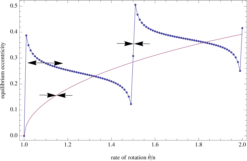
Figure 1: Equilibrium eccentricity (one corresponding to a vanishing average tidal torque) depicted against the dimensionless spin rate $\,\dot{\theta}/n\,$. Calculations were made for a tidally perturbed rotating body with parameters of the Moon, as shown in Table LABEL:table.                                                                                                                                  The monotonically rising curve corresponds to the linear torque (constant time lag) model. The jagged dotted line corresponds to a realistic rheology introduced in Section 4. Both functions were computed with a step of $\,0.01\,$ in $\,\dot{\theta}/n\,$.                                                                                                                                                                          In both cases, the resulting curve divides the plane into two parts corresponding to the two opposite signs of the average polar torque $\,\langle\,{\cal{T}}_{z}\,\rangle\,$. While $\,\langle\,{\cal{T}}_{z}\,\rangle\,$ is positive (accelerating) everywhere above the curve, it stays negative (decelerating) everywhere below the curve.                                                                                                                                                                         The small arrows indicate the action of the tidal torque upon small perturbations of the spin rate away from an equilibrium state. For the constant time lag model, the torque is restoring, and the equilibrium is stable. In the case of realistic rheology, though, the emerging nonzero torque drives the rotator away from the stable spin.

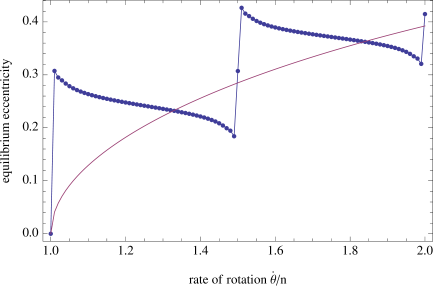
Figure 2: Equilibrium eccentricities of a zero secular tidal torque acting on a tidally perturbed super-Earth, depicted against the dimensionless spin rate $\,\dot{\theta}/n\,$. Parameters of the super-Earth are given in Table LABEL:table, and are consistent with those chosen for GJ581d in Makarov et al. (2012).                                                                                                                                  The monotonically rising curve represents the prediction of the constant time lag model.                                                                                                                                  The jigsaw dotted curve illustrates the prediction of the realistic rheological model described in Section 4. The function was computed for a grid of points at a step of $\,0.01\,$ in $\,\dot{\theta}/n\,$.

Within the constant time lag model, the function $\,e_{equ}(\dot{\theta}/n)\,$ being a smoothly rising curve explains the emergence of pseudosynchronism. To see this, consider a point on this curve, corresponding to a certain pseudosynchronous state. A small perturbation in $\,\dot{\theta}/n\,$ makes the tidally perturbed body rotate either faster or slower than the pseudosyncronous rate, and a nonzero tidal torque emerges. Illustrated by the two counter directed short arrows on the plot in Figure 1, the tidal torque is restoring, in that its action is opposite to the sign of perturbation. Thus, the tidal torque will return the perturbed rotator to the equilibrium state, i.e., to the initial position on the curve. So the equilibrium is stable.

The constant time lag model ignores the important contribution of rigidity (Segatz et al. 1988) and inelasticity (Karato and Spetzler 1990) into the tidal response of Earth-like planets. As a result, the model is incapable to account correctly for creep. As will be discussed in the following section, the above derivation of quasi-stable pseudosynchronism, from the linear torque model, is inapplicable to Earth-like planets with rigid mantles. However, in the viscous limit, this model may still be applicable to celestial bodies that do not have appreciable rigidity or inelasticity, such as gaseous planets and stars. Observations of binary stars, especially of short-period active stars on eccentric orbit, hold the best prospect of proving or disproving the linear torque model for this type of objects (Ferraz-Mello 2012, Torres et al. 2010).

The spin rate of active stars can be inferred from the characteristic periods of photometric variations caused by the passage of large spots or groups of spots across the visible disk of the star. The orbital period and the eccentricity are determined from spectroscopic radial velocity measurements. We find somewhat conflicting evidence for the existence of pseudosychronism in binary stars. Some stars with considerable eccentricities appear to have pseudosynchronous rotation (Hall 1986, Fekel et al. 1998), which is consistent with the original prediction by Hut (1981). Other stars clearly rotate faster or slower than the predicted rate (Fekel et al. 1993, Strassmeier et al. 2011). Even more puzzling, a significant number of tight binary systems have been found on circularised orbits, albeit spinning clearly asynchronously. This fact comes into contradiction with one of the important predictions of the linear torque theory, the one that synchronisation (or pseudosyncronisation) of rotation is achieved much sooner than circularisation (P. P. Eggleton 2011, private communication). Thus the impression created by the current body of observations is that the constant time lag model is, at least, not universally applicable to stars. This should not come as a surprise, because there exist theoretical indications that stars may have magnetic rigidity (Williams 2004, 2005, 2006; Ogilvie 2008, Garaud et al. 2010). 

Finally, it should be mentioned that, contrary to a common belief, the purely viscous model does not render a frequency-independent time lag at all frequencies. Stated differently, the purely viscous model does not imply that the factors $\,k_{l}(\omega_{lmpq})\,\sin\epsilon_{l}(\omega_{lmpq})\,$ are linear functions of the tidal mode $\,\omega_{lmpq}\,$ for all values of the mode. It can be demonstrated that this linearity takes place at low frequencies, but gets violated at frequencies higher than $\,G\rho^{2}R^{2}/\eta\,$, where $\,G$, $\,\rho$, $\,R$, and $\,\eta\,$ are the Newton gravity constant, mean density, radius, and the mean viscosity of the perturbed body. We shall address this topic elsewhere.

Table 1: Parameters of the tidal model.

Name	Description	Units	Values
			Moon	super-Earth
				( GJ581d )
$\xi$	moment of inertia coefficient		2/5	2/5
$R$	radius of the perturbed body	m	$1.737\times 10^{6}$	$1.083\times 10^{7}$
$M_{2}$	mass of the perturbed body	kg	$7.3477\times 10^{22}$	$4.23\times 10^{25}$
$M_{1}$	mass of the perturbing body	kg	$5.97\times 10^{24}$	$6.17\times 10^{29}$
$a$	semimajor axis	m	$3.84399\times 10^{8}$	$3.3\times 10^{10}$
$n$	mean motion, i.e. $2\pi/P_{\rm orb}$	yr-1	$84$	$34.25$
$e$	orbital eccentricity		0.0549	0.27
$(B-A)/C$	triaxiality		$2.278\times 10^{-4}$	$5\times 10^{-5}$
${G}$	gravitational constant	m3 kg-1 yr-2	$66468$	$66468$
$\tau_{M}$	Maxwell time	yr	5	50
$\mu$	unrelaxed rigidity modulus	Pa	$0.8\times 10^{11}$	$0.8\times 10^{11}$
$\alpha$	the Andrade parameter		$0.2$	$0.2$

4 Equilibrium torques for Earth-like planets and moons

To build a consistent theory of bodily tides, one has, first, to decompose the tide into a Fourier series and, second, to attribute to each Fourier component its own phase delay and magnitude decrease (the latter being expressed by the Love number appropriate to the said Fourier mode). Development of the decomposition technique was started by Darwin (1879) and accomplished in full by Kaula (1964). Attribution of phase delays and Love number values to the Fourier modes took much longer time, because of the necessity to explore rheological properties of the mantle at various frequencies. This exploration, by both seismological and geodetic methods, has been going on intensively through the past dozens of years. Merger of the Darwin-Kaula decomposition technique with the results from solid-Earth rheology is explained in Efroimsky (2012 a). The paper relied on a combined rheological model (Andrade at higher frequencies, Maxwell at lower frequencies), because of this model’s ability to best match laboratory experiments and both seismic and geodetic measurements of dissipation over a range of frequencies in the solid Earth. The merger of the Darwin-Kaula expansion with the combined rheological model, worked out in Ibid., has been used to predict spin-orbit resonances of a Mercury analogue having a constant eccentricity and a zero obliquity (Makarov 2012) and tidal properties of super-Earths (Efroimsky 2012 b).

4.1 Expression for the tidal torque

It is explained in Appendix A that the average polar component of the tidal torque can be approximated with the following expression, provided that (1) the obliquity is small, and (2) the perturbed body and the perturber are not too close to one another (so only the terms with degree-2 Love number are important) :

$$\langle\,{\cal{T}}_{z}\rangle_{\textstyle{{}_{{}_{\textstyle{{}_{l=2}}}}}}~{}=~{}\frac{3}{2}~{}\frac{\,G\,M_{1}^{\,2}}{a}\,\left(\frac{R}{a}\right)^{5}\sum_{q=-1}^{7}\,G^{\,2}_{\textstyle{{}_{\textstyle{{}_{20\mbox{\it{q}}}}}}}(e)~{}k_{2}(\omega_{\textstyle{{}_{\textstyle{{}_{220\mbox{\it{q}}}}}}})~{}\sin\epsilon_{2}(\omega_{\textstyle{{}_{\textstyle{{}_{220\mbox{\it{q}}}}}}})\,+O(e^{8}\,\epsilon)+O(i^{2}\,\epsilon)~{}=~{}\quad~{}\quad\quad$$ (8a)

$$\frac{3}{2}~{}\frac{\,G\,M_{1}^{\,2}}{a}\,\left(\frac{R}{a}\right)^{5}\sum_{q=-1}^{7}\,G^{\,2}_{\textstyle{{}_{\textstyle{{}_{20\mbox{\it{q}}}}}}}(e)~{}k_{2}(\omega_{\textstyle{{}_{\textstyle{{}_{220\mbox{\it{q}}}}}}})~{}\sin|\,\epsilon_{2}(\omega_{\textstyle{{}_{\textstyle{{}_{220\mbox{\it{q}}}}}}})\,|\,~{}\mbox{Sgn}\,\left(\,\omega_{220q}\,\right)+O(e^{8}\,\epsilon)+O(i^{2}\,\epsilon)~{}~{}.~{}\quad~{}$$ (8b)

This is the polar (orthogonal to the equator) component of the torque wherewith the tidally-perturbed body is acted upon by the perturber. The angular brackets denote orbital averaging, $\,G\,$ stands for the Newton gravitational constant, $\,M_{1}\,$ signifies the mass of the perturber (the star, if the perturbed body is its planet; or the planet, if the perturbed body is a satellite), $\,a\,$ is the semimajor axis, while $\,R\,$ is the radius of the tidally perturbed body. The degree-2 dynamical Love number $\,k_{2}\,$ and the phase lag $~{}\epsilon_{2}\,$ are functions of the Fourier tidal mode

$$\omega_{\textstyle{{}_{\textstyle{{}_{220\mbox{\it{q}}}}}}}\,=~{}(2~{}+~{}q)~{}n~{}-~{}2~{}\dot{\theta}\,~{}.$$ (9)

While the dynamical Love numbers $\,k_{2}(\omega_{\textstyle{{}_{220\mbox{\it{q}}}}})\,$ are positive definite, the sign of each phase lag $\,\epsilon_{2}(\omega_{\textstyle{{}_{220\mbox{\it{q}}}}})\,$ coincides with that of the Fourier mode $\,\omega_{\textstyle{{}_{220\mbox{\it{q}}}}}\,$, as can be understood from formulae (19) and (20) in Appendix A. It is for this reason that the products $\,k_{2}(\omega_{\textstyle{{}_{220\mbox{\it{q}}}}})\,\sin\epsilon_{2}(\omega_{\textstyle{{}_{220\mbox{\it{q}}}}})\,$ emerging in expression (8a) are rewritten in expression (8b) as $\,k_{2}(\omega_{\textstyle{{}_{220\mbox{\it{q}}}}})\,\sin|\,\epsilon_{2}(\omega_{\textstyle{{}_{220\mbox{\it{q}}}}})\,|~{}\,\mbox{Sgn}\,(\omega_{\textstyle{{}_{220\mbox{\it{q}}}}})\,$.

A generic expression for the torque implies summation over the four integer indices $~{}lmpq~{}$ serving to number the Fourier tidal modes $~{}\omega_{{\textstyle{{}_{lmpq}}}}~{}$ entering the spectrum – see Appendix A below. The terms of that series depend also upon the obliquity. As the $~{}lmpq~{}$ term contains a factor $\,(R/a)^{2l+1}\,$, it is often sufficient to keep only the degree-2 terms ($\,l=2\,$). In this case, with an extra assumption of small obliquity, it is enough to limit the summation to the terms with $\,m=2\,$, $\,p=0\,$. This renders expression (8).

While the full expression for the torque implies summation over all integer values of $\,q\,$, numerical tests demonstrate that, for eccentricities not exceeding $\,\sim\,0.3\,$, it is enough to take into account the terms up to $\,e^{7}\,$, inclusive. This would require summation from $\,q\,=\,-\,7\,$ through $\,q\,=\,7\,$. However, the values of the numerical factors entering the eccentricity polynomials $\,G_{\textstyle{{}_{\textstyle{{}_{20\mbox{\it{q}}}}}}}(e)\,$ are such that in practice it turns out to be sufficient to include only the terms with $\,q\,$ varying from $\,-\,1\,$ through $\,7\,$.

4.2 The tidal torque and the equilibrium eccentricity as functions of the spin rate

Expression (9) makes each product $\,k_{2}\,\sin\epsilon_{2}\,$ a function of the planetary spin rate $\,\stackrel{{\scriptstyle\bf\centerdot}}{{\theta~{}}}\,$:

$$k_{2}(\omega_{\textstyle{{}_{220\mbox{\it{q}}}}})\;\sin|\,\epsilon_{2}(\omega_{\textstyle{{}_{220\mbox{\it{q}}}}})\,|~{}\,\mbox{Sgn}\,(\,\omega_{\textstyle{{}_{220\mbox{\it{q}}}}}\,)~{}\quad\quad\quad\quad\quad\quad\quad\quad~{}\quad\quad\quad\quad\quad\quad\quad\quad\quad\quad\quad\quad~{}$$

$$=~{}k_{2}(\,2(n-\dot{\theta})\,+\,q\,n\,)~{}~{}\sin|\,\epsilon_{2}(\,2(n-\dot{\theta})\,+\,q\,n\,)\,|~{}~{}\mbox{Sgn}\,(\,2(n-\dot{\theta})\,+\,q\,n\,)\,~{}.~{}\quad$$ (10)

Consequently, the entire sum (8) can be treated as a function of $\,\stackrel{{\scriptstyle\bf\centerdot}}{{\theta\,}}$. The mean motion and eccentricity will play the role of parameters whose evolution is much slower than that of $\,\stackrel{{\scriptstyle\bf\centerdot}}{{\theta\,}}$.

Figure 3: Angular acceleration due to the secular tidal torque (8), in the vicinity of the 2:1 resonance. The dotted kink is the $\,q=2\,$ term which is an odd function when centered at $\dot{\theta}/n=1+q/2=2$. The solid line renders the total torque (8), i.e., a sum of the $q=2$ kink and the bias comprised by the terms with $q\neq 2$. Near the resonance, the bias is a slowly changing function of $\dot{\theta}/n$ and can be approximated with a constant. The $q=2$ kink resides on the right slope of a more powerful $q=1$ kink which is centered at $\dot{\theta}/n=1$ and dominates the bias. So the $q=2$ kink is shifted downward and goes through nil a tiny bit to the left of the resonance.                                                     The figure is borrowed from our work Makarov et al. (2012) devoted to the super-Earth GJ581d.

Each product $\,k_{2}\,\sin\epsilon_{2}\,$ is an odd function of the tidal mode $\,\omega_{220\mbox{\it{q}}}\,$ and has the shape of a kink centered around $\,\omega_{220\mbox{\it{q}}}=0\,$. When we employ relation (10) to write these products as functions of the spin rate, the new functions will still be kinks, though centered around $\,\dot{\theta}=n\left(1+{\textstyle q}/{\textstyle 2}\right)\,$. In Figure 3, the dotted line depicts the product

$$k_{2}(\omega_{\textstyle{{}_{\textstyle{{}_{2202}}}}})~{}\sin\epsilon_{2}(\omega_{\textstyle{{}_{\textstyle{{}_{2202}}}}})\,=\,k_{2}(\,4\,n\,-\,2\,\dot{\theta}\,)~{}\sin\epsilon_{2}(\,4\,n\,-\,2\,\dot{\theta}\,)$$

$$=~{}k_{2}(\,4\,n\,-\,2\,\dot{\theta}\,)~{}~{}\sin|\,\epsilon_{2}(\,4\,n\,-\,2\,\dot{\theta}\,)\,|~{}~{}\mbox{Sgn}\,(\,4\,n\,-\,2\,\dot{\theta}\,)\,~{}.$$ (11)

The kink shape of the $\,k_{2}\,\sin\epsilon_{2}\,$ products is determined by the rheological properties of the planet and its self-gravitation (see Appendix B for details and references). A kink transcends nil and changes sign continuously as the spin rate goes through the appropriate resonance.

In the sum (8), the kink-shaped products stand with multipliers $\,G^{\,2}_{\textstyle{{}_{\textstyle{{}_{20\mbox{\it{q}}}}}}}(e)\,$. So the overall tidal torque (8), as a function of $\,\dot{\theta}~{}$, is a superposition of many kinks having different magnitudes and centered at different resonances (nine kinks, if we sum over $\,q\,=\,-\,1,\,.\,.\,.\,7\,$). The ensuing curve will cross the horizontal axis in points extremely close to the resonances $\,\stackrel{{\scriptstyle\bf\centerdot}}{{\theta~{}}}=n\,\left(1+\,{\textstyle q}/{\textstyle 2}\right)\,$, but not exactly in these resonances — like the solid line in Figure 3.

4.3 The physical meaning of the kink

The physical forcing frequencies in the mantle, $\,\chi_{\textstyle{{}_{220\mbox{\it{q}}}}}\,$, are absolute values of the Fourier modes:

$$\chi_{\textstyle{{}_{220\mbox{\it{q}}}}}\,=~{}|\,\omega_{\textstyle{{}_{220\mbox{\it{q}}}}}\,|\,~{}.$$ (12)

The dynamical Love number is an even function of the tidal mode $\,\omega_{\textstyle{{}_{220\mbox{\it{q}}}}}\,$, while the phase lag is an odd function. For this reason, the product $\,k_{2}(\omega_{\textstyle{{}_{220\mbox{\it{q}}}}})\,\sin\epsilon_{l}(\omega_{\textstyle{{}_{220\mbox{\it{q}}}}})\,$ can be rewritten as a function of the physical frequency $\,\chi\,$, multiplied by the sign of the appropriate Fourier mode:

$$k_{2}(\omega_{\textstyle{{}_{220\mbox{\it{q}}}}})\,\sin\epsilon_{l}(\omega_{\textstyle{{}_{220\mbox{\it{q}}}}})\,=~{}k_{2}(\chi_{\textstyle{{}_{220\mbox{\it{q}}}}})\,\sin|\epsilon_{2}(\chi_{\textstyle{{}_{220\mbox{\it{q}}}}})|\,{\mbox{Sgn}}\,(\omega_{\textstyle{{}_{220\mbox{\it{q}}}}})\,~{}.$$ (13)

Outside the inter-peak interval (i.e., at frequencies that are not too low), the positive definite quantity $~{}k_{2}(\chi)\,\sin|\epsilon_{2}(\chi)|\,$ is decreasing monotonically with increase of the frequency $\,\chi=\chi_{\textstyle{{}_{220\mbox{\it{q}}}}}\,$. This happens for two reasons. One, intuitively obvious, is that the dynamical Love number decreases at higher frequencies, because materials are inertial, and it is getting harder for their shape to keep up with the varying stress as the frequency goes up. Less obvious is the circumstance that the sine of the phase lag (i.e., the inverse tidal quality factor), too, decreases as the frequency grows. Supported by a mighty volume of seismological, geodetic, and laboratory data, this behaviour may look counterintuitive because this is not what one would expect from a viscous fluid. The fact however is that at physically interesting frequencies the mantle behaves itself not as a viscous or a Kelvin-Vogt body but as an Andrade body dissipation wherein obeys the law $\,\sin\epsilon\propto\chi^{\,-\,\alpha}\,$, with $\,\alpha\approx 0.14-0.4\,$ for most solids (Efroimsky 2012a, 2012b).

Finally, the steep (but still continuous) near-resonant jumps connecting the peaks of the kink are explained by the fact that at those locations self-gravitation “beats” rheology (Ibid.).

The kink shape of $\,k_{2}\,\sin\epsilon_{2}\,$ (generally, of $\,k_{l}\,\sin\epsilon_{l}\,$) entails somewhat counterintuitive consequences for the phase lag and the geometric lag angle. Consider the principal, semidiurnal bulge. Its phase lag and the geometric lag angle are

$$\epsilon_{2}(\omega_{\textstyle{{}_{\textstyle{{}_{2200}}}}})\,=\,\omega_{\textstyle{{}_{2200}}}~{}\Delta t_{2}(\omega_{\textstyle{{}_{\textstyle{{}_{2200}}}}})\,=\,2\,(n\,-\,\dot{\theta})~{}\Delta t_{2}(\omega_{\textstyle{{}_{\textstyle{{}_{2200}}}}})\,$$ (14)

and

$$\delta_{2}(\omega_{\textstyle{{}_{2200}}})~{}=~{}\frac{1}{2}~{}|\,\epsilon_{2}(\omega_{\textstyle{{}_{2200}}})\,|\,=\,|\,n\,-\,\dot{\theta}\,|~{}\Delta t_{2}(\omega_{\textstyle{{}_{\textstyle{{}_{2200}}}}})\,~{}.$$ (15)

Were a planet composed of a material with the time lag $\,\Delta t_{2}(\omega_{\textstyle{{}_{\textstyle{{}_{2200}}}}})\,$ insensitive to the value of the principal tidal mode $\,\omega_{\textstyle{{}_{2200}}}\,=\,2\,|n\,-\,\dot{\theta}|\,$, the geometric lag angle would be larger for a higher value of this frequency. This indeed is what one would, intuitively, expect: the higher the difference between $\,\dot{\theta}\,$ and $\,n\,$ the larger the angle. However, for a realistic rheology, an increase of the $\,\delta_{\textstyle{{}_{2200}}}\,$ angle due to an increase in $\,2\,|n\,-\,\dot{\theta}|~{}$ will take place only within an extremely close proximity of the the $\,1:1\,$ resonance. Stepping beyond the kink’s peak, we shall find that an increase in $\,2\,|n\,-\,\dot{\theta}|~{}$ will be accompanied by such a decrease in the time lag $\,\Delta t_{2}(\omega_{\textstyle{{}_{\textstyle{{}_{2200}}}}})\,$ that the product of these two quantities will, overall, be decreasing with growing frequency. So both the phase lag and the geometric lag angle will become smaller.

4.4 Instability of pseudosynchronous rotation. Physical interpretation

Since the mode-dependence of the products (10) follows from the rheological properties of the mantle and from self-gravitation of the planet, these products turn out to be functions not only of the tidal mode $\omega_{\textstyle{{}_{220\mbox{\it{q}}}}}\,$, but also of the parameters defining the size and rheology of the perturbed body. These parameters (presented in Table 1) are the body’s radius $\,R\,$ and mass $\,M_{2}\,$, as well as its unrelaxed rigidity $\,\mu\,$, Maxwell time $\,\tau_{M}\,$, inelastic (Andrade) time $\,\tau_{A}\,$, and the Andrade parameter $\,\alpha\,$.

For a given selection of these parameters’ values and a fixed spin rate $\,\dot{\theta}\,$, there is a unique eccentricity $\,e_{\rm equ}\,$ at which $~{}\langle\,{\cal{T}}_{z}\rangle_{\textstyle{{}_{{}_{\textstyle{{}_{l=2}}}}}}=0\,$. The dependence of $\,e_{\rm equ}\,$ on the relative rate of rotation $\,\dot{\theta}/n\,$ can be found for a grid of points by numerically determining the roots of $~{}\langle\,{\cal{T}}_{z}\rangle_{\textstyle{{}_{{}_{\textstyle{{}_{l=2}}}}}}~{}$ in $\,e\,$. To accomplish this, we recall that each term in Equation (8) is a polynomial in $\,e\,$ and, therefore, so is the entire right-hand side of (8). Computational search of the roots was carried out for two sets of parameters listed in Table 1, one representing the Moon orbiting the Earth, and the other a hypothetical super-Earth orbiting a solar analog. The choice of parameters is intended to represent the range of applicability of the model. The resulting dependencies of $\,e_{\rm equ}\,$ upon $\,\dot{\theta}/n\,$ are presented in Figures 1 and 2.

The jigsaw shape of the found dependencies $\,e_{\rm equ}(\dot{\theta}/n)\,$ is remarkably different from the predictions of the linear torque model. The curves for the Moon (Figure 1) and the super-Earth (Figure 2) are monotonically descending with a rising rate of rotation, everywhere between the spin-orbit resonances. This has profound implications for the character of equilibrium at a zero tidal torque. Consider an arbitrary point on the downhill portion of the curve, e.g., the one in Figure 1, from which two short arrows of opposite direction are drawn. A perturbation in $\,\dot{\theta}\,$ away from this point, whether spinning the planet up or slowing it down, will cause a nonzero tidal torque acting in the same direction – as indicated by the direction of the arrows. Thereby, the tidal equilibrium achieved at $\,e_{\rm equ}\,$ between the resonances is inherently unstable. Similarly, a perturbation in $\,e\,$ will make the planet diverge from the curve of zero torque rather than return to it. Hence, the states of zero tidal torque at non-resonant spin rates are transient by nature.

In a narrow vicinity of each spin-orbit resonance, $\,e_{\rm equ}\,$ takes a rapid upward increase. Computation of the roots of Equation 8 is numerically difficult in these areas because of a very large gradient of the curve. The slope of the segments at the resonances is positive; therefore, there exists a stable equilibrium just as in the case of the linear torque model. A deviation of the spin rate from a resonant value gives rise to a nonzero restoring torque, as indicated by a pair of inward arrows in Figure 1 at the resonance 3:2.

To obtain a physical explanation of the unstable nature of the pseudosynchronous rotation, recall two circumstances. First, each term of the sum (8) has the shape of a kink. Second, each such kink, as a function of $\,\dot{\theta}\,$, is increasing monotonically everywhere except near the appropriate resonance, as in Figure 3. For this reason, an infinitesimal increase in $\,\dot{\theta}/n\,$ furnishes an infinitesimal increase in the tidal torque (not necessarily in its absolute value). This happens for an arbitrary value of $\,e\,$ and for the values of $\,\dot{\theta}/n\,$ outside the narrow resonances. Specifically, for $\,e=e_{equ}\,$, the torque is zero and acquires a positive value, which leads to further spin-up. The spin-up continues until $\,\dot{\theta}/n\,$ stumbles into a resonance. (Resonances are depicted with near-vertical segments of the dotted curves in Figures 1 and 2.)

4.5 On the choice of the values for physical parameters

Figures 1 and 2 reveal, in comparison, that the structure of the equilibrium tidal torque is similar for a wide range of values of planetary parameters. The values employed to build these plots are shown in Table LABEL:table. The rapid jumps of $\,e_{\rm equ}\,$ at resonances and the smooth descents between the resonances are characteristic of small moons and large planets likewise. The values of $\,e_{\rm equ}\,$ at resonances appear to be the same for the Moon and the model super-Earth. The most noticeable difference is in the amplitude of the resonance jumps, which is significantly higher for the Moon. By experimenting with the input parameters, we found out that this amplitude is sensitive mainly to the Maxwell time $\,\tau_{M}\,$, which differs by an order of magnitude between our model bodies.

The choice of such a small Maxwell time for the Moon, only 5 years, is justified by the likely presence of a high percentage of partial melt in the lower lunar mantle. The presence of partial melt follows from the modeling carried out by Weber et al. (2011) and also from an earlier study by Nakamura et al. (1974). There exists data pointing at the possibility of the lunar Maxwell time being of the order of months.

The choice of the parameters of the super-Earth was consistent with that made in Makarov et al. (2012) for the planet GJ581d.

The Arrhenius law requires that planets and moons with hotter interiors have lower viscosity of mantles and, thus, have shorter Maxwell times. So we surmise that the secular tidal torque for such objects should be relatively more efficient in capturing at higher spin-orbit resonances.

5 Resonant rotation of axisymmetric bodies

We have determined that a stable spin-orbit equilibrium is achieved at spin rates where the value of the secular polar tidal torque is zero, while the derivative of the equilibrium eccentricity with respect to the spin rate, $~{}{\textstyle de_{equ}}/{\textstyle d(\dot{\theta}/n)}~{}$, is negative. With the realistic tidal model discussed in Appendix B, this may happen only in the vicinity of spin-orbit resonances because the derivative of the torque is positive elsewhere. The secular torque (8), as well as the angular acceleration caused by it, has “kinks” in the vicinity of spin-orbit commensurabilities $\,\dot{\theta}/n\,=\,1\,+\,q/2~{}$, with an integer $\,q\,$ of either sign. An example thereof is shown in Figure 4 for the super-Earth model, within a segment of the spin rate around $\,\dot{\theta}/n=5/2\,$. The kink is comprised by a local maximum below the resonance and a minimum above the resonance.

To understand the plot in Figure 4, recall that in the vicinity of each resonance $\,q\,^{\prime}\,$, i.e., for $\,\dot{\theta}/n\,$ being close to $~{}1\,+\,{\textstyle q\,^{\prime}}/{\textstyle 2}~{}$, the right-hand side of (8) can be decomposed into two parts. One part is the $\,q=q\,^{\prime}\,$ term. It is a kink-looking odd function of the tidal mode $\,\omega_{220q}\,$, and it goes through nil at exactly $\,\omega_{220q}=0~{}$. Due to (9), this term can also be interpreted as a function of the spin rate, antisymmetric with respect to the resonance point $\,\dot{\theta}/n\,=\,1\,+\,{\textstyle q\,^{\prime}}/{\textstyle 2}\,$ where this term goes through nil. The second part, called bias, is the rest of the sum, i.e., the input of all the $\,q\neq q\,^{\prime}\,$ Fourier modes into the values assumed by the torque in the vicinity of the $\,q=q\,^{\prime}\,$ resonance. The bias can be negative or positive in value, depending on the eccentricity. For not too large eccentricities, it is usually negative. Being a very slowly changing function within the resonance interval, it can, to a good approximation, be assumed constant there.

Having summed up all the terms in (8), and exploring the behaviour of this sum near $\,\dot{\theta}/n\,=\,1\,+\,{\textstyle q\,^{\prime}}/{\textstyle 2}\,$, we see that the resulting curve does not cross the horizontal axis at $\,\dot{\theta}/n\,=\,1\,+\,{\textstyle q\,^{\prime}}/{\textstyle 2}\,$. One can say that the bias slightly displaces the location of zeros. The zeros are located close to resonances but not exactly in resonances.

In Figure 4(a), the values of the overall torque (in fact, of the total angular acceleration proportional to the torque) are defined mostly by the $\,q=3\,$ term which, in this vicinity, looks like an antisymmetric kink. However, the curve is shifted down due to the bias which is defined mainly by the right slope of the $\,q=1\,$ kink located to the left. Since the right slope of the $\,q=1\,$ kink is negative, the $\,q=3\,$ kink is shifted down. As a result, the maximum secular torque barely rises above zero, and the curve has two zeros located to the left of the point $\,\dot{\theta}/n\,=\,5/2\,$, close to the maximum of the kink. The interval of the resonance is defined by the location of the peaks: $\,\dot{\theta}/n=2.4998\,$ and $\,2.5002\,$.

Figure 4(b) is a blow-up of Figure 4(a) showing in greater detail the area around the maximum of the kink. The root of the function within the resonance interval is at $\,2.49985\,$ rather than exactly $\,2.5\,$. For the same reason, the torque value is negative at $\,\dot{\theta}/n=2.5\,$.

In the framework of this model, it is reasonable to define capture in resonance as an equilibrium state in which the body’s average rotation rate stays between the values corresponding to these two peaks. This definition is adequate because, as we saw above, stable equilibrium is possible only on negative slopes of the angular acceleration (or tidal torque) as a function of the spin rate.

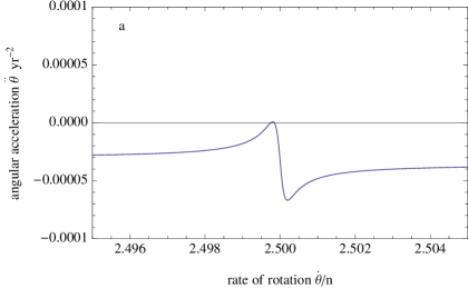
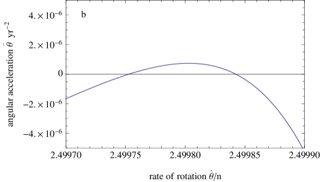
Figure 4: Angular acceleration of the super-earth (Table 1) caused by the secular tidal torque in the vicinity of the 5:2 resonance, (a) showing the entire resonance interval, and (b) showing in more detail the same curve in the area of the local maximum.

When a triaxial planet is captured in a 5:2 resonance, its time-averaged spin rate is exactly $\,2.5\,n\,$. Similarly, the Moon’s spin rate, captured in synchronous rotation, is exactly $\,1\,n\,$. However, we know that the time-averaged tidal torque is nonzero at this spin rate. Why does not the Moon accelerate? For a triaxial body, the nonzero secular tidal torque is compensated by a counteracting triaxiality-caused torque, through a small tilt of the average inertia axis with respect to the line connecting the centres of the bodies. A nonzero time-average tilt generates a secular triaxial torque. This mechanism of torque compensation obviously does not work for the rather hypothetical case of axisymmetric body, which would be subject to only tidal forces. Would the Moon be facing the Earth always with the same side if it were completely axisymmetric? First, we have to find out if capture in spin-orbit resonance is at all possible. The answer is yes, as long as the secular torque changes sign in the vicinity of that resonance . Even though the maximum torque in Figure 4 barely rises above zero at spin rates below the resonance, it turns out to be sufficient for capture in 5:2. Figure 5 displays the results of a numerical integration of the evolution of spin rate for the super-Earth model (Table 1) at $\,\tau_{M}=50$ yr with an initial spin rate of $\,\dot{\theta}(0)=2.51\,n\,$. The planet is captured in about 8500 yr, but the equilibrium spin rate at $\,2.49985\,n\,$ is clearly below the resonance value. This value is consistent with the root of the secular torque within the resonance interval, Figure 4(b). Thus, the equilibrium resonance state of an axisymmetric body is achieved at the spin rate where the secular tidal torque equals zero, as expected.

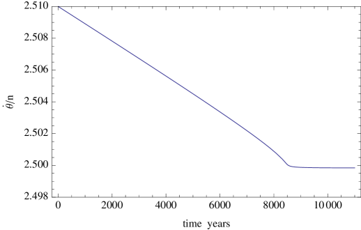
Figure 5: Capture of an axisymmetric super-Earth (Table 1, but with $(B-A)/C=0$) in 5:2 resonance. Note that the ultimate equilibrium spin rate is slightly less than $2.5\,n$.

6 Word of caution

As was demonstrated above, stability of pseudosynchronous spin hinges upon rheology. Being stable for the constant time lag model, the regime is expected to be transient for realistic mantles, insofar as their $\,k_{2}(\chi)\,\sin\epsilon_{2}(\chi)\,$ has one pronounced peak (not to count the opposite one at the negative value of the tidal mode) – see Figure 3. The situation will have to be re-analysed for bodies of complex structure (with surface or internal oceans), as well as for bodies of yet unexplored rheologies. Specifically, if it happens that somewhere in universe there exist bodies with not one but two pronounced peaks of $\,k_{2}\,\sin\epsilon_{2}\,$ at positive frequencies, the “ditch” between these peaks may, in principle, lead to emergence of a pseudosynchronous rotation state. Such a peak may emerge at the boundary of two frequency bands dominated by different friction mechanisms, i.e., when a new mechanism is “turned on” very quickly with the increase of frequency. Although highly hypothetical, such situations should not be written off completely.

7 Discussion

The shortness of Earth’s day was undoubtedly beneficial for proliferation of biological life, making the daily temperature variation moderate. The situation may be drastically different for the growing class of potentially habitable super-Earth exoplanets. Due to the observational selection effect, the spectroscopically detected super-Earths are found mostly around lower-mass stars, whose habitable zones are inevitably narrower and closer. For such systems, any conclusion about potential habitability of a given exoplanet becomes especially uncertain, and the analysis becomes intricately involved with regard to such parameters as the amount of stellar irradiation, the chemical composition of a hypothetical atmosphere, and the internal heating. The rate of rotation is also a crucial parameter which for now remains unavailable from observation. The most advanced climatic simulations are based on a certain assumption of the spin-orbit state of the planet, e.g., a tidal synchronisation (1:1 resonance) is assumed, as in Selsis et al (2011). A tidally synchronised planet showing the same side to its host star has this side always exposed to plentiful irradiation, the other side staying dark. Such planets can hardly retain an atmosphere and can hardly be habitable. However, a spin-orbit locking into higher commensurabilities (e.g., 3:2, as in the case of Mercury) allows the planet to rotate with respect to the host star, and leaves the planet a possibility of sustaining a stable atmosphere and having water in the liquid form on the surface. Three-dimensional climatic simulations of the potentially habitable super-Earth GJ 581d, by Wordsworth et al. (2010), were performed for a set of possible spin-orbit resonances, including 2:1. As was later explained in Makarov et al. (2012), this resonance is the likeliest state of GJ 581d for a wide range of rheological parameters, assuming a terrestrial composition of its mantle. Wordsworth et al. (2010) drew attention to the fact that a tidally synchronised atmosphere may be short-lived because of the collapse of CO₂ on the night side. A similar phenomenon may occur on a slowly rotating planet. Both the constant angular lag tidal model and the constant time lag model predict that oblate planets with moderate and large eccentricities are captured in stable pseudosynchronous rotations, in which case their spin rate only slightly exceeds their orbital mean motion. This would make an entire class of detected exoplanets unsuitable for biological life. In this paper we prove that the prediction of pseudo-synchronism is germane to the above-mentioned simplified models of tidal interactions, models inapplicable to solid planets or moons. Super-Earth exoplanets of Earth-like composition on eccentric orbits are likely to be captured into spin-orbit resonances higher than 1:1, but there is no such thing as pseudo-synchronous rotation for these objects.

Appendix  A.      The tidal torque                

The additional potential $\,U\,$ of a tidally perturbed body can be expanded into a Fourier series over the tidal modes

$$\omega_{lmpq}\;\equiv\;({\it l}-2p)\;\dot{\omega}\,+\,({\it l}-2p+q)\;{\bf{\dot{\cal{M}}}}\,+\,m\;(\dot{\Omega}\,-\,\dot{\theta})\,\approx\,(l-2p+q)\,n\,-\,m\,\dot{\theta}\,~{},~{}~{}~{}$$ (16)

where $\,{\theta}\,$ and $\,\dot{\theta}\,$ are the sidereal angle and rotation rate of the body, while $\,\omega\,$, $\,\Omega\,$, $\,n\,$, and $\,{\cal{M}}\,$ are the periapse, the node, the mean motion, and the mean anomaly of the perturber as seen from the perturbed body.

While the tidal modes $\,\omega_{\textstyle{{}_{lmpq}}}\,$ can be of either sign, the forcing frequencies

$$\chi_{lmpq}\,=~{}|\,\omega_{lmpq}\,|~{}\approx~{}|~{}(l-2p+q)~{}n\,-\,m~{}\dot{\theta}~{}|$$ (17)

at which the strain and stress oscillate are positive-definite.

The series expansion of the additional potential $\,U\,$ was developed by Kaula (1964), its partial sum known yet to Darwin (1879). Therefore the series for $\,U\,$ and the resulting series for the torque are often named the Darwin-Kaula expansions.

An accurate derivation of the expansion for the torque demonstrates that the torque contains both a rapidly oscillating and a secular part (Efroimsky 2012a). Having a zero orbital average, the oscillating part nevertheless may play a role in dissipation of free librations. In Makarov et al. (2012) it was explored whether the oscillating part of the torque can influence capture into resonances. Changing the outcome of a particular realisation of the capture scenario, the oscillating part did not alter the statistics.

The secular part of the polar torque looks as

$$\langle\,{\cal{T}}_{z}\rangle\,=\,2\,G\,M_{star}^{{{\,2}}}\sum_{{\it{l}}=2}^{\infty}\frac{R^{\textstyle{{}^{2l\,+\,1}}}}{a^{\textstyle{{}^{2l\,+\,2}}}}\sum_{m=0}^{l}\frac{(l-m)!}{(l+m)!}\;m\sum_{p=0}^{l}F^{\,2}_{lmp}(i)\sum^{\it\infty}_{q=-\infty}G^{\,2}_{lpq}(e)\;k_{l}(\omega_{lmpq})\;\sin\epsilon_{l}(\omega_{lmpq})\,~{},\quad$$ (18)

where the angular brackets signify orbital averaging, $\,G\,$ denotes Newton’s gravity constant, $\,a,\,i,\,e\,$ are the semimajor axis, inclination (or obliquity), and eccentricity, while $\,F_{lmp}(i)\,$ and $\,G_{lpq}(e)\,$ are the inclination functions and eccentricity polynomials. The Love numbers $\,k_{\textstyle{{}_{l}}}\,$ and the phase lags $\,\epsilon_{\textstyle{{}_{l}}}\,$ depend on the modes (16).

In the Darwin-Kaula theory, the phase lags come into being as products of the modes $\,\omega_{lmpq}\,$ by the corresponding time delays:

$$\epsilon_{l}(\omega_{lmpq})\,=\,\omega_{lmpq}~{}\,\Delta t_{l}(\omega_{lmpq})\,~{},$$ (19)

where, for causality reasons, the time lags $\,\Delta t_{\textstyle{{}_{l}}}(\omega_{\textstyle{{}_{lmpq}}})\,$ are positive-definite. Therefore, (19) may be rewritten as

$$\epsilon_{l}(\omega_{lmpq})\,=\,\chi_{lmpq}~{}\,\Delta t_{l}(\omega_{lmpq})~{}\,\mbox{Sgn}\,(\,\omega_{lmpq}\,)\,~{},$$ (20)

$\chi_{lmpq}\,$ being the physical forcing frequencies (17). As a result of this, the entire expression for the polar component of the torque can be written down as

$$\langle\,{\cal{T}}_{z}\rangle\,=~{}~{}~{}\quad~{}\quad~{}\quad~{}\quad~{}~{}\quad~{}\quad~{}\quad~{}\quad~{}\quad~{}\quad~{}\quad~{}\quad~{}\quad~{}\quad~{}\quad~{}\quad~{}\quad~{}\quad~{}\quad~{}\quad~{}\quad~{}\quad~{}\quad~{}\quad~{}\quad~{}\quad~{}\quad~{}\quad$$

$$2\,GM_{star}^{{{\,2}}}\sum_{{\it{l}}=2}^{\infty}\frac{R^{\textstyle{{}^{2l\,+\,1}}}}{a^{\textstyle{{}^{2l\,+\,2}}}}\sum_{m=0}^{l}\frac{(l-m)!}{(l+m)!}\;m\sum_{p=0}^{l}F^{\,2}_{lmp}(i)\sum^{\it\infty}_{q=-\infty}G^{\,2}_{lpq}(e)\;k_{l}(\omega_{lmpq})~{}\sin|\,\epsilon_{l}(\omega_{lmpq})\,|\,~{}\mbox{Sgn}\,\left(\,\omega_{lmpq}\,\right)\,~{}.\quad$$ (21)

Be mindful that, similar to the Love numbers, we prefer to denote the lags with $\,\epsilon_{l}(\omega_{lmpq})\,$ and $\,\Delta t_{l}(\omega_{lmpq})\,$, and not with $\,\epsilon_{lmpq}\,$ and $\,\Delta t_{lmpq}\,$.

When the bodies are not too close (${\textstyle R}/{\textstyle a}\ll 1$), we drop the terms with $\,l>2\,$. For small obliquities ($i\simeq 0$), we leave only $\,i-$independent terms (the next-order terms being quadratic in $\,i\,$). Finally, for eccentricities not exceeding $\,\sim\,0.3\,$, only the terms up to $\,e^{7}\,$ are important. Formally, this would imply summation over $\,q\,=\,-\,7,\,.\,.\,.7\,$. However, the term with $\,q\,=\,-\,2\,$ vanishes identically, while those with $\,q\,=\,-\,7,\,.\,.\,.\,-\,3\,$ are accompanied with extremely small numerical factors and can thus be dropped. So the polar component of the torque is approximated with

$$\langle\,{\cal{T}}_{z}\rangle_{\textstyle{{}_{{}_{\textstyle{{}_{l=2}}}}}}~{}=~{}~{}\quad~{}\quad~{}~{}\quad~{}\quad~{}\quad~{}\quad~{}\quad~{}\quad~{}\quad~{}\quad~{}\quad~{}\quad~{}\quad~{}\quad~{}\quad~{}\quad~{}\quad~{}\quad~{}\quad~{}\quad~{}\quad~{}\quad~{}\quad~{}\quad~{}\quad~{}\quad$$

$$\frac{3}{2}~{}G\,M_{star}^{\,2}\,R^{5}\,a^{-6}\sum_{q=-1}^{7}\,G^{\,2}_{\textstyle{{}_{\textstyle{{}_{20\mbox{\it{q}}}}}}}(e)~{}k_{2}(\omega_{\textstyle{{}_{\textstyle{{}_{220\mbox{\it{q}}}}}}})~{}\sin|\,\epsilon_{2}(\omega_{\textstyle{{}_{\textstyle{{}_{220\mbox{\it{q}}}}}}})\,|\,~{}\mbox{Sgn}\,\left(\,\omega_{220q}\,\right)+O(e^{8}\,\epsilon)+O(i^{2}\,\epsilon)~{}~{},~{}\quad~{}\quad~{}$$ (22)

For the first time, this expression (with a sum running over all integer $\,q\,=\,-\,\infty,\,.\,.\,.\,\infty\,$) was written, with no proof, by Goldreich & Peale (1966). A sketch of a proof was later suggested by Dobrovolskis (2007).

The functional form of the dependence of the factors $~{}k_{l}\,\sin\epsilon_{l}~{}$ upon the mode $\,\omega_{\textstyle{{}_{lmpq}}}\,$ is determined by the size and mass of the body and by its rheological properties. By rheology we imply the so-called constitutive equation of the medium, i.e., an equation interconnecting the strain and stress. For linear deformations, such equations can be rewritten in the frequency domain where each harmonic mode of the strain becomes expressed algebraically through the appropriate harmonic mode of the stress. Using the method explained in Efroimsky (2012a, 2012b), the algebraic relations can be used to find the shape of the functions $\,k_{l}(\omega_{\textstyle{{}_{lmpq}}})~{}\sin\epsilon_{l}(\omega_{\textstyle{{}_{lmpq}}})\,$ standing in the terms of the Darwin-Kaula expansion of the tidal torque.

Calculations of the shapes of these functions, presented in Ibid., are based on a combined rheological model (Andrade at higher frequencies, Maxwell at lower frequencies), because of this model’s ability to best match laboratory experiments and both seismic and geodetic measurements of dissipation over a broad range of frequencies in the solid Earth. It is reasonable to assume that the model is applicable to the mantles of other terrestrial planets and moons. As demonstrated in Ibid., this combined model furnishes for $\,k_{l}~{}\sin\epsilon_{l}\,$ a kink-shaped dependence upon the Fourier mode – as in Figure 4.

Appendix  B.     Calculation of the factors $~{}k_{l}(\omega_{\textstyle{{}_{lmpq}}})~{}\sin\epsilon_{l}(\omega_{\textstyle{{}_{lmpq}}})~{}$

As explained in Efroimsky (2012a, 2012b), the products $~{}k_{l}(\omega_{\textstyle{{}_{lmpq}}})~{}\sin\epsilon_{l}(\omega_{\textstyle{{}_{lmpq}}})~{}$ can be expressed through the mass and radius of the planet, and the real and imaginary parts of the complex compliance of its mantle. Thereby, the shape of the functional dependence of $~{}k_{l}~{}\sin\epsilon_{l}~{}$ upon $\,\omega_{\textstyle{{}_{lmpq}}}\,$ is defined by both the self-gravitation of the planet and its rheological properties. The functions turn out to be odd. They go continuously through nil, changing their sign, when the argument $\,\omega_{\textstyle{{}_{lmpq}}}\,$ goes through nil, i.e., when a commensurability is crossed.

These odd functions can then be written down as $~{}k_{l}(\omega_{\textstyle{{}_{lmpq}}})~{}\sin|\,\epsilon_{l}(\omega_{\textstyle{{}_{lmpq}}})\,|~{}\,\mbox{Sgn}\,(\,\omega_{\textstyle{{}_{lmpq}}}\,)~{}$. Here the product $~{}k_{l}(\omega_{\textstyle{{}_{lmpq}}})~{}\sin|\,\epsilon_{l}(\omega_{\textstyle{{}_{lmpq}}})\,|~{}$ is an  even  function of the tidal mode and can thus be treated as a function not of the tidal mode $\,\omega_{\textstyle{{}_{lmpq}}}\,$ but of its absolute value $\,\chi_{\textstyle{{}_{lmpq}}}\,=\,|\,\omega_{\textstyle{{}_{lmpq}}}\,|\,$, which is the actual frequency of the oscillating stress in the mantle:

$$k_{l}(\omega_{\textstyle{{}_{lmpq}}})~{}\sin\epsilon_{l}(\omega_{\textstyle{{}_{lmpq}}}) = k_{l}(\omega_{\textstyle{{}_{lmpq}}})~{}\sin|\,\epsilon_{l}(\omega_{\textstyle{{}_{lmpq}}})\,|~{}\,\mbox{Sgn}\,(\,\omega_{\textstyle{{}_{lmpq}}}\,)$$ (23)

$$= k_{l}(\chi_{\textstyle{{}_{lmpq}}})~{}\sin|\,\epsilon_{l}(\chi_{\textstyle{{}_{lmpq}}})\,|~{}\,\mbox{Sgn}\,(\,\omega_{\textstyle{{}_{lmpq}}}\,)\,~{}.$$

The development in Ibid. results in the following frequency dependence:

$$k_{l}(\omega_{\textstyle{{}_{lmpq}}})\;\sin\epsilon_{l}(\omega_{\textstyle{{}_{lmpq}}})\,=\;\frac{3}{2\,({\it l}\,-\,1)}\;\,\frac{-\;A_{l}\;J\;{\cal{I}}{\it{m}}\left[\bar{J}(\chi)\right]}{\left(\;{\cal{R}}{\it{e}}\left[\bar{J}(\chi)\right]\;+\;A_{l}\;J\;\right)^{2}\;+\;\left(\;{\cal{I}}{\it{m}}\left[\bar{J}(\chi)\right]\;\right)^{2}}~{}\,\mbox{Sgn}\,(\,\omega_{\textstyle{{}_{lmpq}}}\,)~{}~{}~{},~{}~{}~{}~{}~{}$$ (24)

where $\,\chi\,$ is a shortened notation for the frequency $\,\chi_{\textstyle{{}_{lmpq}}}\,$, while coefficients $\,A_{l}\,$ are given by

$$A_{\it l}\,\equiv\;\frac{\textstyle{(2\,{\it{l}}^{\,2}\,+\,4\,{\it{l}}\,+\,3)\,{\mu}}}{\textstyle{{\it{l}}\,\mbox{g}\,\rho\,R}}\;=\;\frac{\textstyle{3\;(2\,{\it{l}}^{\,2}\,+\,4\,{\it{l}}\,+\,3)\,{\mu}}}{\textstyle{4\;{\it{l}}\,\pi\,G\,\rho^{2}\,R^{2}}}\;\;\;.~{}~{}~{}~{}~{}~{}~{}$$ (25)

with $\,G\,$ being the Newton gravitational constant, and $\,R\,$, $\,\rho\,$, $\,\mu\,$, and g being the radius, mean density, unrelaxed rigidity, and surface gravity of the planet. The functions

$${\cal R}{\it e}[\bar{J}(\chi)]\;=\;J\;+\;J\,(\chi\tau_{{}_{A}})^{-\alpha}\;\cos\left(\,\frac{\alpha\,\pi}{2}\,\right)\;\Gamma(\alpha\,+\,1)~{}~{}~{}~{}\quad\quad\quad\quad\quad~{}\quad\quad\quad\quad\quad\quad\quad$$ (26)

and

$${\cal I}{\it m}[\bar{J}(\chi)]\;=\;-\;J~{}(\chi\tau_{{}_{M}})^{-1}\;-\;J\,(\chi\tau_{{}_{A}})^{-\alpha}\;\sin\left(\,\frac{\alpha\,\pi}{2}\,\right)\;\Gamma(\alpha\,+\,1)~{}~{}~{}~{}~{}~{}~{}~{}~{}~{}~{}~{}~{}~{}~{}~{}~{}~{}\quad\quad\quad$$ (27)

are the real and imaginary parts of the complex compliance $\,\bar{J}(\chi)\,$ of the mantle. Here $\,\alpha\,$ is the Andrade parameter assuming values of about $\,0.3\,$ for solid silicates and about $\,0.14-0.2\,$ for partial melts. In our computations, we used $\,\alpha=0.2\,$. The quantity $\,J\,$ is the unrelaxed compliance of the mantle, which is the inverse of the mantle’s unrelaxed rigidity $\,\mu\,$. The parameters $\,\tau_{{}_{M}}\,$ and $\,\tau_{{}_{A}}\,$ are typical timescale characterising the mantle’s viscoelastic and inelastic response, correspondingly.

The Maxwell time $\,\tau_{{}_{M}}\,$ is the ratio of the mantle’s viscosity $\,\eta\,$ to its rigidity $\,\mu\,$. While for the Earth’s mantle it has a value of about 500 years, it may be much shorter for warmer planets and moons due to the exponential temperature-dependence of the viscosity.

The inelastic (Andrade) time $\,\tau_{{}_{A}}\,$ is expected to be of the same order as or lower than $\,\tau_{{}_{M}}\,$, over the frequencies higher than some threshold. For these frequencies then, the inelastic (containing $\,\tau_{{}_{A}}\,$) terms in (26 - 27) will be comparable to or larger than the viscoelastic (containing $\,\tau_{{}_{M}}\,$) terms. However, at frequencies below the threshold, inelasticity ceases to play a major role in the internal friction, giving way to viscous friction which becomes dominant. Therefore at very low frequencies the mantle’s behaviour approaches that of a Maxwell body. Mathematically, this implies that below the threshold the parameter $\,\tau_{{}_{A}}\,$ increases rapidly as the frequency goes down (Efroimsky 2012a, 2012b). So only the first term in (26) and the first term in (27) are important, and we arrive at the complex compliance of a Maxwell material. The location of the frequency threshold may vary considerably for different planets. For the Earth, it is of the order of 1 yr${}^{-1}\,$ (Karato & Spetzler 1990).

Numerical computations show that the probabilities of capture into resonances are not very sensitive to the value of $\,\tau_{{}_{A}}\,$, nor to the location of the threshold, nor to how quickly inelasticity yields to viscoelasticity with the decrease of frequency. In our numerics, we treat $\,\tau_{{}_{A}}\,$ in the same way as in Makarov et al. (2012) and Makarov (2012). We set the threshold to be the same as for the solid Earth, 1 yr${}^{-1}\,$. We then kept $\,\tau_{{}_{A}}\,=\,\tau_{{}_{M}}\,$ over the frequencies above the threshold. For frequencies lower than the threshold, we set $\,\tau_{{}_{A}}\,$ to grow exponentially with the decrease of the frequency. This way, at low frequencies the rheological model approaches the Maxwell one exponentially. For details, see Ibid.

Writing a code, it is easier to divide both the numerator and denominator of (24) by $\,J^{\,2}\,$:

$$k_{l}(\,\omega_{\textstyle{{}_{lmpq}}}\,)\;\sin\epsilon_{l}(\,\omega_{\textstyle{{}_{lmpq}}}\,)\;=\;\frac{3}{2\,({\it l}\,-\,1)}\;\,\frac{-\;A_{l}\;{\cal{I}}}{\left(\;{\cal{R}}\;+\;A_{l}\;\right)^{2}\;+\;{\cal{I}}^{\textstyle{{}^{\,2}}}}~{}\,\mbox{Sgn}\,(\,\omega_{\textstyle{{}_{lmpq}}}\,)~{}~{}~{},~{}~{}~{}~{}~{}$$ (28)

where $\,{\cal R}\,$ and $\,{\cal I}\,$ are the dimensionless real and imaginary parts of the complex compliance:

$${\cal R}\;=\;1\;+\;(\chi\tau_{{}_{A}})^{-\alpha}\;\cos\left(\,\frac{\alpha\,\pi}{2}\,\right)\;\Gamma(\alpha\,+\,1)~{}~{}~{},\quad\quad\quad\quad\quad~{}\quad\quad\quad\quad\quad\quad\quad$$ (29)

$${\cal I}\;=\;-\;(\chi\tau_{{}_{M}})^{-1}\;-\;(\chi\tau_{{}_{A}})^{-\alpha}\;\sin\left(\,\frac{\alpha\,\pi}{2}\,\right)\;\Gamma(\alpha\,+\,1)~{}~{}~{},~{}~{}~{}~{}~{}~{}~{}~{}~{}~{}~{}~{}~{}~{}\quad\quad\quad\quad\quad$$ (30)

$\chi\,$ being a short notation for the physical forcing frequency $\,\chi_{\textstyle{{}_{lmpq}}}\,\equiv\,|\,\omega_{\textstyle{{}_{lmpq}}}\,|\,$.

References

-
[1]
Bambusi, D., & Haus, E. 2012. “Asymptotic stability of synchronous orbits
for a gravitating viscoelastic sphere.” Celestial Mechanics and Dynamical Astronomy, Vol. 114, pp. 255 - 277
http://arxiv.org/abs/1012.4974 - [2] Darwin, G. H. 1879. “On the precession of a viscous spheroid and on the remote history of the Earth.” Philosophical Transactions of the Royal Society of London, Vol. 170, pp. 447 - 530
- [3] Dobrovolskis, A. 2007. “Spin states and climates of eccentric exoplanets.” Icarus, Vol. 192, pp. 1 - 23
-
[4]
Efroimsky, M., & Lainey, V. 2007.
“The Physics of Bodily Tides in Terrestrial Planets, and the Appropriate Scales of Dynamical Evolution.”
Journal of Geophysical Research – Planets, Vol. 112, id. E12003. doi:10.1029/2007JE002908
http://arxiv.org/abs/0709.1995 -
[5]
Efroimsky, M., & Williams, J. G. 2009. “Tidal torques. A
critical review of some techniques.” Celestial Mechanics and Dynamical Astronomy, Vol. 104, pp. 257 - 289
http://arxiv.org/abs/0803.3299 - [6] Efroimsky, M. 2012 a. “Bodily tides near spin-orbit resonances.” Celestial Mechanics and Dynamical Astronomy, Vol. 112, pp. 283 - 330. Extended version: http://arxiv.org/abs/1105.6086
-
[7]
Efroimsky, M. 2012 b.
“Tidal dissipation compared to seismic dissipation: in small bodies, earths, and superearths.”
The Astrophysical Journal, Vol. 746, id. 150.
doi:10.1088/0004-637X/746/2/150 http://arxiv.org/abs/1105.3936
ERRATA: ApJ, Vol. 763, id. 150 (2013) -
[8]
Efroimsky, M., and Makarov, V. V. 2013.
“Tidal Friction and Tidal Lagging. Applicability Limitations of a Popular Formula for the Tidal Torque.” The Astrophysical Journal, Vol. 764, id. 26
http://arxiv.org/abs/1209.1615 - [9] Eggleton, P. P.; Kiseleva, L. G.; and Hut, P. 1998. “The equilibrium tide model for tidal friction.” The Astrophysical Journal, Vol. 499, pp. 853 - 870
- [10] Eggleton, P.P. 2011. “The Equilibrium Tide and Tidal Friction”, priv. comm., available from author upon request
- [11] Fekel, F.C.; Browning, J.C.; Henry, G.W.; Morton, M.D.; and Hall, D.S. 1993. “Chromospherically active stars. X - Spectroscopy and photometry of HD 212280.” The Astronomical Journal, Vol. 105, pp. 2265 - 2275
- [12] Fekel, F.C., et al. 1998. “Chromospherically Active Stars. XVII. The Double-lined Binary 54 Camelopardalis (AE Lyncis).” The Astronomical Journal, Vol. 115, pp. 1153 - 1159
-
[13]
Ferraz-Mello, S. 2012. “Tidal synchronisation of close-in satellites and exoplanets. A rheophysical approach.” Submitted to Celestial
Mechanics and Dynamical Astronomy
http://arxiv.org/abs/1204.3957 -
[14]
Garaud, P.; Ogilvie, G. I.; Miller, N.; and Stellmach, S. 2010.
“A model of the entropy flux and Reynolds stress in turbulent convection.”
Monthly Notices of the Royal Astronomical Society of London, Vol. 407, pp. 2451 - 2467
http://arxiv.org/abs/1004.3239 - [15] Goldreich, P. 1966. “Final spin states of planets and satellites.” The Astronomical Journal. Vol. 71, pp. 1 - 7
- [16] Goldreich, P., and Peale, S. 1966. “Spin-Orbit Coupling in the Solar System.” The Astronomical Journal, Vol. 71, pp. 425 - 438
- [17] Hall, D.S. 1986. “Pseudosynchronisation found in binaries with eccentric orbits.” The Astrophysical Journal – Letters to the Editor, Vol. 309, pp. L83 - L85
- [18] Hut, P. 1981. “Tidal evolution in close binary systems.” Astronomy & Astrophysics, Vol. 99, pp. 126 - 140
- [19] Käpylä, P. J., & Brandenburg, A. 2008. “Lambda effect from forced turbulence simulations.” The Astrophysical Journal, Vol. 488, pp. 9 - 23
- [20] Karato, S.-i., and Spetzler, H. A. 1990. “Defect Microdynamics in Minerals and Solid-State Mechanisms of Seismic Wave Attenuation and Velocity Dispersion in the Mantle.” Reviews of Geophysics, Vol. 28, pp. 399 - 423
- [21] Kaula, W. M. 1964. “Tidal Dissipation by Solid Friction and the Resulting Orbital Evolution.” Reviews of Geophysics, Vol. 2, pp. 661 - 684
- [22] Kichatinov, L. L. 2005. “The differential rotation of stars.” Physics – Uspekhi, Vol. 88, pp. 449 - 467
-
[23]
Makarov, V. V. 2012.
“Conditions of passage and entrampent of terrestrial planets in spin-orbit resonances.”
The Astrophysical Journal, Vol. 752, id. 73.
doi:10.1088/0004-637X/752/1/73 http://arxiv.org/abs/1110.2658 -
[24]
Makarov, V. V.; Berghea, C.; and Efroimsky, M. 2012.
“Dynamical evolution and spin-orbit resonances of potentially habitable exoplanets. The case of GJ 581d.”
The Astrophysical Journal, Vol. 761, id. 83.
http://arxiv.org/abs/1208.0814
ERRATUM: ApJ, Vol. 763, id. 68 - [25] MacDonald, G. J. F. 1964. “Tidal Friction.” Reviews of Geophysics. Vol. 2, pp. 467 - 541
- [26] Miguel, M.-C.; Vespignani, A.; Zaiser, M.; and Zapperi, S. 2002. “Dislocation Jamming and Andrade Creep.” Physical Review Letters, Vol. 89, pp. 165501-1 - 165501-4.
- [27] Murray, C.D., and Dermott, S.F. 1999. Solar System Dynamics. Cambridge University Press, Cambridge UK
- [28] Nakamura, Y.; Latham, G.; Lammlein, D.; Ewing, M.; Duennebier, F.; and Dorman, J. 1974. “Deep lunar interior inferred from recent seismic data.” Geophysical Research Letters, Vol. 1, pp. 137 - 140.
-
[29]
Ogilvie, G. I. 2008. “James Clerk Maxwell and the dynamics of astrophysical discs.” Philosophical Transactions of
the Royal Society A, Vol. 366, pp. 1707 - 1715
http://rsta.royalsocietypublishing.org/content/366/1871/1707.full.html - [30] Rudiger Rüdiger, G. 1989. Differential Rotation and Stellar Convection. Gordon and Breach, NY
- [31] Segatz, M.; Spohn, T.; Ross, M.N.; and Shubert, G. 1988. “Tidal dissipation, surface heat flow, and figure of viscoelastic models of Io.” Icarus, Vol. 75, pp. 187 - 206
- [32] Selsis, F.; Wordsworth, R.D.; & Forget, F. 2011. “Thermal phase curves of nontransiting terrestrial exoplanets. I. Characterising atmospheres.” Astronomy & Astrophysics, Vol. 532, article id. A1
- [33] Strassmeier, K.G.; Carroll, T.A.; Weber, M.; Granzer, T.; Bartus, J.; Oláh, K.; and Rice, J. B. 2011. “Binary-induced magnetic activity?. Time-series echelle spectroscopy and photometry of HD 123351 = CZ CVn.” Astronomy & Astrophysics, Vol. 535, id. A98
- [34] Torres, G.; Andersen, J.; and Giménez, A. 2010. “Accurate masses and radii of normal stars: modern results and applications.” The Astronomy and Astrophysics Review, Vol. 18, pp. 67 - 126
- [35] Touma, J., and Wisdom, J. 1994. “Evolution of the Earth-Moon system.” The Astronomical Journal. Vol. 108, pp. 1943 - 1961.
- [36] Weber, R. C.; Lin, Pei-Ying; Garnero, E.; Williams, Q.; and Lognonné, P. 2011. “Seismic Detection of the Lunar Core.” Science, Vol. 331, Issue 6015, pp. 309 - 312.
-
[37]
Williams, J. G., Boggs, D. H., and Ratcliff, J. T. 2008. “Lunar Tides, Fluid Core and Core/Mantle Boundary.”
The 39th Lunar and Planetary Science Conference, (Lunar and Planetary Science XXXIX), held on 10-14 March 2008 in
League City, TX. LPI Contribution No. 1391., p. 1484
http://www.lpi.usra.edu/meetings/lpsc2008/pdf/1484.pdf -
[38]
Williams, J. G., and Efroimsky, M. 2012. “Bodily tides near the 1:1 spin-orbit resonance. Correction to Goldreich’s
dynamical model.” Celestial Mechanics and Dynamical Astronomy, Vol. 114, pp. 387 - 414
http://arxiv.org/abs/1210.2923 -
[39]
Williams, P. T. 2004. “Turbulent magnetohydrodynamic elasticity: Boussinesq-like approximations for steady shear.”
New Astronomy, Vol. 10, p. 133-144
http://arxiv.org/abs/astro-ph/0212556 -
[40]
Williams, P. T. 2005 “Three routes to jet collimation by the Balbus-Hawley magnetorotational instability.”
Monthly Notices of the Royal Astronomical Society of London, Vol. 361, pp. 345 - 356
http://arxiv.org/abs/astro-ph/0506184 -
[41]
Williams, P. T. 2006 “Turbulent Elasticity of the Solar Convective Zone and the Taylor Number Puzzle.” In:
Solar MHD Theory and Observations: A High Spatial Resolution Perspective. Edited by H. Uitenbroek, J. Leibacher, and R. F. Stein.
ASP Conference Series, Vol. 354, pp. 85 - 91
http://arxiv.org/abs/astro-ph/0602502 , http://adsabs.harvard.edu/full/2006ASPC..354…85W - [42] Wordsworth, R.D.; Forget, F.; Selsis, F.; Madeleine, J.-B.; Millour, E.; and Eymet, V. 2010. “Is Gliese 581d habitable? Some constraints from radiative-convective climate modeling.” Astronomy & Astrophysics, Vol. 522, article id. A22