A Quantum Gravity Extension of the Inflationary Scenario
Abstract
Since the standard inflationary paradigm is based on quantum field theory on classical space-times, it excludes the Planck era. Using techniques from loop quantum gravity, the paradigm is extended to a self-consistent theory from the Planck scale to the onset of slow roll inflation, covering some 11 orders of magnitude in energy density and curvature. This pre-inflationary dynamics also opens a small window for novel effects, e.g. a source for non-Gaussianities, which could extend the reach of cosmological observations to the deep Planck regime of the early universe.
pacs:
98.80.Qc, 04.60.Pp, 04.60.KzThe inflationary paradigm has had remarkable success in accounting for the inhomogeneities in the cosmic microwave background (CMB) that serve as seeds for the large scale structure of the universe. However it has certain conceptual limitations from particle physics as well as quantum gravity perspectives. For example: i) The physical origin of the inflaton and its properties remains unclear; ii) Since the background geometry and matter satisfy Einstein’s equations, the big bang singularity persists bgv ; iii) One ignores pre-inflationary dynamics and simply requires that perturbations be in the Bunch Davies (BD) vacuum at the onset of the slow roll; and, iv) When evolved back in time these perturbative modes acquire trans-Planckian frequencies and the underlying framework of quantum field theory on classical space-times becomes unreliable. Here we will not address any of the particle physics issues. Rather, we focus on the incompleteness related to quantum gravity and show that this limitation can be overcome. In addition, we find that pre-inflationary dynamics can produce certain deviations from the BD vacuum at the onset of inflation, leading to novel effects which could be seen, e.g., in non-Gaussianities through future measurements of the halo bias and the ‘-type distortions’ in the CMB halo-bias .
Loop quantum gravity (LQG) offers a natural framework to address these issues because effects of its underlying quantum geometry dominate at the Planck scale, leading to singularity resolution in a variety of cosmological models, including some that admit anisotropies and inhomogeneities asrev . Even though LQG is still incomplete, notable advances have occurred —e.g., in cosmology, analysis of black holes, and a derivation of the graviton propagator— by using the following strategy: First carry out a truncation of the classical theory geared to the given physical problem and then use LQG techniques to construct the quantum theory zakopane . For inflation, then, we are led to focus just on first order perturbations off the spatially flat Friedman backgrounds with a scalar field . In numerical simulations we will use the quadratic potential with , the value that comes from the 7 year WMAP data wmap ; as3 . Throughout we use natural Planck units.
The truncated phase space: We have where is the 4-dimensional phase space of homogeneous fields, and , of the first order, purely inhomogeneous perturbations thereon. is conveniently coordinatized by the scale factor , the inflaton and their conjugate momenta. Dynamics on is generated by the single, homogeneous, Hamiltonian constraint, . On the first order constraints can be solved and one can readily pass to the reduced phase space which we coordinatize by two tensor modes, collectively denoted by in what follows, and the Mukhanov variable representing the scalar mode (see, e.g., langlois ). This passage to the reduced phase space refers only to constraints and does not use any evolution equations.
Finally, a subtle but conceptually important point is that dynamics on , is not generated by a constraint. Rather, the dynamical flow on follows the vector field where and are the symplectic structures on and , and is the part of the second order Hamiltonian constraint in which only terms that are quadratic in the first order perturbations are kept. fails to be Hamiltonian on because depends not only on perturbations but also on background quantities. However, given a dynamical trajectory on and a perturbation at a point on it, provides a canonical lift of to the total space , describing the evolution of that perturbation along .
Quantum Kinematics: Since , the total Hilbert space is given by . The Hilbert space of background fields consists of wave functions and its structure is well understood from loop quantum cosmology (LQC) asrev . For perturbations, we introduce an infrared cutoff so that , the size of the observable universe. Physically, this amounts to ‘absorbing modes with in the background’. Then there is a natural Hilbert space on which perturbations and act. It admits an infinite dimensional sub-space of 4th order adiabatic states pf which are invariant under spatial translations, often called ‘vacua’. is generated by excitations on any one of them. (For an alternate characterization see iberian .) Note however that, in contrast to quantum field theory on strictly stationary space-times, does not have a preferred vacuum state, or a canonical notion of particles.
The key difference from standard inflation is that quantum fields now propagate on a quantum geometry represented by rather than on a classical Friedmann solution ). These quantum geometries are all regular, free of singularities. Thus, by construction, the framework encompasses the Planck regime.
Now, the quantum geometry underlying LQG is subtle zakopane ; ttbook . For example, while there is a minimum non-zero eigenvalue of the area operator, there is no such minimum for the volume operator, although its eigenvalues are also discrete. In the present truncated theory, perturbative modes with arbitrarily high frequencies are allowed even though there is a quantum geometry in the background. By itself, this is not a problem. In our homogeneous sector, for example, the inflaton momentum can be arbitrarily large but still the energy density is bounded above by asrev . The real trans-Planckian issue for us is whether the energy density in perturbations remains (not only bounded but) small compared to the background all the way back to the bounce. Only then would we be assured of a self consistent solution, justifying our truncation which ignores the back reaction. Otherwise one would have to await a full quantum gravity theory.
Quantum dynamics: Since the classical dynamics on is not generated by a constraint, contrary to what is often done, one cannot recover quantum dynamics for the total system by imposing a quantum constraint. As in the classical theory, we can do this only in the homogeneous sector and we then have to ‘lift’ the resulting quantum trajectory to the full . On one can follow the standard procedure in LQC. It again leads us to reinterpret the quantum Hamiltonian constraint as an ‘evolution’ equation, , with respect to the relational or emergent time variable generated by a time dependent Hamiltonian aps4 ; asrev . In this analysis one encounters certain technical complications because of the presence of the potential . Their origin and resolution is analogous to that in the case where but there is a positive cosmological constant pa .
In the case, detailed investigations have shown that wave functions of physical interest remain sharply peaked even in the Planck era and follow quantum corrected effective trajectories. For , solutions to effective equations continue to undergo a bounce when and to agree with general relativity for . However, because of computational limitations, so far the quantum wave functions have been calculated only when the bounce is kinetic energy dominated aps4 . In this case, the peaks of wave functions of interest again follow the effective trajectories as expected. We restrict ourselves to background quantum geometries with this property. Each of them provides a probability amplitude for various classical space-time geometries to occur. They are peaked not on classical Friedmann solutions but rather on quantum corrected bouncing solutions. Furthermore, there are fluctuations around these peaks. The challenge is to capture the effects of this background quantum geometry on the dynamics of perturbations.
To meet it, we use the conceptual framework of quantum field theory on cosmological quantum geometries, introduced in akl . An extension of that framework to incorporate an infinite number of modes, with appropriate regularization and renormalization, provides the dynamical equation for states of perturbations on the background quantum geometry . A key result is that this evolution is equivalent to that of test perturbations propagating on a dressed, effective, smooth metric
where the dressed scale factor and the dressed conformal time are given by
This result is exact within our truncation scheme. It shows that the propagation of perturbations is sensitive to properties of the state even beyond the quantum corrected effective geometry followed by its peak; it also senses quantum fluctuations around this peak. However, interestingly, this dependence is neatly coded in just two ‘dressed’ quantities, and . This is analogous to the fact that although light propagating in a medium interacts with its atoms, the net effect can be captured in just a few parameters such as the refractive index.
This result greatly simplifies our task conceptually and enables us to use the technical tools of mode by mode regularization and renormalization from the well developed adiabatic scheme of quantum field theory on classical cosmological space-times pf . For tensor modes, for example, one obtains the following evolution equation
where is the momentum conjugate to , and are c-numbers, derived from the 4th order adiabatic regularization that depend only on .
Initial conditions: Since the big bang is replaced by the big bounce, it is natural to specify initial conditions at the bounce. The initial state can be taken to be of the form because perturbations are treated as test fields. This tensor product form prevails so long as the back reaction remains negligible during evolution. To specify the initial condition for let us first recall that, in effective LQC, all dynamical trajectories enter a slow roll phase compatible with the 7 year WMAP data unless , the value of the inflaton at the bounce, lies in a very small region of the constraint surface as3 . We will assume that, at the bounce, the background quantum state is sharply peaked at a point on the constraint surface anywhere outside this . In this sense the initial data for is generic. For perturbations, we assume that the initial is a 4th order adiabatic ‘vacuum’ such that the expectation value of the renormalized energy density in is negligible compared to that in the background. This is a large class of initial data for test fields, selected by general symmetry requirements.
Physically, we are assuming ‘initial quantum homogeneity’ i.e., requiring that the region which expands to become the observable universe is homogeneous at the bounce except for ‘vacuum fluctuations’. While this is a strong restriction, it may be naturally realized in LQG because: i) In solutions of interest, the observable universe has a radius at the bounce; and, ii) The strong repulsive force due to quantum geometry that causes the bounce has a ‘diluting effect’. It could make this ‘quantum homogeneity’ generic, ‘washing out’ the memory of the pre-bounce dynamics at the scale .
Our remaining task is two fold: i) starting from these initial conditions, calculate the power spectrum for scalar and tensor modes at the end of the slow roll inflation; and, ii) verify if the back reaction continues to remain negligible all the way to the onset of the slow roll so that our initial truncation is a self consistent approximation.
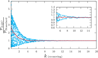
Power spectrum: As noted above, in bounces with kinetic energy domination on which we focus, the quantum state is known to remain sharply peaked on effective trajectories. Therefore, in numerical simulations a ‘mean field’ approximation was made by replacing by the mean values of these operators. For the background, several simulations were carried out with in , which, as we will see below, is the most interesting range. For perturbations, we used three different initial states in the class specified above. The power spectrum at the end of inflation was computed in each case for both scalar and tensor modes. Results are all very similar. FIG.1 shows how the LQC scalar power spectrum relates to the prediction of standard inflation for the case where , and the initial state is the ‘obvious’ or ‘standard’ 4th order adiabatic vacuum. We found that the plot is largely insensitive to choices of initial conditions within the class used in our simulations.
Recall, however, that the 7 year WMAP data wmap covers only a window in the co-moving space. Here the reference mode is the one that exits the Hubble radius at time when the Hubble parameter is given by . In FIG.1, numerical values of the co-moving were calculated using the scale factor convention , rather than . (The physical wave numbers are of course convention independent). In each simulation, we first locate the scale factor by setting , and then determine via . Since we have , values of and depend on the pre-inflationary background dynamics which turns out to be governed entirely by . Therefore, in FIG.1 the observationally relevant window depends on the value of , moving steadily to right as increases.
The plot has two interesting features. First, the LQG power spectrum is virtually indistinguishable from that of standard inflation if . This occurs when . Second, for smaller values of , the observational window admits modes for which the two power spectra are noticeably different. For concreteness, let us set . Then and these modes correspond to in the WMAP angular decomposition for which observational error bars are large. Therefore the LQG power spectrum is also viable but the predicted quantum state of perturbations at the onset of inflation is not the BD vacuum for .
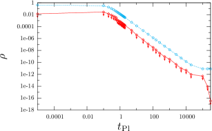
Self consistency: Whether the test field approximation continues to hold in the Planck regime is an intricate issue and had not been explored before. FIG.2 shows that we have obtained explicit self consistent solutions in which the renormalized energy density in perturbations remains low compared to the background all the way from the bounce to the onset of inflation. (Here, we have set , which corresponds to .) Furthermore, there is an analytical argument showing that every such admits a well-defined neighborhood (in the infinite dimensional space of the 4th order adiabatic ‘vacua’) with the same property. Thus, for , our truncated framework admits a rich set of self consistent solutions. Furthermore, in each of them has extremely small excitations over the BD vacuum at the onset of slow roll. These solutions provide viable extensions of the standard inflationary scenario all the way to the Planck scale.
What about the small but interesting window ? So far we only have upper bounds for the renormalized energy density in perturbations and these are far from being optimal. Therefore we do not yet have an explicit solution establishing the validity of the test field approximation in this window.
Summary and discussion: Using LQG ideas and techniques, we have extended the inflationary paradigm all the way to the deep Planck regime. At the big bounce, one can specify natural initial conditions for the quantum state that encodes the background homogeneous quantum geometry, as well as for that describes the quantum state of perturbations. There is a precise sense in which generic initial conditions for the background lead to a slow roll phase compatible with the 7 year WMAP data as3 . We have shown that there is a large set of initial data for such that: i) at the onset of slow roll, is extremely close to the BD vacuum, and, ii) the test field approximation behind the truncation strategy is self consistent. Each of these solutions provides a viable quantum gravity completion of the standard inflationary paradigm. However particle physics issues still remain.
In addition, there exists a narrow window, for which the quantum state at the onset of inflation has an appreciable number of ‘BD particles’ (but within the current observational limits). The physical origin of this effect can be explained in terms of the new scale defined by the universal value of the scalar curvature at the bounce. Excitations with are created in the Planck regime near the bounce. It turns out that if the number of e-foldings in between the bounce and is less than 15, then , whence some of these modes would be in the window accessible through CMB. corresponds to , precisely the regime in which the LQC power spectrum is different from the BD vacuum. Future measurements should be sensitive to such deviations halo-bias . If they are observed at the scale , the parameter space of initial conditions for would be tightly squeezed, making much more detailed predictions feasible. In this sense, the framework expands the reach of observational cosmology all the way to the deep Planck regime. This general argument also shows that the pre-inflationary dynamics has negligible effect for modes with because their physical wave lengths turn out to be smaller than the curvature scale throughout the evolution. This explains the very close agreement between the LQC and the standard power spectrum at high .
Finally, interesting and complementary investigations of LQG dynamics between the bounce and the onset of slow roll have appeared in the literature recently (see, especially, lqc ). The distinguishing features of our analysis are: i) It is based on the general truncation strategy that has proven to be successful in other problems; ii) It provides a systematic approach to quantum dynamics, made necessary by the fact that the classical evolution is not generated by a constraint on ; iii) The treatment of initial states has been stream-lined; and, most importantly, iv) While issues of regularization of the Hamiltonian operator , adiabatic renormalization of energy density, and consistency of the test field approximation were ignored so far, they have now been addressed using quantum field theory on quantum geometries. Details and subtleties which could not be included here will be discussed in two forthcoming articles.
Acknowledgments: This work is supported in part by the NSF grant PHY-1205388.
References
- (1) A. Borde, A. H. Guth and A. Vilenkin, Phys. Rev. Lett. 90, 151301 (2003).
- (2) I. Agullo and L. Parker, Phys. Rev. D83 063526 (2011); I. Agullo and S. Shandera, JCAP09, 007 (2012); J. Ganc and E. Komatsu, Phys. Rev. D86 023518 (2012).
- (3) For a review, see, e.g., A. Ashtekar and P. Singh, Class. Quant. Grav. 28, 213001 (2011).
- (4) See, e.g., K. Giesel and H. Sahlmann, 1203.2733; C. Rovelli, arXiv:1102.3660.
- (5) E. Komatsu et al, arXiv:hep-th/1001.4538
- (6) A. Ashtekar and D. Sloan, Gen. Rel. Grav. 43, 3619-3656 (2011); A. Corichi and A. Karami, Phys. Rev. D83,104006 (2011).
- (7) D. Langlois, Class. Quant. Grav. 11 389-407 (1994).
- (8) L. Parker and S. A. Fulling, Phys. Rev. D9 341 (1974).
- (9) J. Cortez, G. A. Mena Marugan, J. Olmedo, J. M. Velhinho, Phys. Rev. D83 025002 (2011).
- (10) T. Thiemann Introduction to modern canonical quantum general relativity (Cambridge University Press, Cambridge, 2005).
- (11) A. Ashtekar, T. Pawlowski and P. Singh (in preparation).
- (12) T. Pawlowski and A. Ashtekar, Phys. Rev. D85, 064001 (2012).
- (13) A. Ashtekar, W. Kaminski and J. Lewandowski, Phys. Rev. D79 064030 (2009).
- (14) T. Cailleteau, J. Mielczarek, A. Barrau and J. Grain, arXiv:1111.3535; M. Fernandez-Mendez, G. A. Mena Marugan, and J. Olmedo, arXiv:1205.1917. For LQG effects during inflation, see e.g., M. Bojowald, G. Calcagni and S. Tsujikawa, JCAP11, 046 (2011), and G. Calcagni, arXiv:1209.0473.