Line of Dirac monopoles embedded in a Bose-Einstein condensate

Abstract

The gauge field of a uniform line of magnetic monopoles is created using a single Laguerre-Gauss laser mode and a gradient in the physical magnetic field. We study the effect of these monopoles on a Bose condensed atomic gas, whose vortex structure transforms when more than six monopoles are trapped within the cloud. Finally, we study this transition with the collective modes.

A point source of magnetic flux, a magnetic monopole, has long been an important missing component of grand unified and superstring theories. Despite an exhaustive search for such monopoles Price75 ; Cabrera82 , no convincing evidence for the existence of a stable magnetic monopole has been forthcoming. Analogies to certain aspects of monopoles have been uncovered in physically tractable systems including spin ice Castelnovo08 , topological insulators Qi09 , the anomalous quantum Hall effect Fang03 , and superfluid ${}^{3}\text{He}$ Blaha76 . Nevertheless, the experimental realization of a true Dirac monopole remains an important target.

Over the past three years the cold atom gas has emerged as a promising new system in which to explore the motion of particles in magnetic fields Dalibard11 . Starting with a seminal experiment Lin08 ; Lin09 that imposed an effective uniform magnetic field on a Bose-Einstein condensate (BEC) of neutral atoms, the experimental protocol has been extended to realize spin-orbit coupling Lin11i , and effective electric fields Lin11ii . Following these successes, the spotlight has recently turned to generating the high magnetic fields required to study strongly correlated states such as the fractional quantum Hall effect Jaksch03 ; Mueller04 ; Gerbier10 ; Sorensen05 ; Alba11 ; Cooper11 ; Aidelsburger11 . However, cold atom gases also present a unique opportunity to study magnetic field configurations not realizable in the solid state, in particular a magnetic monopole Moody86 ; Ruseckas05 ; Pietila09i ; Pietila09ii . The experiments suggested to date demand either a laser setup of a superposition of Laguerre-Gauss modes along with Hermite-Gauss modes Moody86 ; Ruseckas05 ; Pietila09i , or three magnetic field modes Pietila09ii , which have not yet been realized in practice. Moreover, the configuration of a single monopole of fixed charge means that there is no tuning parameter that would allow the direct characterization of the state Pietila09i .

Here we propose a significantly simpler experimental protocol to embed a uniform line of monopoles into a BEC. Motivated by previous experiments Lin09 ; Lin11i ; Lin11ii that successfully realized effective gauge fields, our scheme adopts the same physical magnetic field gradient, and replaces the co-propagating laser plane waves with the first optical Laguerre-Gauss mode Wright00 ; Olson07 ; John11 . The system undergoes a transition with increasing monopole density, and we characterize the two phases by their collective modes spectra.

We first outline the experimental scheme to create the gauge field of a line of monopoles. Starting from the geometry in Fig. 1(a), we trap bosonic atoms that have three coupled internal levels (for example the $F=1$ manifold of ${}^{87}\text{Rb}$) labeled by $m_{\text{F}}$. We apply a small physical magnetic field $(B+B^{\prime}z)\hat{\mathbf{z}}$ where the magnetic field gradient $B^{\prime}$ could be generated by an anti-Helmholtz coil pair. The field introduces a linear Zeeman splitting so the atomic levels have energies $g\mu_{\text{B}}m_{\text{F}}B+m_{\text{F}}\delta$, where $\delta=g\mu_{\text{B}}B^{\prime}z$ is the detuning from the Raman resonance as shown in Fig. 1(c). Co-propagating Laguerre-Gauss laser beams induce the complex Rabi frequencies $\kappa_{\pm}=\kappa_{0}(\sqrt{2}\rho/\sqrt{\ell}w)^{\ell}\exp(\ell/2-\rho^{2}/w^{2}\pm\text{i}\ell\phi+\text{i}kz)$ Dalibard11 , with $\ell$ the beam winding number, $w$ the beam width, $\rho=\sqrt{x^{2}+y^{2}}$ the distance from the $z$-axis, $\phi$ the azimuthal angle, $\kappa_{0}$ the Rabi frequency at $\rho=w\sqrt{\ell/2}$, and $k$ the plane wave vector. The single-photon detuning $\Delta$ from the excited states manifold should be large versus the Rabi frequencies $\Delta\gg\kappa_{0}$ so that the excited states can be adiabatically eliminated and the Hamiltonian acts only on the ground state manifold.

(a) Geometric setup	(b) Magnetic field realized

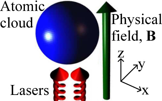
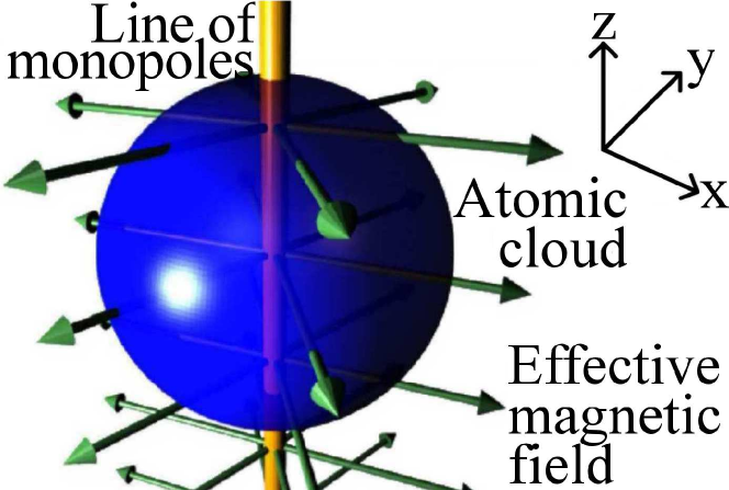
(c) Atomic level scheme	(d) Magnetic field error

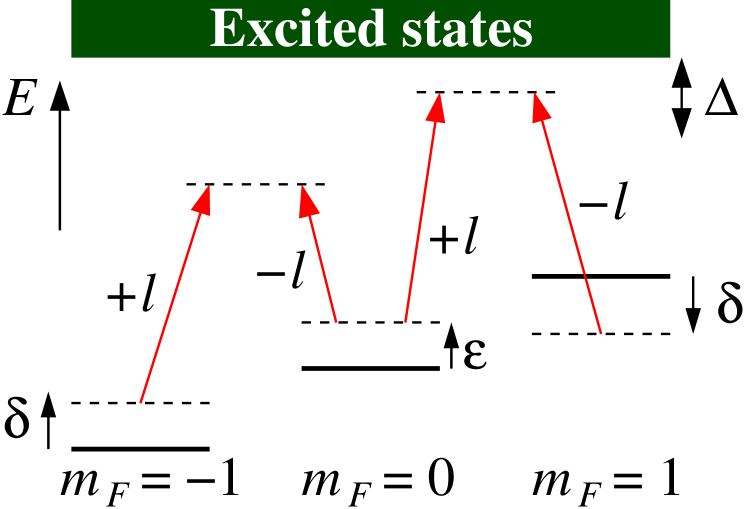
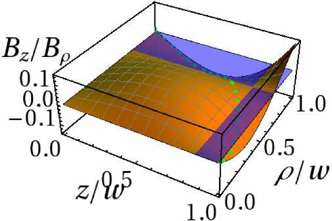
Figure 1: (Color online) (a) Geometry of the proposed scheme. Co-propagating laser beams with winding numbers $\pm\ell$ and the physical magnetic field $\mathbf{B}$ are aligned along $z$. (b) The gauge field realized, with the line of monopoles in orange, the effective magnetic field as green arrows, and the atomic cloud as the blue sphere. (c) The level diagram for the three electronic ground states displaced by the external physical magnetic field $\mathbf{B}$. The irradiating laser beams $+\ell$ and $-\ell$ induce resonant coupling. In practice $\Delta\gg\delta$. (d) The relative axial $B_{\text{z}}$ to radial magnetic field $B_{\rho}$. The dashed green line denotes the path of constant radius in the trap, and the blue sheet is $B_{\text{z}}/B_{\rho}=0$.

The Hamiltonian in the basis set $\{|m_{F}=-1\rangle,|m_{F}=0\rangle,|m_{F}=+1\rangle\}$ is $\hat{H}=(-\hbar^{2}\nabla^{2}/2m+\hat{V}-\mu)\mathsf{1}+\hat{U}$, with $m$ the atomic mass, the spin-independent trapping potential is $\hat{V}\!=\!m\omega^{2}(\rho^{2}\!+\!z^{2})/2$ with $\omega$ the trap curvature, and in the rotating wave approximation the coupling matrix is

$$\hat{U}=\frac{\hbar}{2}\left(\begin{array}[]{ccc}-2\delta&\kappa_{-}^{*}&0\\ \kappa_{-}&\epsilon\kappa_{0}&\kappa_{+}\\ 0&\kappa_{+}^{*}&2\delta\end{array}\right)\,,$$ (4)

with $\epsilon$ the quadratic Zeeman shift in units of $\kappa_{0}$. The three bands of the Hamiltonian are split by $\sim\kappa_{0}\gg\delta$. If the thermal energy and chemical potential $\mu$ Spielman09 are much lower than $\hbar\kappa_{0}$ Lin09 then only the ground state is occupied

$$|\chi\rangle\!=\!\text{e}^{2\text{i}\ell\phi}\cos^{2}\frac{\theta}{2}|-1\rangle\!-\!\frac{\sin\theta}{\sqrt{2}}|0\rangle\!+\!\text{e}^{-2\text{i}\ell\phi}\sin^{2}\frac{\theta}{2}|1\rangle\,,$$ (5)

with mixing angle $\tan{\theta}=|\kappa_{+}|/\sqrt{2}\delta$, and energy $-\hbar\sqrt{\delta^{2}+\kappa_{0}^{2}/2}$.

Following the prescription of Ref. Dalibard11 , we can calculate the gauge field as $\mathbf{A}=2\text{i}\hbar\langle\chi|\nabla\chi\rangle=\hbar\ell\cos\theta\hat{\bm{\phi}}/\rho$. The corresponding effective magnetic field is $\mathbf{B}=\nabla\times\mathbf{A}$ so

$$\!\!\!\left(\!\!\!\begin{array}[]{c}B_{\rho}\\ B_{\phi}\\ B_{\text{z}}\end{array}\!\!\!\right)\!\!=\!\frac{\hbar\ell\delta^{\prime}}{\kappa\rho[1\!+\!(\!\frac{z\delta^{\prime}}{\kappa_{0}}\!)^{\!2}]^{3/2}}\!\!\left(\begin{array}[]{c}1\\ 0\\ \!\!\!\frac{z}{\sqrt{\ell}w}\!\!\left[\!\alpha\!+\!\beta\frac{z^{2}}{w^{2}}\!\right]\!\!\left[2\!\left(\!\frac{\rho}{w}\!\right)^{2}\!\!-\!\ell\right]\!\!\end{array}\right)\!\!\,,$$ (12)

where $\alpha\!=\!\sqrt{2}\!+\!\epsilon\!+\!3\epsilon^{2}/10$ and $\beta\!=\!1/\sqrt{2}\!+\!\epsilon/2\!+\!17\epsilon^{2}/128$. The scalar potential defined by $W\!=\!\hbar^{2}[(\bm{\nabla}\theta)^{2}\!+\!\sin^{2}\theta(\bm{\nabla}\phi)^{2}]/8m$ is

$$W =\frac{\hbar^{2}}{2m}\frac{1}{\sqrt{1+\left(\frac{\delta^{\prime}z}{\kappa_{0}}\right)^{2}}}\Biggl{\{}\frac{1}{\sqrt{1+\left(\frac{\delta^{\prime}z}{\kappa_{0}}\right)^{2}}}\left(\frac{\ell}{\rho}\right)^{2}$$

$$+\left(\frac{\delta^{\prime}}{2\kappa_{0}}\right)^{2}\left[1+\left(\frac{z}{\rho}\right)^{2}\left(1-2\left(\frac{\rho}{w}\right)^{2}\right)^{2}\right]\Biggr{\}}\,.$$ (13)

After expressing the magnetic field gradient through $\delta=\delta^{\prime}z$, we expand these expressions in the $\kappa_{0}\gg\delta^{\prime}w$ limit, and about the radius $\rho_{\text{max}}=w\sqrt{\ell/2}$ of maximum laser beam intensity to yield the effective magnetic field

$$\left(\begin{array}[]{c}B_{\rho}\\ B_{\phi}\\ B_{\text{z}}\end{array}\right)\approx\frac{\sqrt{2}\hbar\ell\text{e}^{\ell}\delta^{\prime}}{\kappa_{0}\rho}\left(\begin{array}[]{c}1\\ 0\\ 0\end{array}\right)\,,$$ (20)

and in the same limit the scalar potential is $W=\hbar^{2}(\ell/\rho)^{2}/2m$. The effective magnetic field formed has the configuration shown in Fig. 1(b): it is directed radially and decays as $1/\rho$, so it represents the magnetic field emanating from a line of Dirac monopoles along $\hat{\mathbf{z}}$, with line density $2\sqrt{2}\ell\text{e}^{\ell}\delta^{\prime}/\kappa_{0}$. However, from Eqn. (12), $B_{\text{z}}=0$ only exactly at the radius $\rho_{\text{max}}=w\sqrt{\ell/2}$, but remains small away from it. To minimize $B_{\text{z}}$ over all radii we set $\epsilon=-2.8$, which yields the variation of $B_{\text{z}}/B_{\rho}$ shown in Fig. 1(d). Over the range of $\rho$ and $z$ within a trap (in Fig. 1(d) set so $\rho^{2}+z^{2}<w^{2}$) we find that $|B_{\text{z}}/B_{\rho}|<0.1$ and so the effective field closely approximates that of a line of monopoles. We also note that the anti-Helmholtz coil pair necessarily generates a radial physical magnetic field gradient as well as the $B^{\prime}$ along the $z$-axis. This generates a $B_{\text{z}}$ component that could also be removed by the quadratic Zeeman shift. In both cases as $\mathbf{A}$ is continuous away from $\rho=0$ flux is conserved and the only monopoles lie along the $z$-axis. The $B_{\text{z}}$ component of the effective magnetic field is then a small field component corresponding to a changing line density of monopoles. This will be further tested in Fig. 2 by comparing the BEC ground state for both gauge fields.

To probe the experimental prospects of the proposed configuration we first check the maximum achievable monopole density. For $\ell=1$, using the realistic Lin09 values $\delta^{\prime}=4.5E_{\text{r}}/\mu\text{m}$ and $\kappa_{0}=16E_{\text{r}}$, with $E_{\text{r}}$ the recoil energy, a cloud of diameter $d=80\mu\text{m}$ contains $N=2\sqrt{2}\text{e}\delta^{\prime}d/\kappa_{0}\approx 80$ monopoles. We adopt the natural definition of monopole charge density so that the flux quantum $\Phi_{0}$ emanating from a single charge winds the phase of the BEC by a factor of $2\pi$.

Having formed the effective gauge field of a line of monopoles, we now develop the formalism to study its influence on a BEC. To seek and study the ground state we discretize Pietila09i ; Pietila09ii the Hamiltonian onto a lattice of spacing $a$. The derivative at a lattice site $\mathbf{R}=\{x,y,z\}$ along a single link $\mathbf{r}$ is transformed to $[D_{\mathbf{r}}\psi(\mathbf{R})]^{\dagger}[D_{\mathbf{r}}\psi(\mathbf{R})]\to(\psi_{\mathbf{R}+\mathbf{r}}-U_{\mathbf{R},\mathbf{r}}\psi_{\mathbf{R}})^{\dagger}(\psi_{\mathbf{R}+\mathbf{r}}-U_{\mathbf{R},\mathbf{r}}\psi_{\mathbf{R}})/a^{2}\equiv C_{\mathbf{R},\mathbf{r}}$, where the hopping matrix is $U_{\mathbf{R},\mathbf{r}}=\exp(\text{i}\mathbf{A}(\mathbf{R})\cdot\mathbf{r}/\hbar)$, and $\psi_{\mathbf{R}}$ is the condensate order parameter at $\mathbf{R}$. With this in place the mean-field energy is

$$E\!=\!\frac{\hbar^{2}}{2m}\!\sum_{\mathbf{R},\mathbf{r}}\!C_{\mathbf{R},\mathbf{r}}\!+\!\sum_{\mathbf{R}}\!\left[(V_{\mathbf{R}}\!+\!W_{\mathbf{R}}\!-\!\mu)|\psi_{\mathbf{R}}|^{2}\!+\!\frac{c}{2}|\psi_{\mathbf{R}}|^{4}\right]\!\,,$$

with external potential $V_{\mathbf{R}}\!=\!m\omega^{2}(x^{2}\!+\!y^{2}\!+\!z^{2})/2$, and a chemical potential $\mu$ to fix the number of particles. We minimize the free energy variationally with respect to $\psi_{\mathbf{R}}^{*}$ to yield the discrete Gross-Pitaevskii (GP) equation

$$\mu\psi_{\mathbf{R}}= -\frac{\hbar^{2}}{2ma^{2}}\sum_{\mathbf{r}}\left(U_{\mathbf{R},\mathbf{r}}^{*}\psi_{\mathbf{R}+\mathbf{r}}-2\psi_{\mathbf{R}}+U_{\mathbf{R}-\mathbf{r},\mathbf{r}}\psi_{\mathbf{R}-\mathbf{r}}\right)$$

$$+\left(V_{\mathbf{R}}+W_{\mathbf{R}}+c|\psi_{\mathbf{R}}|^{2}\right)\psi_{\mathbf{R}}\,.$$ (21)

To calculate the ground state we solve the GP equations iteratively using the over-relaxation scheme on a grid of $200\times 200\times 200$ sites with periodic boundary conditions.

With a tool to determine the ground state wave function in place, to calculate the collective mode spectrum we adopt the linear-response theory Edwards96 that was successfully used to study the excitation frequencies of a uniform BEC in a vortex state Dodd97 . We first substitute the general form for the solution of the Gross-Pitaevskii equation

$$\Psi_{\mathbf{R},t}=\text{e}^{\text{i}\mu t/\hbar}\left[\psi_{\mathbf{R}}+u_{\lambda,\mathbf{R}}\text{e}^{-\text{i}\Omega_{\lambda}t}+v_{\lambda,\mathbf{R}}^{*}\text{e}^{\text{i}\Omega_{\lambda}t}\right]\,,$$ (22)

into the Hamiltonian. Here $\psi_{\mathbf{R}}$ is the ground state wave function and $\lambda$ is the index of the eigenvalue $\Omega_{\lambda}$ with eigenfunctions $u_{\lambda,\mathbf{R}}$ and $v_{\lambda,\mathbf{R}}$. This recovers the time-independent Gross-Pitaevskii equation for $\psi_{\mathbf{R}}$ along with the linear-response Bogoliubov equations

$$\left(\begin{array}[]{cc}\mathcal{L}_{\mathbf{R}}&-\frac{c}{2}|\psi_{\mathbf{R}}|^{2}\\ \frac{c}{2}|\psi_{\mathbf{R}}|^{2}&-\mathcal{L}_{\mathbf{R}}\end{array}\right)\left(\begin{array}[]{c}u_{\lambda,\mathbf{R}}\\ v_{\lambda,\mathbf{R}}\end{array}\right)=\hbar\Omega_{\lambda}\left(\begin{array}[]{c}u_{\lambda,\mathbf{R}}\\ v_{\lambda,\mathbf{R}}\end{array}\right)\,,$$ (29)

with $\mathcal{L}_{\mathbf{R}}=-\hbar^{2}\sum_{\mathbf{r}}(U^{*}_{\mathbf{R}-\mathbf{r},\mathbf{r}}-2+U_{\mathbf{R},\mathbf{r}})/2ma^{2}+V_{\mathbf{R}}+W_{\mathbf{R}}-\mu+c|\psi_{\mathbf{R}}|^{2}$. Using the condensate order parameter for the ground state, we use the Arnoldi method to solve the Bogoliubov equations to find the lowest eigenstates and eigenmodes that are the collective modes.

	(a) $N=4$, realized		(b) $N=12$, realized

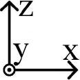
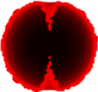
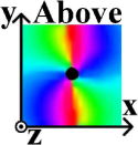
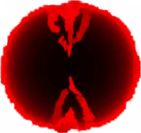
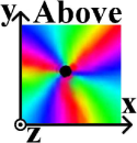
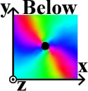
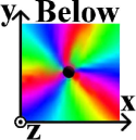
(c) $N=55$	(d) $N=4$	(e) $N=12$	(f) $N=55$
realized	idealized	idealized	idealized

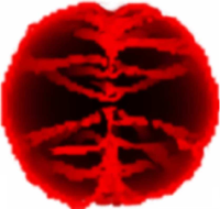
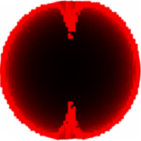
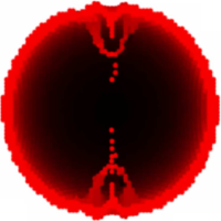
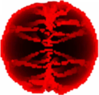
Figure 2: (Color online) The particle density isosurfaces of BECs containing (a) $N=4$, (b) $N=12$, (c) $N=55$ monopoles for the gauge field of the proposed setup. The isosurfaces for the artificial situation of a perfect line of (d) $N=4$, (e) $N=12$, and (f) $N=55$ monopoles. The brightness denotes the depth of the site on the $y$-axis. The right-hand plots of (a,b) view the condensate along the $z$-axis, and use the hue to display the condensate phase.

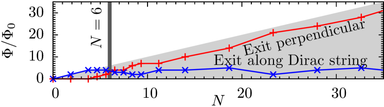
Figure 3: (Color online) Flux $\Phi$ exiting the cloud as a function of the number of embedded monopoles $N$. The red line $(+)$ shows the flux exiting radially, the blue line $(\times)$ the flux exiting along the Dirac string. The grey shading denotes the region where the escaping flux is necessarily less than the monopolar charge contained. The vertical black line shows the theoretically predicted crossover when flux first exits away from the string.

With the physical setup and numerical procedure in place, we now study the ground state configuration of our trapped BEC embedded with a line of monopoles. We first examine the phase behavior of the ground state with increasing monopole density. Second, to fully characterize the state, we calculate their collective mode spectrum. We study $100\mathord{,}000$ atoms in a spherical trap with $\omega=0.1$ and interaction strength $c=0.05$ in atomic units $\hbar=m=1$. The Laguerre-Gauss beams have winding number $\ell=1$ and beam width $w=40a$, and vary the detuning gradient $\delta^{\prime}/\kappa_{0}$ to control the monopolar charge density, which within a characteristic length $w$ of the center is $4\sqrt{2}\text{e}\delta^{\prime}w/\kappa_{0}$. We use the realistic gauge field $\mathbf{A}=2\hbar\cos\theta\hat{\bm{\phi}}/\rho$.

With no embedded monopoles the BEC is spherically symmetric in the trap. In Fig. 2(a) we examine the density isosurfaces for a cloud that encloses $N=4$ monopolar charges. The density falls along the $z$-axis and the phase of the condensate order parameter winds by $4\pi$ around the $z$-axis showing that the flux escapes symmetrically through the top and bottom of the cloud forming vortices. On increasing the number of trapped monopoles to $N=12$, in Fig. 2(b) now three flux quanta pass through the top of the cloud, and a further three through induced vortices directed away from the axis in the upper hemisphere, with the situation repeated in the lower hemisphere. The stepwise change where flux starts to escape away from the $z$-axis occurs at $N\approx 6$. The cylindrical symmetry of the cloud is broken by the random site updates on the computational lattice. When a large number of monopoles $N=55$ are trapped by the cloud in Fig. 2(c) we observe that the vast majority of the flux escapes through the side of the cloud broadly symmetrically. Finally, we compare the predictions for the gauge field realized by the proposed laser setup, $\mathbf{A}=2\hbar\cos\theta\hat{\bm{\phi}}/\rho$ (Fig. 2(a,b,c)), with an idealized $\mathbf{A}=4\text{e}\hbar\delta\hat{\bm{\phi}}/\kappa_{0}\rho$ of the artificial situation of the magnetic field of a perfect line of monopoles (Fig. 2(d,e,f)). The distribution of the vortices formed by the exiting flux are broadly similar. Therefore the gauge field realized by the laser setup accurately models that of an ideal line of monopoles. We also checked the stability of the results while changing the random number seed of the lattice updates, boundary conditions between periodic and hard wall, the orientation of the line of monopoles relative to the lattice, and lattice size.

Having studied clouds containing different monopolar charges, we now summarize their behavior in Fig. 3. In particular we focus on the route of the escaping flux, which is along the $z$-axis for $N\lesssim 5$ and penetrates through the side walls of the cloud for $N\gtrsim 8$. When $N\gtrsim 8$, the flux still exits along the $z$-axis, but remains fewer than a total of $\sim 6$ flux quanta. To understand why there is a transition in behavior at $5\lesssim N\lesssim 8$ we can compare the energy cost of flux exiting the cloud through the two different routes. The energy of a vortex per unit length is $C\gamma^{2}$ Bruun01 where $\gamma$ is the number of circulation quanta of the vortex and $C$ a constant defined in Bruun01 . For a system of radius $R$, length $L$, and monopole line density $\eta$, the energy of all the flux escaping along the $z$-axis is $C\eta^{2}L^{3}/12$, whereas if the flux exits radially the total energy is $C\eta LR$. Therefore the flux exits radially when $12R>\eta L^{2}$. Here the cost of multiple flux quanta exiting along the same vortex line out of the top or bottom of the cloud is outweighed by the energy cost of flux exiting through longer vortex lines out of the cloud sides. For a spherically symmetric trap where $L=2R$ and $N=\eta L$, the flux exits radially when $N\geq 6$. This can be readily seen in Fig. 3 where flux exiting radially rises rapidly when more than six flux quanta are enclosed by the cloud. Here, as in previous studies of rotation-induced vortices in BECs, the vortices will be too small to image directly. However, if the cloud is ballistically expanded the vortices are magnified and could be imaged Dalibard00 ; Shaeer01 ; Engels02 ; Coddington03 .

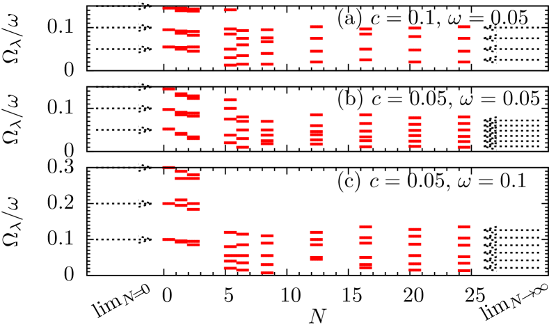
Figure 4: (Color online) The collective mode frequencies renormalized by the trapping potential $\Omega_{\lambda}/\omega$ as a function of number of embedded monopoles $N$ for different interaction strengths and trapping potentials. The dashed arrows highlight the expected modes in the $N=0$ and $N\to\infty$ limits.

On top of direct imaging, a second experimental tool to characterize the BEC with embedded monopoles is the collective mode spectrum. This was previously used to analyze both the uniform and rotation-induced vortices in BECs Jin96 ; Edwards96 ; Stringari96 ; Dodd97 ; Coddington03 . Collective modes can be excited by a red-detuned optical dipole potential that draws atoms into the center of the condensate Coddington03 .

To study the collective mode spectrum of the cloud we take the ground state wavefunction and diagonalize the linear response Bogoliubov equations. In Fig. 4 we show the lowest mode frequencies for a series of clouds with differing numbers $N$ of embedded monopoles. We first compare the observed spectra at $N=0$ to that of a vortex-free BEC in a spherical trap whose collective modes in the weakly interacting limit are simply the single-particle modes in the parabolic trapping potential, so $\Omega_{\lambda}=\lambda\omega$ with $\lambda\in\mathbb{Z}^{+}$. These frequencies are in good agreement with the calculated modes, and double in energy on doubling $\omega$ from (b) to (c), but barely change on reducing the interaction strength $c$ from (a) to (b). On increasing $N\lesssim 6$ the flux quanta initially escape along the $z$-axis, breaking the spherical symmetry, and splitting the degenerate modes. With a large number of embedded monopoles $N\to\infty$ the surface of the cloud resembles a two-dimensional BEC penetrated by a vortex lattice (see for example Fig. 2(c)). The modes of such a sheet are $\Omega=h[nc(n_{\text{x}}^{2}+n_{\text{y}}^{2}+n_{\text{z}}^{2})/m]^{1/2}$ Sonin87 , with $\{n_{\text{x}},n_{\text{y}},n_{\text{z}}\}\in\mathbb{Z}$, $n$ the density, and $L$ the sheet size, here the circumference of the cloud. These modes were verified by their frequencies halving on reducing the interaction strength from (a) to (b). This provides an intuitive picture of the low energy collective modes in the $N\to\infty$ limit where the surface modes dominate. With these signatures the collective modes could help diagnose the behavior of the BEC embedded with monopoles.

In this paper we have constructed a gauge field of a line of magnetic monopoles embedded in a BEC. The BEC underwent a transition from channeling the flux along the Dirac string to the flux escaping out of the cloud walls. Finally, we characterized this transition through the collective modes spectrum. However, there are opportunities to explore monopolar gauge fields in two other systems. The first is to study the single atom bound states in a non-interacting gas. These feel the same effective magnetic field as the condensate atoms, and could be characterized by exciting transitions between different states. The second possibility is to generalize our single spin species BEC up to a two-component BEC by exploiting a multi-level system with doubly degenerate dark states and study the emergence of topological states Pietila09i .

Acknowledgments: The author acknowledges the financial support of Gonville & Caius College.

References

- (1) B. Cabrera, Phys. Rev. Lett., 48, 1378 (1982).
- (2) P.B. Price, E.K. Shirk, W.Z. Osborne, and L.S. Pinsky, Phys. Rev. Lett., 35, 487 (1975).
- (3) C. Castelnovo, R. Moessner, and S.L. Sondhi, Nature 451, 42 (2008).
- (4) X.-L. Qi et al., Science 323, 1184 (2009).
- (5) Z. Fang et al., Science 302, 92 (2003).
- (6) S. Blaha, Phys. Rev. Lett., 36, 874 (1976).
- (7) J. Dalibard, F. Gerbier, G. Juzeliūnas, and P. Öhberg, Rev. Mod. Phys, 83, 1523 (2011).
- (8) Y.-J. Lin, R.L. Compton, K. Jiménez-García, J.V. Porto, and I.B. Spielman, Nature 462, 628 (2009).
- (9) Y.-J. Lin, R.L. Compton, A.R. Perry, W.D. Phillips, J.V. Porto, and I.B. Spielman, Phys. Rev. Lett. 102, 130401 (2009).
- (10) Y.-J. Lin, K. Jiménez-García, and I.B. Spielman, Nature 471, 83 (2011).
- (11) Y.-J. Lin, R.L. Compton, K. Jiménez-García, W.D. Phillips, J.V. Porto, and I.B. Spielman, Nature Physics 7, 531 (2011).
- (12) N.R. Cooper, Phys. Rev. Lett., 106, 175301 (2011).
- (13) M. Aidelsburger, M. Atala, S. Nascimbène, S. Trotzky, Y.-A. Chen, and I. Bloch, Phys. Rev. Lett. 107, 255301 (2011).
- (14) D. Jaksch and P. Zoller, New J. Phys. 5, 56 (2003).
- (15) E.J. Mueller, Phys. Rev. A 70, 041603 (2004).
- (16) F. Gerbier and J. Dalibard, New J. Phys. 12, 033007 (2010).
- (17) A.S. Sørensen, E. Demler, and M.D. Lukin, Phys. Rev. Lett. 94, 086803 (2005).
- (18) E. Alba, X. Fernandez-Gonzalvo, J. Mur-Petit, J.K. Pachos, and J.J. Garcia-Ripoll, Phys. Rev. Lett. 107, 235301 (2011).
- (19) J. Moody, A. Shapere, and F. Wilczek, Geometric Phases in Physics (1989).
- (20) J. Ruseckas, G. Juzeliūnas, P. Öhberg, and M. Fleischhauer, Phys. Rev. Lett., 95, 010404 (2005).
- (21) V. Pietilä, and M. Möttönen, Phys. Rev. Lett., 102, 080403 (2009).
- (22) V. Pietilä, and M. Möttönen, Phys. Rev. Lett., 103, 030401 (2009).
- (23) E.M. Wright, J. Arlt, and K. Dholakia, Phys. Rev. A, 63, 013608 (2000).
- (24) S.E. Olson, M.L. Terraciano, M. Bashkansky, and F.K. Fatemi, Phys. Rev. A, 76, 061404(R) (2007).
- (25) S.T. John, Z. Hadzibabic, and N.R. Cooper, Phys. Rev. A, 83, 023610 (2011).
- (26) I.B. Spielman, Phys. Rev. A, 79, 063613 (2009).
- (27) M. Edwards, P.A. Ruprecht, K. Burnett, R.J. Dodd, and C.W. Clark, Phys. Rev. Lett., 77, 1671 (1996).
- (28) R.J. Dodd, K. Burnett, M. Edwards, and C.W. Clark, Phys. Rev. A, 56, 587 (1997).
- (29) I. Coddington, P. Engels, V. Schweikhard, and E.A. Cornell, Phys. Rev. Lett., 91, 100402 (2003).
- (30) K.W. Madison, F. Chevy, W. Wohlleben, and J. Dalibard, Phys. Rev. Lett. 84, 806 (2000).
- (31) P. Engels, I. Coddington, P.C. Haljan, V. Schweikhard, and E.A. Cornell, Phys. Rev. Lett., 90, 170405 (2003).
- (32) J.R. Abo-Shaeer, C. Raman, J.M. Vogels, and W. Ketterle, Science 292, 476 (2001).
- (33) S. Stringari, Phys. Rev. Lett., 77, 2360 (1996).
- (34) D.S. Jin, J.R. Ensher, M.R. Matthews, C.E. Wieman, and E.A. Cornell, Phys. Rev. Lett., 77, 420 (1996).
- (35) E.B. Sonin, Rev. Mod. Phys., 59, 87 (1987).
- (36) G.M. Bruun, and L. Viverit, Phys. Rev. A 64, 063606 (2001).