The regular conducting fluid model for relativistic thermodynamics

Abstract

The “regular” model presented here can be considered to be the most natural solution to the problem of constructing the simplest possible relativistic analogue of the category of classical Fourier–Euler thermally conducting fluid models as characterised by a pair of equations of state for just two dependent variables (an equilibrium density and a conducting scalar). The historically established but causally unsatisfactory solution to this problem due to Eckart is shown to be based on an ansatz that is interpretable as postulating a most unnatural relation between the (particle and entropy) velocities and their associated momenta, which accounts for the well known bad behaviour of that model which has recently been shown to have very pathological mixed-elliptic-hyperbolic comportments. The newer (and more elegant) solution of Landau and Lifshitz has a more mathematically respectable parabolic-hyperbolic comportment, but is still compatible with a well posed initial value problem only in such a restricted limit-case such as that of linearised perturbations of a static background. For mathematically acceptable behaviour under more general circumstances, and a fortiori for the physically motivated requirement of subluminal signal propagation, only strictly hyperbolic behaviour is acceptable. Attention is drawn here to the availability of a more modern “regular” solution which, unlike those of Eckart and of Landau and Lifshitz, is fully satisfactory as far as all these requirements are concerned. This “regular” category of relativistic conducting fluid models arises naturally within a recently developed variational approach, in which the traditionally important stress–momentum-energy density tensor is relegated to a secondary role, while the relevant covariant 4-momentum co-vectors are instead brought to the fore in such a way as to suggest a simplifying ansatz that is obviously more natural than those of Eckart and of Landau and Lifshitz, and automatically takes care of the causality problem.

1 Introduction: the three current theories

Until recently, there was no universally accepted solution to the problem of constructing a physically satisfactory relativistic analogue of the standard (general purpose) Euler–Fourier theory of a thermally conducting fluid, even in its simplest version as an eight component “two by two” category of hydrodynamic models in which the eight independent field components may be considered to be the space-time coordinate components of a particle number current vector, $n^{\nu}$, and an entropy vector, $s^{\nu}$ say, where a specific model within the category is fully characterised by just two equations of state involving just two independent variables, the latter being conveniently considered as an entropy density, $s$ say, and a conserved particle density, $n$ say, (as defined with respect to a frame whose appropriate choice will be seen to be crucial for the good behaviour of the theory) with the dependent variables taken as a mass-energy density function, $\rho$ say, and a thermal conductivity scalar $\kappa$ say, as given by a pair of equation of state functions, $\rho(s,\,n)$ and $\kappa(s,\,n)$, whose form may be considered to be obtainable completely from (experimental or theoretical) knowledge only of the thermal equilibrium limit.

The earliest and most widely known proposal leading to a category of this type was provided by the theory of Eckart [1], which has often been accorded [2] the status of “standard textbook solution” to the problem, despite the fact that it has been long recognised [3] as being unsatisfactory from the point of view of compatibility with relativistic causality. It was long thought to share this with its non-relativistic (Euler-Fourier) prototype the property of being mixed parabolic-hyperbolic type, rather than strictly hyperbolic that one would desire not only on physical grounds as a prerequisite for relativistic causality, but also on mathematical grounds as a prerequisite for the existence of Cauchy hyper-surfaces admitting a well-posed initial value problem in circumstances more general than the strictly static case. However in fact, as was already indicated by the work of Glaviano and Raymond [4], and as has been made particularly clear by the more recent stability analysis of Hiscock and Lindblom [5], the Eckart theory is far worse in so far as it has the mathematically and physically pathological property of being of mixed elliptic-hyperbolic type. As such it is incompatible with stable evolution from freely specified initial data on a space-like hyper-surface, even in the case of small perturbations on a static background, (so that any attempt to use it for numerical computations could be expected to lead to disaster).

Another such “two by two” category is provided by the newer theory of Landau and Lifshitz [6], which has long been unduely neglected, apparently because it was reputed to be “essentially equivalent” (modulo “unimportant” correction terms of quadratic or higher order in deviations from thermal equilibrium) to a mere reformulation of the Eckart theory in a new reference system. In fact however the work of Hiscock and Lindblom has it made clear that the Landau–Lifshitz theory is in fact a distinct improvement on its predecessor in so far as it actually does have the marginally hyperbolic character that was wrongly believed to characterise the Eckart model, meaning, to be more explicit, that it is of mixed parabolic-hyperbolic type. It is thus at least mathematically well behaved in the restricted context of linearised perturbations on a strictly static background, on which it admits the posing of well behaved initial value problems.

Despite this substantial advantage of mathematical respectability in this limited sense (in view of which the correction terms by which it differs from the Eckart model can hardly be dismissed as entirely unimportant) the Landau–Lifshitz theory still has the seriously unsatisfactory feature of being incompatible with the strict hyperbolicity property needed not only for the physical desideratum of subliminal propagation in accordance with the usual relativistic causality requirement, but also for the mathematical requirement of the existence of well behaved Cauchy surfaces (even in the stationary but non-static case for which parabolic type characteristic elements orthogonal to the flow would not be integrable). The purport of this present communication is to convey the message that the Landau–Lifshitz category should itself now be considered as having been made obsolete by the more recent construction [7] of a third such “two by two” category that is satisfactorily compatible with physical as well as mathematical causality requirements, and whose use may therefore safely be recommended for a wide range of astrophysical applications. This “regular” category arises as the natural outcome of the a recently developed variational approach [8] in which the 4-momentum co-vectors replace the more traditional stress-momentum-energy tensor as fundamental entities in the formulation of the theory.

Although the time is long overdue for the Eckart theory to be demoted from standard textbook status that has been perpetuated by Weinberg [2, 9], and others, and to be relegated to to the rank of historical curiosity, the Landau–Lifshitz theory remains nevertheless of some genuine mathematical interest as a distinguished limit case that might even be practically utilisable as an approximation in very special circumstances. However if one wants a simple trouble-free model for general purpose use, it is the “regular” theory that should be used.

It is to be mentioned, of course, that while it is entirely suitable of replacing the Eckart model in textbooks for the role of a general purpose “off the peg” conductivity theory, neither the “regular” nor any other such simple “two by two” category of models involving only eight independent component variables can compete with the much more elaborate categories involving fourteen independent variables that have been developed by the work of Müller [10], Israel [11] and Stewart [12], the extra six components corresponding to viscous degrees of freedom that are not taken into account in the simpler models discussed here (and that are in fact negligible in a wide range of relevant application to problems such as thermal diffusion in stellar interiors). While such much more complicated fourteen components models have the advantage of being able to fit detailed applications with comparitivity high precision if enough is known of numerous relevant parameters and equation of state functions, they have the corresponding disadvantage of being unnecessary unweildy and uneconomical for many other applications in which such complicated and detailed information is either undesirable or unavailable.

2 The formally identical differential equations of the three theories in their standardised from

Although they were originally set up using different notation schemes adapted to the different motivational considerations by which the three (Eckart, Landau–Lifshitz, and “regular”) theories referred to above were first obtained (this is the reason why it took so long before the difference between the two former was recognised), it is possible to clarify the relationship between them by converting them to a “standardised” form in which the necessary differential equations in all the three cases are formally identical, only the algebraic relations between the quantities involved being different from one category to another. In all three cases the first of the primary equations of state functions, $\rho(n,\,s)$ and $\kappa(n,\,s)$, may be used to derive secondary equation of state functions for variables $\mu$, $\Theta$, $P$, respectively interpretable as chemical potential, temperature and pressure in accordance with formulae of form that is familiar from the standard thermal equilibrium theory, namely

$$\mu=\frac{\partial\rho}{\partial n}\;\;,\qquad\Theta=\frac{\partial\rho}{\partial s}\;\;,\qquad P=n\mu+s\Theta-\rho\;\;.$$ (1)

In all three cases it is possible to obtain a basic conductivity equation in the form that has been made widely familiar by the many advocates of the Eckart theory, namely

$$Q^{\mu}=-\kappa\Big{(}\gamma^{\mu\nu}\nabla_{\nu}\Theta+\dot{u}^{\mu}\Theta\Big{)}\;\;,$$ (2)

the remaining differential equations being the entropy creation formula

$$\nabla_{\nu}s^{\nu}=\frac{Q^{\mu}Q_{\mu}}{\kappa\Theta^{2}}\;\;,$$ (3)

the usual particle conservation

$$\nabla_{\nu}n^{\nu}=0\;\;,$$ (4)

and the stress-momentum-energy (pseudo) conservation law,

$$\nabla_{\nu}T^{\nu}_{\phantom{\nu}\mu}=0\;\;,$$ (5)

where the projected space-metric tensor, $\gamma^{\mu\nu}$, and the acceleration vector, $\dot{u}^{\mu}$, are defined in terms of the ordinary (pseudo-Riemanian) space-time metric tensor, $g_{\mu\nu}$, and of a certain preferred time-like unit vector, $u^{\mu}$, in the usual manner, so that one has

$$\gamma^{\mu\nu}=u^{\mu}u^{\nu}+g^{\mu\nu}\;\;,\quad\dot{u}^{\mu}=u^{\nu}\nabla_{\nu}u^{\mu}\;\;,\quad u^{\nu}u_{\nu}=-1\;\;.$$ (6)

In all three cases the heat flux vector $Q^{\mu}$ is defined in terms of an appropriate heat transport vector $v^{\mu}$ by an expression of the form

$$Q^{\mu}=\Theta sv^{\mu}\;\;,\quad v^{\nu}u_{\nu}=0\;\;.$$ (7)

Although it was not done in the original derivation of the two older theories, it is also possible in all three cases (and greatly helps to clarify the comparison between them) to express the stress-momentum-energy density tensor in the “canonical” form

$$T^{\nu}_{\phantom{\nu}\mu}=n^{\nu}\chi_{\mu}+s^{\nu}\Theta_{\mu}+Pg^{\nu}_{\phantom{\nu}\mu}\;\;,$$ (8)

in terms of co-vectors, $\chi_{\mu}$ and $\Theta_{\mu}$, respectively interpretable as the “chemical” 4-momentum (per conserved particle) and the “thermal” 4-momentum (per unit entropy).

3 The essential distinct algebraic structural relations or the three models

Despite the apparent identity of the foregoing formal equations of motion of all three theories, they nevertheless differ radically in their dynamical behaviour, as a result of essential differences between the remaining purely algebraic structural relations that are needed to complete the specification of the theories. The foregoing description can be seen to involve a total of three subsets of each of eight distinct component variables, so it thus remains a prescription determining two of these subsets in terms of the third, since ultimately there should only be eight truly independent variables in the theory. In the original Eckart theory and in the new “regular” theory the most natural choice for the eight independent variables is the set of components of the two basic current 4-vectors, $n^{\mu}$ and $s^{\mu}$, whereas in the Landau–Lifshitz theory it is a little more convenient to take the eight independent variables to be the distinct subset consisting of the two scalars $n$ and $s$, together with the six components of the unit vector $u^{\mu}$ and the orthogonal vector $v^{\mu}$; the third set of the eight variables that needs to be determined (and which would themselves be the fundamental ones in a Clebsch type Legendre transformed reformulation of the perfectly conducting limit) are the components of the 4-momentum co-vectors, $\chi_{\mu}$ and $\Theta_{\mu}$.

Eight of the sixteen required algebraic component relationships can conveniently be expressed in a form that (as was the case for the differential relations of the preceding section) is the same for all the three cases. To start with the transport velocity vector is always expressible in form of the (“bulk” or “baryonic” flow) unit vector, $b^{\mu}$ say, along the direction of the conserved particle flux, $n^{\nu}$, and of the (“caloric” flow) unit vector, $c^{\mu}$ say, along the direction of entropy flux, $s^{\mu}$, in the form

$$v^{\mu}=\frac{b^{\mu}}{b^{\nu}u_{\nu}}-\frac{c^{\mu}}{c^{\nu}u_{\nu}}\;\;,$$ (9)

where explicitly

$$b^{\mu}=\frac{n^{\nu}}{\sqrt{-n^{\nu}n_{\nu}}}\;\;,\qquad c^{\mu}=\frac{s^{\nu}}{\sqrt{-s^{\nu}s_{\nu}}}\;\;.$$ (10)

It is also possible in all three cases to express the entropy scalar, $s$, and the effective thermal 4-momentum co-vector, $\Theta_{\mu}$, in the form

$$s=-s^{\nu}u_{\nu}$$ (11)

and

$$\Theta_{\mu}=\Theta\,u_{\mu}\;\;.$$ (12)

To complete the specification of the theories, however, one still needs eight more algebraic component relations, namely, an analogue of (9) to fix the (three independent) components of $u^{\mu}$, an analogue of (11) to fix the number density scalar, $n$, and an analogue of (12) to fix the particle 4-momentum, $\chi_{\mu}$, and it is at this stage that the distinction between the theories become apparent. Indeed the historical deviations of both the Eckart and the Landau–Lifshitz theories were based on distinct choices of preferred time-like unit vector at the outset. The Eckart choice, corresponding to the “conserved particle rest-frame”, is expressible in the present notation scheme by simply as

$$u^{\mu}=b^{\mu}\;\;.$$ (13a)

The Landau–Lifshitz choice, corresponding to the time-like eigenvalue of the stress-momentum-energy density tensor, is expressible in the present notation scheme as

$$u^{\mu}=\frac{\mu n^{\mu}+\Theta s^{\mu}}{\mu n+\Theta s}\;\;.$$ (13b)

My original deviation of the “regular” model used a more covariant approach, avoiding excessive reliance on any single “preferred rest-frame” but when this newer theory is translated into the present notation scheme it turns out that it requires that the preferred unit vector should correspond to the “thermal rest-frame” as determined by the entropy current, i.e. one needs to take

$$u^{\mu}=c^{\mu}\;\;.$$ (13c)

Let us now move on to consider the particle density scalar, $n$. In the Eckart theory it is defined with respect to the conserved particles’ own rest-frame which in this case corresponds to the preferred reference system, i.e. one has

$$n=-n^{\nu}b_{\nu}=-n^{\nu}u_{\nu}\;\;.$$ (14a)

In the Landau–Lifshitz theory $$n$$ is again defined with respect to a preferred reference system, but it no longer coincides with the particles’ own rest-frame, so one just has

$$n=-n^{\nu}u_{\nu}\;\;.$$ (14b)

On the other hand in the “regular” theory it is the particles’ own rest-frame not the preferred reference system that must be chosen, i.e. one needs to take

$$n=-n^{\nu}b_{\nu}\;\;.$$ (14c)

Up to the present stage in this presentation there is nothing that makes it particularly obvious why only the last choice should be fully satisfactory, why the second is marginally admissible, and why the first is entirely unacceptable. However the situation becomes much clearer when we have specified the relation for the particle 4-momentum, $\chi_{\mu}$ (a concept which of course was not explicitly mentioned at all in the original derivations of the two earlier theories). This final relation, completing the specification of the model, can at this stage no longer be postulated freely, but is severely restricted by the requirement that one should avoid an overdetermination of the system by the equations of motion (2), (3), (4), (5), which superficially involve nine component equations of eight unknowns: thus each of the three theories is carefully contrived so as to ensure that one of these equations — let’s say the first, i.e. (2), — should reduce to an identity when the others are satisfied. When each theory is fully specified in accordance with this requirement, the resulting form of the particle 4-momentum is expressible as follows:

in the Eckart case one has

$$\chi_{\mu}=\mu u_{\mu}+\frac{Q_{\mu}}{n}\;\;;$$ (15a)

in the Landau–Lifshitz case one has simply

$$\chi_{\mu}=\mu u_{\mu}\;\;;$$ (15b)

and finally in the “regular” model one has just

$$\chi_{\mu}=\mu b_{\mu}\;\;.$$ (15c)

The basic idea underlying the “regular” theory was to apply the most obviously natural simplifying ansatz for the 4-momenta, which are more fundamental than the total stress-momentum-energy density tensor in the variational approach whose development I have described elsewhere [8]: thus the “regular” category is distinguished within a larger category of (in general “anomalous”) variational models by the postulate (expressed here by (15c) and (12) and with (13c) ) that each of the 4-momenta has the same direction as the (index lowered covariant version of the) corresponding current. By contrast the two earlier theories were based on applying a simplified ansatz (as specified with respect to a particular preferred reference system) to the total stress-momentum-energy density tensor:

in the Eckart case it can be checked that one has

$$T^{\nu}_{\phantom{\nu}\mu}=(\mu n+s\Theta)u^{\nu}u_{\mu}+Q^{\nu}u_{\mu}+u^{\nu}Q_{\mu}+Pg^{\nu}_{\phantom{\nu}\mu}\;\;,$$ (16a)

while in the Landau-Lifshitz case one has the even simpler expression

$$T^{\nu}_{\phantom{\nu}\mu}=(\mu n+s\Theta)u^{\nu}u_{\mu}+Pg^{\nu}_{\phantom{\nu}\mu}\;\;.$$ (16b)

A comparible version obtained in the “regular” case is given by the expression

$$T^{\nu}_{\phantom{\nu}\mu}=\mu n\,b^{\nu}b_{\mu}+s\Theta\,c^{\nu}c_{\mu}+Pg^{\nu}_{\phantom{\nu}\mu}\;\;.$$ (16c)

It is comparatively difficult to analyse and compare the last three tensorial expressions directly because of the differing relations between the reference unit vector $u^{\mu}$ and the current unit vectors $b^{\mu}$ and $c^{\mu}$. However the simpler co-vectorial expression for the 4-momenta are much easier to comprehend directly. It is not necessary to go through the full differential analysis of the characteristic signal propagation hyper-surface to perceive that there is something degenerate about the Landau–Lifshitz theory: its degeneracy is already apparent in the comparison of (15b) with (12), whereby it can be seen that the two momenta are not dynamically independent as they should be as they are unnaturally constrained to be parallel. The even more pathological nature of the Eckart theory is also manifest from (15a): quite apparent for its inaesthetic form, it can be seen to imply that the relative direction of the momenta in this case is quite unnaturally opposite to the relative direction of the corresponding currents in this case. It thus transpires that by unwittingly incorporating such a crazy crossover in his theory, cf. Figure 1, Eckart inadvertently ensured its instability, as an automatic consequence of a built in negativity of the effective inertia, which should actually – for congenial realism – be positive.

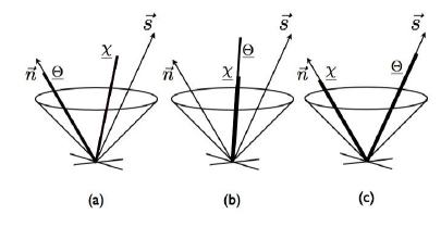
Figure 1: Illustration of relative position of particle and entropy 4-momentum (associated contra-variant vectors marked as heavy lines) with respect to the corresponding flow vectors (marked as arrows) for (a) (aberrant) Eckart model; (b) (better) Landau-Lifshitz model; (c) (congenial) regular model

4 Canonical formulation of regular theory

In order to convert the “regular” theory from the “standardised” (Eckart type) formulation we have been using so far back to its natural “canonical” (exterior differential) formulation, in which it was originally presented [7, 8] we need to introduce the entropy transport vector, $\sigma^{\mu}$, as defined with respect to the conserved particle (Eckart’s preferred) reference frame by

$$\sigma^{\mu}=s\big{(}c^{\mu}+c^{\nu}b_{\nu}b^{\mu})\;\;,\qquad c^{\nu}b_{\nu}=0\;\;.$$ (17)

We also need to introduce the resistivity scalar $Z$ defined by

$$Z=\frac{1}{\kappa(b^{\mu}c_{\mu})^{2}}\;\;.$$ (18)

In terms of these quantities, the complete set of equations of the “regular” model may be written (in a version reminiscent of the four historic Maxwell equations) as a pair of exterior differential equations

$$2n^{\nu}\nabla_{[\nu}\chi_{\mu]}+Zs^{\nu}\Theta_{\nu}\sigma_{\mu}=0\;\;,$$ (19)

and

$$2s^{\nu}\Big{(}\nabla_{[\nu}\Theta_{\mu]}+Z\sigma_{[\nu}\Theta_{\mu]}\Big{)}=0\;\;,$$ (20)

(where square brackets denote antisymmetrisation of indices), together with the pair of interior differential equations

$$\nabla_{\nu}n^{\nu}=0\;\;,\qquad\nabla_{\nu}s^{\nu}=Z\sigma^{\nu}\sigma_{\nu}\;\;.$$ (21)

In this theory it is manifest that (like the Landau-Lifshitz theory, but unlike the Eckart theory) the “regular” theory treats the conserved particle current and the entropy current on the same footing in the non-dissipative limit $Z\rightarrow 0$. The form of the differential equations (19), (20), (21) holds not only for the “regular” category, but but also more generally for the extended category of (in general “anomalous”) conducting fluid models of variational type referred to above [7, 8], but in these more general models the algebraic defining relations will no longer have the simple form for the regular subcategory in Section 3.

Editor’s note: A review of pertinent progress since this article was originally written [13] has been provided by Lopez-Monsalo and Andersson [14].

References

- [1] C. Eckart, Phys. Rev. 58, 919, (1940)
- [2] S. Weinberg, Gravitation and Cosmology, p 567 (Wiley, New York, 1972)
- [3] C. Cattaneo, C.R. Acad. Sci. Paris 247, 431 (1958)
- [4] M.C. Glaviano and D.J. Raymond, Astroph. J. 243, 271, (1981)
- [5] W.A. Hiscock and W.L. Lindblom, Phys. Rev. D 31, 725, (1985)
- [6] L. Landau and E. M. Lifshitz, Fluid Mechanics, 127 (Addision-Wesley, Reading, Mass, 1958)
- [7] B. Carter, in Journeé Relativistes 1976 (ed. Cahen, Debever, Geheniau) 12-27 (Université Libre de Bruxelles, 1976); in A Random Walk in Relativity and Cosmology (ed. Dadhich, Krishna Rao, Vishveshwara) 48-65 (Wiley Eastern, Bombay, 1985)
- [8] B. Carter, in Relativistic Fluid Mechanics (ed. M Anile and Y. Choquet–Bruhat) 1-64 (Springer, Noto, 1987)
- [9] S. Weinberg, Astrop. J. 168, 175, (1971)
- [10] I. Müller, Z. Physik, 198, 329, (1967)
- [11] W. Israel, Ann. Phys. N.Y. 100, 310, (1976)
- [12] J.S. Stewart, Proc. Roy. Soc. (Lond.) A 357, 59 (1977)
- [13] B. Carter in Proc. 5th Marcel Grossmann Meeting (Perth, August 1988), ed. D.G. Blair & M.J. Buckingham (World Scientific, Singapore, 1989) 1187-1197.
- [14] C.S. Lopez-Monsalvo, N. Andersson, Proc. Roy. Soc. (Lond.) A 467, 738 (2011) [arXiv:1107.0165]