Tagged particle diffusion in one-dimensional gas with Hamiltonian dynamics

Abstract

We consider a one-dimensional gas of hard point particles in a finite box that are in thermal equilibrium and evolving under Hamiltonian dynamics. Tagged particle correlation functions of the middle particle are studied. For the special case where all particles have the same mass, we obtain analytic results for the velocity auto-correlation function in the short time diffusive regime and the long time approach to the saturation value when finite-size effects become relevant. In the case where the masses are unequal, numerical simulations indicate sub-diffusive behaviour with mean square displacement of the tagged particle growing as $t/\ln(t)$ with time $t$. Also various correlation functions, involving the velocity and position of the tagged particle, show damped oscillations at long times that are absent for the equal mass case.

1 Introduction

Observing the dynamics of a single tagged particle in a many particle system constitute a simple way of probing the complex dynamics of an interacting many body system and has been studied both theoretically jepsen65 ; harris65 ; lebowitz67 ; lebowitz72 and experimentally hahn96 ; wei00 ; lutz04 . Much of the theoretical studies on tagged particle diffusion have focussed on one-dimensional systems and discussed two situations where the microscopic particle dynamics is (i) Hamiltonian jepsen65 ; lebowitz67 ; lebowitz72 or (ii) stochastic harris65 ; beijeren83 ; kollman03 ; lizana08 ; gupta07 ; barkai09 ; barkai10 .

For systems with Hamiltonian dynamics, the evolution of the system is completely deterministic and all the randomness in the system is due to the randomness in the initial condition. One of the earliest result for systems with Hamiltonian evolution is that of Jepsen jepsen65 on tagged particle diffusion in a one-dimensional hard particle gas of elastically colliding particles of equal masses. For an infinite system at a fixed density of particles Jepsen showed that the mean square deviation (MSD) of a tagged particle from its initial position grows linearly with time $t$. He obtained an explicit expression for the diffusion constant and the related velocity autocorrelation function (VAF). This was done by exploiting the fact that when two particles of equal mass collide elastically in a one-dimensional system, their velocities are exchanged; if we ignore tags on particles, this is is equivalent to the particles passing through each other without colliding, simplifying the dynamics.

For a finite system, with $N$ particles, there must be corrections to Jepsen’s result, since the MSD must saturate at long time (to a value that depends on the size of the system). This situation has been extensively studied for stochastic dynamics beijeren83 ; kollman03 ; lizana08 ; gupta07 ; barkai09 ; barkai10 but not much for the Hamiltonian case evans79 ; kasper85 ; lebowitz72 . Lebowitz and Sykes lebowitz72 considered finite size effects for some special initial conditions. In this paper we consider Boltzmann distributed initial coniditions. The first objective of this paper is to obtain analytical expressions for the VAF that are valid over the entire regime: both $t<<N$ (à la Jepsen) and $t>>N.$

If the particle masses are not all the same in a hard particle gas, there are no analytical results. Since the dynamics are expected to be ergodic, the correlation functions should be very different from those of the equal mass particle gas. Indeed, a simulation study marro85 of a gas where odd and even numbered particles have different masses suggested that the decay of the VAF with time $t$ in this model was as $\sim t^{-\delta}$ with $\delta\lesssim 1$ which is completely different from the Jepsen result ($\sim t^{-3}$). If this is correct, it would imply that tagged particle motion is superdiffusive in this system. The second objective of this paper is to accurately obtain the decay of the VAF and other correlation functions for a hard particle gas with unequal masses, to see if tagged particle motion is superdiffusive. We perform simulations on a one-dimensional gas with alternating masses. To ascertain how robust the numerical results are we also do simulations with randomly chosen masses.

Although there has been considerable work on the (hydro)dynamics of one dimensional hard particle gas and other systems in the context of heat conduction narayan02 , this involves the propagation of conserved quantities as a function of position and time without reference to the identity of each particle. This changes things considerably: for instance, conserved quantities propagate ballistically for an equal mass hard particle gas, resulting in a thermal conductivity proportional to $N,$ while tagged particle dynamics in the same system is diffusive. Thus here we approach the dynamics from a perspective that is different from the heat conduction literature.

In sec. (2) we define the model and dynamics and give analytic results for the VAF in the special case where all masses are equal. In sec. (3) we present the simulation results for the VAF and other correlation functions for the general case where masses are not all equal. We summarize our results in Sec. 4. Some details of the calculation are given in Appendix A.

2 Analytic results for equal mass hard-particle gas

Here we consider a gas of $N=2M+1$ point particles in a one-dimensional box of length $L$. The particles interact with each other through hard collisions conserving energy and momentum. The Hamiltonian of the system thus consists of only kinetic energy. All the particles have the same mass $m.$ In any interparticle collision, the two colliding particles exchange velocities. When a terminal particle collides with the adjacent wall, its velocity is reversed. The initial state of the system is drawn from the canonical ensemble at temperature $T$. Therefore, the initial positions of the particles are uniformly distributed in the box. Let $x_{i}$ be the position of the $i$-th particle measured with respect to the “left” wall, and $0<x_{1}<x_{2}<\dotsb<x_{N-1}<x_{N}<L$. The initial velocities of the particles are choosen independently from the Gaussian distribution with zero mean and a variance $\overline{v}^{2}=k_{B}T/m$.

By exchanging the identities of the particles emerging from collisions, one can effectively treat the system as non-interacting jepsen65 . In the non-interacting picture, each particle executes an independent motion. The particles pass through each other when they ‘collide’ and reflect off the walls at $x=0$ and $x=L.$ The initial condition is that each particle is independently chosen from the single particle distribution $p(x,v)=L^{-1}(2\pi\bar{v}^{2})^{-1/2}e^{-v^{2}/2\bar{v}^{2}}$, where $\bar{v}^{2}=k_{B}T/m$. To find the VAF of the middle particle in the interacting-system from the dynamics of the non-interacting system, we note that there are two possibilities in the non-interacting picture: (1) the same particle is the middle particle at both times $t=0$ and $t$, or (2) two different particles are at the middle position at times $t=0$ and $t$ respectively. We denote the VAF corresponding to these two cases by $\langle v_{M}(0)v_{M}(t)\rangle_{1}$ and $\langle v_{M}(0)v_{M}(t)\rangle_{2}$ respectively. The complete VAF is given by $\langle v_{M}(0)v_{M}(t)\rangle=\langle v_{M}(0)v_{M}(t)\rangle_{1}+\langle v_{M}(0)v_{M}(t)\rangle_{2}$. We now present a physically motivated derivation of these two quantities. A direct derivation and some more details are given in an appendix.

We first define a few quantities. The probability density for a (non-interacting) particle to be at $x$ at time $t=0$ and $y$ at time $t$ is

$$P(x,y;t) =\frac{1}{L\sqrt{2\pi}\overline{v}t}\sum_{n=-\infty}^{\infty}\Biggl{\{}\exp\left[-\frac{(2nL+y-x)^{2}}{2\overline{v}^{2}t^{2}}\right]+\exp\left[-\frac{(2nL-y-x)^{2}}{2\overline{v}^{2}t^{2}}\right]\Biggr{\}}$$

$$=\frac{1}{L^{2}}\sum_{k=-\infty}^{\infty}\cos\frac{\pi kx}{L}\cos\frac{\pi ky}{L}\exp[-\overline{v}^{2}t^{2}k^{2}\pi^{2}/(2L^{2})].$$ (1)

The first line is easily obtained by realizing that, for a free particle in an infinite box with a Gaussian velocity distribution, the corresponding probability density is $(L\overline{v}t\sqrt{2\pi})^{-1}\exp[-(x-y)^{2}/(2\overline{v}^{2}t^{2})],$ and the boundaries at $x=0$ and $L$ set up an infinite sequence of image sources. The second line is obtained using the Poisson resummation formula or by realizing that with $\tau=t^{2},$ the first expression satisfies $\partial_{\tau}P=-\overline{v}^{2}\partial_{y}^{2}P$ with initial condition $P(x,y,0)=\delta(x-y)/L$ and boundary conditions $\partial_{y}P(x,0,\tau)=\partial_{y}P(x,L,\tau)=0,$ and expressing this in terms of the eigenfunctions of the Laplacian. As a variant of Eq. (1) we also define the function

$$P_{-}(x,y;t) =\frac{1}{L\sqrt{2\pi}\overline{v}t}\sum_{n=-\infty}^{\infty}\biggl{\{}\exp\left[-\frac{(2nL+y-x)^{2}}{2\overline{v}^{2}t^{2}}\right]-\exp\left[-\frac{(2nL-y-x)^{2}}{2\overline{v}^{2}t^{2}}\right]\biggr{\}}$$

$$=\frac{1}{L^{2}}\sum_{k=-\infty}^{\infty}\sin\frac{\pi kx}{L}\sin\frac{\pi ky}{L}\exp[-\overline{v}^{2}t^{2}k^{2}\pi^{2}/(2L^{2})].$$ (2)

In terms of these functions, the correlation function $\langle v_{M}(0)v_{M}(t)\rangle_{1}$ can be found by picking one of the non-interacting particles at random, calculating the probability that it goes from $(x,0)$ to $(y,t)$ and that it is in the middle at both $t=0$ and $t,$ multiplying by $v(0)v(t)$ and integrating over $x$ and $y.$ The multiplication by $v(0)v(t)$ is equivalent to inserting a factor of $(2nL+y-x)^{2}/t^{2}$ in the first term of the first line of Eq.(1) and a factor of $-(2nL-y-x)^{2}/t^{2}$ in the second term, since they correspond to even and odd number of reflections respectively. Thus one obtains the normalized correlation function (see appendix)

$$C_{vv}^{(1)}=\frac{\langle v_{M}(0)v_{M}(t)\rangle_{1}}{\bar{v}^{2}}=N\int_{0}^{L}dx\int_{0}^{L}dy~{}P_{N}^{(1)}(x,y,t)~{}\partial_{\overline{v}}[\overline{v}P_{-}(x,y,t)],$$ (3)

where $P_{N}^{(1)}(x,y,t)$ is the probability that there are an equal number of particles to the left and right of $x$ and $y$ at $t=0$ and $t$ respectively.

Turning to $\langle v_{M}(0)v_{M}(t)\rangle_{2},$ we pick two particles at random at time $t=0,$ calculate the probability that they go from $(x,0)$ to $(y,t)$ and $(\tilde{x},0)$ to $(\tilde{y},t),$ that there are an equal number of particles on both sides of $x$ and $\tilde{y}$ at $t=0$ and $t$ respectively, multiplying by $v(0)\tilde{v}(t)$ and integrating with respect to $x,y,\tilde{x},\tilde{y}$. From Eq.(1), multiplying $P(x,y,t)$ by $v(0)$ is equivalent to inserting a factor of $(2nL+y-x)/t$ and $(2nL-y-x)/t$ in front of the first and second terms respectively in the first line. Also, multiplying $P(\tilde{x},\tilde{y},t)$ by $\tilde{v}(t)$ is equivalent to inserting a factor of $(2nL+\tilde{y}-\tilde{x})/t$ and $-(2nL-\tilde{y}-\tilde{x})/t$ in front of the two terms. Converting these factors to appropriate derivatives, we have for the normalized correlation function

$$C_{vv}^{(2)}=N(N-1)\idotsint dxd\tilde{x}dyd\tilde{y}~{}P_{N}^{(2)}(x,\tilde{x},y,\tilde{y},t)\bigl{[}\overline{v}t~{}\partial_{x}P(x,y,t)\bigr{]}\bigl{[}-\overline{v}t~{}\partial_{\tilde{y}}P(\tilde{x},\tilde{y})\bigr{]},$$ (4)

where $P^{(2)}_{N}(x,y,\tilde{x},\tilde{y},t)$ is the probability that there are an equal number of particles on both sides of $x$ and $\tilde{y}$ at $t=0$ and $t$ respectively, given that there is one particle at $(\tilde{x},0)$ and at $(y,t).$

To proceed further, we need the expressions for $P^{(1,2)}_{N}$. For this we define $p_{-+}(x,y;t)$ as the probability that a particle is to the left of $x$ at $t=0$ and to the right of $y$ at time $t$. Let $p_{+-}$, $p_{--}$ and $p_{++}$ be similarly defined. Thus

$$p_{-+}(x,y;t)=\int_{0}^{x}dx^{\prime}\int_{y}^{L}dy^{\prime}P(x^{\prime},y^{\prime};t)~{},$$

$$p_{+-}(x,y;t)=\int_{x}^{L}dx^{\prime}\int_{0}^{y}dy^{\prime}P(x^{\prime},y^{\prime};t)~{},$$

$$p_{--}(x,y;t)=\int_{0}^{x}dx^{\prime}\int_{0}^{y}dy^{\prime}P(x^{\prime},y^{\prime};t)~{},$$

$$p_{++}(x,y;t)=\int_{x}^{L}dx^{\prime}\int_{y}^{L}dy^{\prime}P(x^{\prime},y^{\prime};t)~{}.$$ (5)

In terms of the expressions defined in Eqs.(5), it is straightforward to see that

$$P_{N}^{(1)}(x,y,t) =\int_{-\pi}^{\pi}\frac{d\phi}{2\pi}\int_{-\pi}^{\pi}\frac{d\theta}{2\pi}~{}\Bigl{[}p_{++}e^{i\phi}+p_{--}e^{-i\phi}+p_{+-}e^{i\theta}+p_{-+}e^{-i\theta}\Bigr{]}^{N-1}$$

$$=\frac{2}{(2\pi)^{2}}\int_{-\pi/2}^{\pi/2}d\phi\int_{-\pi}^{\pi}d\theta~{}\Bigl{[}1-(1-\cos{\phi})~{}(p_{++}+p_{--})+i\sin\phi~{}(p_{++}-p_{--})$$

$$~{}~{}~{}~{}~{}~{}~{}~{}~{}~{}~{}~{}~{}~{}~{}~{}~{}~{}~{}~{}~{}~{}~{}~{}~{}~{}~{}~{}~{}~{}~{}~{}~{}~{}~{}-(1-\cos{\theta})~{}(p_{+-}+p_{-+})+i\sin\theta~{}(p_{+-}-p_{-+})\Bigr{]}^{N-1}~{},$$ (6)

where we used the identity $p_{++}+p_{+-}+p_{-+}+p_{--}=1$, the fact that $N-1$ is even and the integrands are unchanged if $\theta,\phi$ are increased by $\pi$. The angular integrals enforce the conditions that if $m+n$ particles are to right of $x$ at time $t=0,$ of which $n$ particles cross from right to left in time $t,$ then $n$ particles cross from left to right and $m$ particles remain on the left, so that the number of particles on both sides of $x$ at time $t=0$ and $y$ at time $t$ is $m+n$ (see appendix for more details). From Eqs.(3) and (6) we get

$$C_{vv}^{(1)} =N\frac{2}{(2\pi)^{2}}\int_{0}^{L}dx\int_{0}^{L}dy\int_{-\pi/2}^{\pi/2}d\phi\int_{-\pi}^{\pi}d\theta~{}\partial_{\bar{v}}[\overline{v}P_{-}(x,y,t)]$$

$$\qquad\times\Bigl{[}1-(1-\cos{\phi})~{}(p_{++}+p_{--})+i\sin\phi~{}(p_{++}-p_{--})$$

$$\qquad\qquad-(1-\cos{\theta})~{}(p_{+-}+p_{-+})+i\sin\theta~{}(p_{+-}-p_{-+})\Bigr{]}^{N-1}~{}.$$ (7)

Using similar arguments as used for Eq.(6) (see appendix), one can write

$$P_{N}^{(2)}(x,y,\tilde{x},\tilde{y},t) =\int_{-\pi}^{\pi}\frac{d\phi}{2\pi}\int_{-\pi}^{\pi}\frac{d\theta}{2\pi}~{}\Bigl{[}p_{++}(x,\tilde{y})e^{i\phi}+p_{--}(x,\tilde{y})e^{-i\phi}$$

$$\qquad\qquad\qquad+p_{+-}(x,\tilde{y})e^{i\theta}+p_{-+}(x,\tilde{y})e^{-i\theta}\Bigr{]}^{N-2}\,\psi(\theta,\phi)$$

$$=\frac{2}{(2\pi)^{2}}\int_{-\pi/2}^{\pi/2}d\phi\int_{-\pi}^{\pi}d\theta~{}\Bigl{[}1-(1-\cos{\phi})~{}(p_{++}+p_{--})$$

$$\qquad\qquad+i\sin\phi~{}(p_{++}-p_{--})-(1-\cos{\theta})~{}(p_{+-}+p_{-+})$$

$$\qquad\qquad\qquad+i\sin\theta~{}(p_{+-}-p_{-+})\Bigr{]}^{N-2}~{}\psi(\theta,\phi)~{}.$$ (8)

where

$$\psi(\theta,\phi)=\begin{cases}e^{-i\phi}&\text{for}~{}~{}x>\tilde{x}~{},y<\tilde{y}\\ e^{-i\theta}&\text{for}~{}~{}x>\tilde{x}~{},~{}y>\tilde{y}\\ e^{i\phi}&\text{for}~{}~{}x<\tilde{x}~{},~{}y>\tilde{y}\\ e^{i\theta}&\text{for}~{}~{}x<\tilde{x}~{},~{}y<\tilde{y}~{}.\end{cases}$$ (9)

Using the second line of Eq.(1) for $P(x,y,t)$ and $P(\tilde{x},\tilde{y},t),$ integrating over $y$ and $\tilde{x},$ and comparing to the second line of Eq.(2) we obtain

$$C_{vv}^{(2)}=-N(N-1)\overline{v}^{2}t^{2}\frac{2}{(2\pi)^{2}}\int_{0}^{L}dx\int_{0}^{L}d\tilde{y}\int_{-\pi/2}^{\pi/2}d\phi\int_{-\pi}^{\pi}d\theta~{}P_{-}^{2}(x,\tilde{y},t)(2\cos\phi-2\cos\theta)\\ \times\Bigl{[}1-(1-\cos{\phi})~{}(p_{++}+p_{--})+i\sin\phi~{}(p_{++}-p_{--})-(1-\cos{\theta})~{}(p_{+-}+p_{-+})+i\sin\theta~{}(p_{+-}-p_{-+})\Bigr{]}^{N-2}~{}.$$ (10)

2.1 Short time regime

When $\bar{v}t<<L,$ the tagged particle does not feel the effect of the walls and we can make the following approximations

$$P(x,y,t)=P_{-}(x,y,t)=\frac{1}{\sqrt{2\pi}\overline{v}tL}\exp\left[-\frac{(y-x)^{2}}{2\bar{v}^{2}t^{2}}\right]~{}.$$ (11)

In this limit the expressions for $p_{-+}$, etc. given in Eq. (5) also simplify by using Eq. (11) and taking the limits of the $y^{\prime}$ integral to be from $y$ to $\infty$ for $p_{-+},p_{++}$ and from $-\infty$ to $y$ for $p_{+-},p_{--}$. We then get

$$Np_{++}(x,y;t) \approx\frac{\rho}{\sqrt{2\pi}\bar{v}t}\int_{x}^{L}dx^{\prime}\int_{y}^{\infty}dy^{\prime}~{}e^{-{(y^{\prime}-x^{\prime})^{2}}/{2\bar{v}^{2}t^{2}}}~{}\approx\frac{N}{2}-\frac{\lambda z_{+}}{2}-\lambda q(z_{-})~{},$$

$$Np_{--}(x,y;t) \approx\frac{\rho}{\sqrt{2\pi}\bar{v}t}\int_{0}^{x}dx^{\prime}\int_{-\infty}^{y}dy^{\prime}~{}e^{-{(y^{\prime}-x^{\prime})^{2}}/{2\bar{v}^{2}t^{2}}}\approx\frac{N}{2}+\frac{\lambda z_{+}}{2}-\lambda q(z_{-})~{},$$

$$Np_{+-}(x,y;t) \approx\frac{\rho}{\sqrt{2\pi}\bar{v}t}\int_{x}^{L}dx^{\prime}\int_{-\infty}^{y}dy^{\prime}~{}e^{-{(y^{\prime}-x^{\prime})^{2}}/{2\bar{v}^{2}t^{2}}}\approx-\frac{\lambda z_{-}}{2}+\lambda q(z_{-})~{},$$

$$Np_{-+}(x,y;t) \approx\frac{\rho}{\sqrt{2\pi}\bar{v}t}\int_{0}^{x}dx^{\prime}\int_{y}^{\infty}dy^{\prime}~{}e^{-{(y^{\prime}-x^{\prime})^{2}}/{2\bar{v}^{2}t^{2}}}\approx\frac{\lambda z_{-}}{2}+\lambda q(z_{-})~{},$$ (12)

$${\rm where}~{}z_{+} =\frac{x+y-L}{\bar{v}t},~{}z_{-}=\frac{x-y}{\bar{v}t}~{},\lambda=\rho\bar{v}t~{}~{}\text{with}~{}\rho=N/L,$$

$${\rm and}~{}q(z_{-}) =\frac{e^{-z_{-}^{2}/2}}{\sqrt{2\pi}}+\frac{z_{-}}{2}\mbox{Erf}(z_{-}/\sqrt{2})~{}$$ (13)

Hence we get $N(p_{++}+p_{--})=N-2\lambda q(z_{-}),~{}N(p_{++}-p_{--})=-\lambda z_{+},~{}N(p_{+-}+p_{-+})=2\lambda q(z_{-}),~{}N(p_{+-}-p_{-+})=-\lambda z_{-}$ . Using these in Eqs. (7) and (10), and changing variables from $x_{0},x_{t}$ and $x_{0},\tilde{x}_{t}$ to $z_{+},z_{-}$ we get, for large $N$

$$C_{vv}^{(1)}(t) =\frac{\lambda}{\sqrt{2\pi}(2\pi)^{2}}\int_{-\infty}^{\infty}dz_{+}\int_{-\infty}^{\infty}dz_{-}z_{-}^{2}e^{-z_{-}^{2}/2}\int_{-\pi/2}^{\pi/2}d\phi\int_{-\pi}^{\pi}d\theta\,$$

$$\qquad\qquad\times e^{-N(1-\cos\phi)}e^{-i\lambda z_{+}\sin\phi}e^{-2\lambda q(z_{-})(1-\cos\theta)}e^{-i\lambda z_{-}\sin\theta}~{},$$

$$C_{vv}^{(2)}(t) =-\frac{\lambda^{2}}{4\pi^{3}}\int_{-\infty}^{\infty}dz_{+}\int_{-\infty}^{\infty}dz_{-}e^{-z_{-}^{2}}\int_{-\pi/2}^{\pi/2}d\phi\int_{-\pi}^{\pi}d\theta~{}(\cos\phi-\cos\theta)~{}$$

$$\qquad\qquad\times e^{-N(1-\cos\phi)}e^{-i\lambda z_{+}\sin\phi}e^{-2\lambda q(z_{-})(1-\cos\theta)}e^{-i\lambda z_{-}\sin\theta}~{}.$$

For large $N$, the major contribution of the integral over $\phi$ comes from the region around $\phi=0$. Therefore, the $\phi$ integral can be performed by expanding around $\phi=0$ to make it a Gaussian integral (while extending the limits to $\pm\infty$). Subsequently, one can also perform the Gaussian integral over $z_{+}$. This leads to the following expressions:

$$C_{vv}^{(1)}(t) =\frac{1}{(2\pi)^{3/2}}\int_{-\infty}^{\infty}dz_{-}z_{-}^{2}e^{-z_{-}^{2}/2}\int_{-\pi}^{\pi}d\theta e^{-2\lambda q(z_{-})(1-\cos\theta)}e^{-i\lambda z_{-}\sin\theta}~{},$$ (14)

$$C_{vv}^{(2)}(t) =-\frac{\lambda}{2\pi^{2}}\int_{-\infty}^{\infty}dz_{-}e^{-z_{-}^{2}}~{}\int_{-\pi}^{\pi}d\theta~{}(1-\cos\theta)~{}e^{-2\lambda q(z_{-})(1-\cos\theta)}e^{-i\lambda z_{-}\sin\theta}~{}.$$ (15)

Thus we have closed form expressions of the VAF which are valid in the entire short time regime. For any value of $\lambda=\rho\overline{v}t$, these integrals can be performed numerically, and as we see from Fig. 1, the results are in excellent agreement with the numerical simulation.

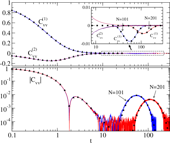
Figure 1: Plot of the separate contributions $C_{vv}^{(1)}$ and $C_{vv}^{(2)}$ to the velocity-autocorrelation function of equal mass hard-particle gas, for two different system sizes ($N=101,201$) with fixed density $\rho=1$, and $\overline{v}=1$. The solid lines correspond to the simulation data, whereas the points are from the analytical results given by Eqs. (7) and (10) for short time behaviors ($\blacktriangle$), and Eq. (26) for the long time behaviors ($\blacksquare$). In the first panel, the dashed rectangle is enlarged in the inset.

We now analyze the above expression in the large $\lambda$ limit, i.e., $(\overline{v}\rho)^{-1}\ll t.$ Together with the condition $\overline{v}t<<L$ for being in the short time regime, this means that $t$ is much larger than the typical time between interparticle collisions, i.e. outside the ballistic regime, while being much smaller than the time it takes to see finite size effects. We first make a change of variables $\sqrt{\lambda}z_{-}=z$ and $\sqrt{\lambda}\theta=x$. The integrands can then be expanded as a power series in powers of $1/\lambda$. The integrals acquire the forms:

$$C_{vv}^{(1)}(t) =\frac{1}{(2\pi)^{3/2}}\int_{-\infty}^{\infty}dz\int_{-\sqrt{\lambda}\pi}^{\sqrt{\lambda}\pi}dx\,e^{-\frac{x^{2}}{\sqrt{2\pi}}-ixz}\sum_{n=2}^{\infty}a_{n}(x,z)\lambda^{-n},$$ (16)

$$C_{vv}^{(2)}(t) =-\frac{1}{2\pi^{2}}\int_{-\infty}^{\infty}dz\int_{-\sqrt{\lambda}\pi}^{\sqrt{\lambda}\pi}dx\,e^{-\frac{x^{2}}{\sqrt{2\pi}}-ixz}\sum_{n=1}^{\infty}b_{n}(x,z)\lambda^{-n},$$ (17)

where $a_{n}(x,z)$ and $b_{n}(x,z)$ are polynomials in $x$ and $z$. For example, $a_{2}(x,z)=z^{2}$, $b_{1}(x,z)=x^{2}/2$, and so on. Now, integrating term by term (while extending the integrating limits of $x$ to $\pm\infty$) we get

$$C_{vv}^{(1)}(t) =\frac{1}{\pi}\lambda^{-2}-\frac{2(\pi-3)}{(2\pi)^{3/2}}\lambda^{-3}+O(\lambda^{-5}),$$ (18)

$$C_{vv}^{(2)}(t) =-\frac{1}{\pi}\lambda^{-2}-\frac{1}{(2\pi)^{3/2}}\lambda^{-3}+O(\lambda^{-4}).$$ (19)

Therefore, adding the above two results, we recover Jepsen’s result jepsen65

$$C_{vv}(t)=-\frac{(2\pi-5)}{(2\pi)^{3/2}}\lambda^{-3}+O(\lambda^{-4}).$$ (20)

2.2 Long time regime

In the limit $\bar{v}t>>L$ we integrate Eqs.(5) using the second line of Eq.(1):

$$p_{--}(x,y;t) = \frac{xy}{L^{2}}+f(x,y;t)$$

$$p_{-+}(x,y;t) = \frac{x(L-y)}{L^{2}}-f(x,y;t)$$

$$p_{+-}(x,y;t) = \frac{y(L-x)}{L^{2}}-f(x,y;t)$$

$$p_{++}(x,y;t) = \frac{(L-x)(L-y)}{L^{2}}+f(x,y;t)$$ (21)

with

$$f(x,y;t)=\sum_{k\neq 0}\frac{1}{k^{2}\pi^{2}}\exp\left(-\frac{k^{2}\pi^{2}\overline{v}^{2}t^{2}}{2L^{2}}\right)\sin\left(\frac{k\pi x}{L}\right)\sin\left(\frac{k\pi y}{L}\right).$$ (22)

Expanding around $x=y=L/2$ we get to leading order $N(p_{++}+p_{--})=N[1/2+2a(t)],~{}N(p_{++}-p_{--})=-Nw_{+},~{}N(p_{+-}+p_{-+})=N[1/2-2a(t)],~{}N(p_{+-}+p_{-+})=-Nw_{-}$ , where $w_{+}=(x+y)/L-1,~{}w_{-}=(x-y)/L$ and

$$a(t)=f(L/2,L/2;t)=\sum_{k}\frac{1}{\pi^{2}(2k+1)^{2}}\exp\left[-\frac{(2k+1)^{2}\pi^{2}\overline{v}^{2}t^{2}}{2L^{2}}\right].$$ (23)

Using these and the expression of $P_{-}$ from Eq. (2) in Eqs. (7) and (10), we find the following results upto $O(1/N)$:

$$C_{vv}^{(1)}(t)= N\sum_{k}\left(1-\frac{(2k+1)^{2}\pi^{2}\overline{v}^{2}t^{2}}{L^{2}}\right)\exp\left(-\frac{(2k+1)^{2}\pi^{2}\overline{v}^{2}t^{2}}{2L^{2}}\right)$$

$$\qquad\qquad\times\frac{1}{(2\pi)^{2}}~{}\int_{-\infty}^{\infty}{dw_{+}}\int_{-\infty}^{\infty}dw_{-}\int_{-\infty}^{\infty}d\phi\int_{-\infty}^{\infty}d\theta$$

$$\qquad\qquad\times e^{-N[1/4+a(t)]\phi^{2}}e^{-iNw_{+}\phi}e^{-N[1/4-a(t)]\theta^{2}}e^{-iNw_{-}\theta}~{},$$ (24)

$$C_{vv}^{(2)}(t)= -N^{2}\left(\frac{\bar{v}t}{L}\right)^{2}\left[\sum_{k}\exp\left(-\frac{(2k+1)^{2}\pi^{2}\overline{v}^{2}t^{2}}{2L^{2}}\right)\right]^{2}$$

$$\times\frac{1}{(2\pi)^{2}}~{}\int_{-\infty}^{\infty}{dw_{+}}\int_{-\infty}^{\infty}dw_{-}\int_{-\infty}^{\infty}d\phi\int_{-\infty}^{\infty}d\theta$$

$$\times e^{-N[1/4+a(t)]\phi^{2}}e^{-iNw_{+}\phi}e^{-N[1/4-a(t)]\theta^{2}}e^{-iNw_{-}\theta}~{}(\theta^{2}-\phi^{2})~{}.$$ (25)

Performing the Gaussian integrals we find that $C_{vv}^{(2)}$ vanishes and hence to $O(1/N)$ the velocity autocorrelation is given by

$$C_{vv}(t)=C_{vv}^{(1)}(t)=\frac{2}{N}\sum_{k=1,3,5\ldots}\left(1-\frac{k^{2}\pi^{2}\overline{v}^{2}t^{2}}{L^{2}}\right)\exp\left(-\frac{k^{2}\pi^{2}\overline{v}^{2}t^{2}}{2L^{2}}\right).$$ (26)

As seen from Fig. 1, the above expression describes the numerical simulation data very well. The late time behaviour $C_{vv}(t)\sim\exp(-\pi^{2}\overline{v}^{2}t^{2}/2L^{2})$ was earlier obtained in evans79 .

3 Simulation results

As mentioned earlier, there are no analytical results when the particle masses in the one dimensional gas are not all equal. We turn to numerical simulations for such systems; the simulations also confirm the analytical results of the previous section, as shown in Figure 1. The Hamiltonian for the system is $H=\sum_{l=1}^{N}{1\over 2}m_{l}\dot{x}_{l}^{2},$ with $0<x_{1}<x_{2}\ldots<x_{N}<L.$ After an elastic collision between two neighboring particles (say $l$ and $l+1$) with velocities $v_{l}$, $v_{l+1}$ and masses $m_{l}$, $m_{l+1}$ respectively, they emerge with new velocities $v_{l}^{\prime}$ and $v_{l+1}^{\prime}$. From momentum and energy conservation we have:

$$v_{l}^{\prime} =\frac{(m_{l}-m_{l+1})}{(m_{l}+m_{l+1})}v_{l}+\frac{2m_{l+1}}{(m_{l}+m_{l+1})}v_{l+1}$$

$$v_{l+1}^{\prime} =\frac{2m_{l}}{(m_{l}+m_{l+1})}v_{l}+\frac{(m_{l+1}-m_{l})}{(m_{l}+m_{l+1})}v_{l+1}~{}.$$ (27)

Between collisions the particles move with constant velocity.

We simulate this system using an event-driven algorithm and compute the correlation functions $\langle[\Delta x(t)]^{2}\rangle$, $\langle\Delta x(t)v(0)\rangle$ and $\langle v(t)v(0)$ of the central particle, where $\Delta x(t)=x_{M}(t)-x_{M}(0)$ and $v(t)=v_{M}(t)$. The average $\langle\cdots\rangle$ is taken over initial configurations chosen from the equilibrium distribution, where the particles are uniformly distributed in the box with density $\rho=N/L$, while the velocity of each particle is independently chosen from the distribution $(m/2\pi k_{B}T)^{1/2}~{}e^{-mv^{2}/2k_{B}T}$ . Note that the three correlation functions are related to each other as

$$\frac{1}{2}\frac{d}{dt}\langle[\Delta x(t)]^{2}\rangle=\langle\Delta x(t)v(t)\rangle=\langle\Delta x(t)v(0)\rangle=\int_{0}^{t}\langle v(0)v(t^{\prime})\rangle dt^{\prime}=D(t)~{}.$$

When the tagged particle shows diffusive behaviour then $\lim_{t\to\infty}D(t)$ reaches a constant value for an infinite system and this gives the diffusion constant. On the other hand for sub-diffusion $D(t)$ vanishes as $t\to\infty$ whereas for super-diffusion it diverges.

Just as for the equal mass system, for any finite system of size $L$ there is a short time regime during which the tagged particle at the centre does not feel the effect of the boundaries and during this time, correlation functions have the same behaviour as the infinite system. The time at which the system size effects start showing up is given by $t_{\rm sat}\sim L/c_{s}$, where $c_{s}=\sqrt{3P/\rho_{m}}$ is the adiabatic sound velocity in the hard particle gas, with $P$ the pressure and $\rho_{m}$ the average mass density. For our numerical simulations, $P=\rho k_{B}T=1$ and $\rho_{m}=1,$ which gives $c_{s}=\sqrt{3}$. We now present the results for the correlation functions in the short-time and long-time regimes.

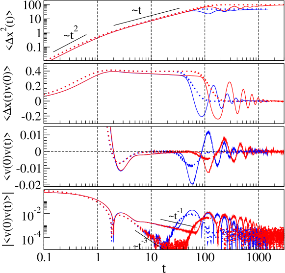
Figure 2: (color online) Various correlation functions for alternate mass hard particle gas (solid lines) with $N=101$ (blue) and $N=201$ (red) particles, density $\rho=1$ and $k_{B}T=1$. The alternate particles have masses $1.5$ and $0.5$ and in this simulation, the middle particle had mass $1.5$. The data is obtained by averaging over $10^{9}$ equilibrium initial conditions. For comparison, the correlation functions for an equal mass gas with masses $1$ is also shown (dotted lines).

In Fig. 2, we show the simulation results for the correlation functions for a one dimensional hard particle gas with masses that alternate between $1.5$ and $0.5.$ Here the data is shown for the case where the tagged particle has mass $1.5$, and similar results are obtained for the case when the tagged particle is lighter. For comparison, the results for an equal mass gas are also shown. After the expected initial ballistic regime, the MSD $\langle\Delta x^{2}(t)\rangle$ grows approximately linearly, indicating roughly diffusive motion. Simulation results of Marro and Masoliver marro85 obtained $\langle v(0)v(t)\rangle\sim-t^{-\delta}$ with $\delta\leq 1$ for the gas with alternating masses, which would imply (slightly) superdiffusive behavior. It is easiest to notice any deviations from diffusive behavior in the plot of $\langle\Delta x(t)v(0)\rangle,$ where diffusive or superdiffusive behavior would correspond to (after the ballistic regime) a horizontal or rising straight line respectively. Instead, Figure 2 shows that $\langle\Delta x(t)v(0)\rangle$ decreases as $t$ is increased beyond the ballistic regime, implying subdiffusive behavior. This is seen more clearly in Fig. (3) where we observe the dependence $\langle\Delta x(t)v(0)\rangle\sim a/(b+\ln t)$. This would correspond to an MSD whose leading part in this regime is $\sim t/\ln t$ and a VAF $\sim-1/(t\ln^{2}t)$. As seen in Fig. (2) the logarithmic corrections are difficult to observe in the MSD and VAF. The smallness of the deviation from diffusive behavior implies that the apparently linear dependence of $\langle\Delta x(t)v(0)\rangle$ on $\ln t$, observed in marro85 , is nevertheless consistent with the above observed form for small $\ln t$. However we note that the linear logarithmic dependence on time as proposed in marro85 cannot be valid at large times – and therefore our form is more appropriate. Other functional forms for are also possible. For instance, $\langle\Delta x(t)v(0)\rangle\sim t^{-\alpha}$ with a very small $\alpha$ would also imply the subdiffusive behaviour $\langle\Delta x^{2}(t)\rangle\sim t^{1-\alpha}$.

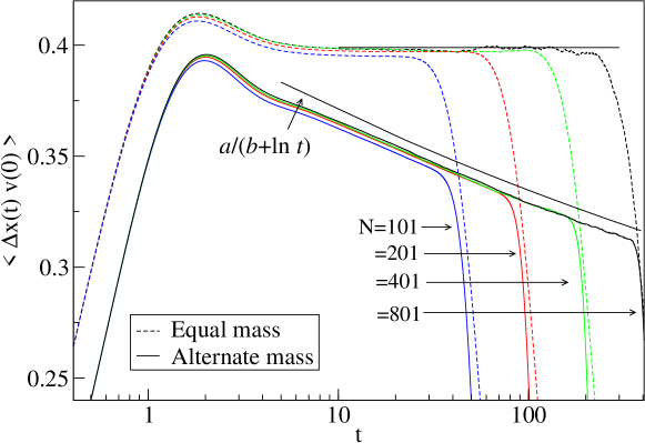
Figure 3: Plot of $D(t)=\langle\Delta x(t)v(0)\rangle$ for the alternate mass gas for various system sizes. We see clearly the logarithmic decay of the diffusion constant. The parameters for the shown funciton are $a=8$ and $b=19$. For comparision we also show the corresponding equal mass data (dashed line) which shows saturation to the expected Jepsen value $1/\sqrt{2\pi}\approx 0.4$.

At long times, the effect of finite size of the box sets in and the MSD saturates: $\langle[x(t)-x(0)]^{2}\rangle\rightarrow 2\langle[x(t)-L/2]^{2}\rangle,$ which can be easily evaluated in equilibrium to be $L^{2}/(2N),$ independent of the particle masses in the gas. We observe this in Fig. (2). The main difference between the equal mass and alternate mass systems is that the MSD for the equal mass case approaches its saturation value without oscillations, while for alternate mass case there are damped oscillations as saturation is approached, while always remaining below the MSD for the equal mass case. The oscillations in the alternate mass system also show up in the other two correlation functions.

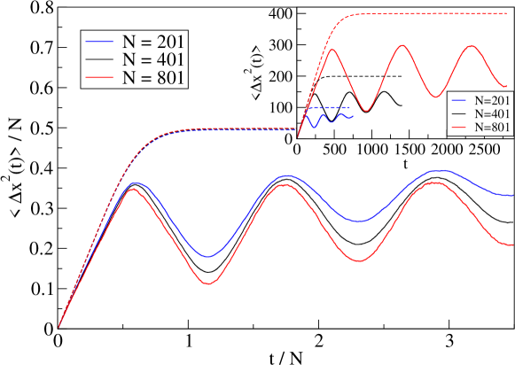
Figure 4: Scaled plot of MSD as a function of time for three system sizes $N=201,401,801$ for the alternate mass case with fixed density $\rho=1$ and other parameters as in Fig. (2). The inset shows the unscaled data. The saturation value for the scaled plot is at $0.5$.

The oscillations in the MSD are seen more clearly in Fig. 4, where the data is plotted differently. The period of oscillation is proportional to $N,$ in agreement with our discussion earlier in this section where they were ascribed to sound waves reflecting from the boundary, which takes a time $\sim L/c_{s}.$ However, the amplitude of the oscillations does not show a simple scaling with $N;$ it is clear from the figure that they are damped out in fewer cycles for smaller $N,$ making it impossible to collapse the data onto a single curve by rescaling the vertical axis.

To check for the robustness of our results we have also performed simulations of a gas with random distribution of masses. Each particle was assigned a mass from a uniform distribution between $0.5$ and $1.5$. We looked at tagged-particle correlations of the central particle whose mass was fixed at $0.5$. The correlations fluctuate between different mass realizations and we took an average over $32$ realizations. The results are plotted in Fig. (5) where we see the same qualitative features as for the alternate mass case.

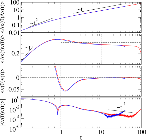
Figure 5: Various correlation functions (in the short-time regime) for random mass hard particle gas with $N=101$ and $N=201$ particles and density $\rho=1$. The mass of the middle particle was always taken to be 0.5 and the results are an average over $32$ different random mass realizations.

4 Summary

We have studied tagged particle correlations of the middle particle in a system of $N$ hard point particles confined in a one-dimensional box of length $L$ and in thermal equilibrium. For the case where the masses of all particles are equal we obtained analytic results for the finite-size velocity auto-correlation function using the approach of Jepsen. We have presented a somewhat simpler and physically motivated calculation of the velocity auto-correlation function and obtained closed form expressions valid at both short times (including the ballistic and diffusive regimes) and long times (when finite size effects show up). While here we have only presented results for the velocity auto-correlations, it is straightforward to obtain other correlation functions using our approach.

Next we have presented simulation results for the case of a hard-point gas where the particles have unequal masses. Two cases are studied, one where particles have alternate masses and the other where the masses are random. In both cases we find that the behaviour of correlation functions is qualitatively different from the equal mass case. The correlation $\langle\Delta x(t)v(0)\rangle$ does not saturate to a constant (expected for a diffusive behaviour) and instead shows a slow decay consistent with the form $\langle\Delta x^{2}(t)\rangle\sim t/\ln t$. Correspondingly the VAF decays as $\sim 1/(t\ln^{2}t)$ which is completely different from the equal mass form $\sim 1/t^{3}$. This indicates that tagged-particle motion is sub-diffusive. However it is difficult to see this sub-diffusive behaviour directly in the mean square displacement of the tagged particle since the deviation from linear time-dependence is small. These results are surprising since simulations with other interacting systems such as Lennard-Jones gases have found diffusive motion and $1/t^{3}$ decay of the velocity auto-correlation function bishop81 . Understanding this difference as well as studying tagged particle motion in other interacting systems and higher dimensional systems remain interesting open problems.

Appendix A Details of calculation

In this appendix, we provide a more detailed calculation of the velocity autocorrelation function for the hard particle gas of equal mass. This is an alternative to the derivation of some of the key equations in this paper. To compute $\langle v_{M}(0)v_{M}(t)\rangle_{1}$, we pick at time $t=0$ one of the non-interacting particles at random from the distribution $p(x_{0},v_{0})$. At time $t$ let the position and velocity of the particle be given by $x_{t}(x_{0},v_{0})$ and $v_{t}(x_{0},v_{0})$ respectively. We then calculate the probability, $P_{N}^{(1)}(x_{0},x_{t})$, that it has an equal number of particles to its left and right at both the initial and final times, i.e., at $t=0$ and $t$. For $\langle v_{M}(0)v_{M}(t)\rangle_{2}$, we pick two non-interacting particles from the distribution $p(x_{0},v_{0})~{}p(\tilde{x}_{0},\tilde{v}_{0})$ and let them evolve to $x_{t},v_{t}$ and $\tilde{x}_{t},\tilde{v}_{t}$ respectively. We then calculate the probability $P_{M}^{(2)}(x_{0},\tilde{x}_{t})$ that at time $t=0$, the first particle $x_{0}$ is the middle particle while at time $t$ the second particle $\tilde{x}(t)$ is the middle particle. The normalized VAF is thus given by:

$$C_{vv}^{(1)}(t) =\frac{\langle v_{M}(0)v_{M}(t)\rangle_{1}}{\bar{v}^{2}}=\frac{N}{\bar{v}^{2}}\int_{0}^{L}\frac{dx_{0}}{L}\int_{-\infty}^{\infty}\frac{dv_{0}}{\sqrt{2\pi}\,\overline{v}}e^{-v_{0}^{2}/2\overline{v}^{2}}\,v_{0}v_{t}\,P_{N}^{(1)}(x_{0},x_{t},t)~{},$$ (28)

$$C_{vv}^{(2)}(t) =\frac{\langle v_{M}(t)v_{M}(0)\rangle_{2}}{\bar{v}^{2}}$$

$$=\frac{N(N-1)}{\bar{v}^{2}}\idotsint\frac{dx_{0}}{L}\frac{d\tilde{x}_{0}}{L}\frac{dv_{0}d\tilde{v}_{0}}{2\pi\overline{v}^{2}}\,v_{0}\tilde{v}_{t}\,e^{-(v_{0}^{2}+\tilde{v}_{0}^{2})/2\overline{v}^{2}}~{}P_{N}^{(2)}(x_{0},x_{t},\tilde{x}_{0},\tilde{x}_{t},t)~{}.$$ (29)

These forms together with the explicit expressions of $P_{N}^{(1),(2)}$ discussed below, agree with those given in lebowitz72 . We now make a change of variables from $x_{0},v_{0}$ to $x_{0},x_{t}$ in Eq. (28) and from $x_{0},v_{0},\tilde{x}_{0},\tilde{v}_{0}$ to $x_{0},x_{t},\tilde{x}_{0},\tilde{x}_{t}$ in Eq. (29).

In the non-interacting picture, $x_{t}$ and $v_{t}$, as well as the number of collisions $m$, suffered by the particle with the walls upto time $t$, are completely determined by the initial configuration $(x_{0},v_{0})$. The number of collisions with the wall is given by

$$m=\begin{cases}\displaystyle\left\lfloor\frac{x_{0}+v_{0}t}{L}\right\rfloor&\quad\text{if}~{}v_{0}>0,\\[8.53581pt] \displaystyle\left\lfloor\frac{L-x_{0}-v_{0}t}{L}\right\rfloor&\quad\text{if}~{}v_{0}<0~{},\end{cases}$$ (30)

where $\lfloor x\rfloor$ is the integral part of $x$. When $m$ is even, we have $v_{t}=v_{0}$ whereas $v_{t}=-v_{0}$ for odd $m$. The final position $x_{t}$ is given by one of the following relations depending on $m$ and $v_{0}$. When $m$ is even, we have $x_{0}+v_{0}t=mL+x_{t}$ for $v_{0}>0$ and $L-x_{0}-v_{0}t=mL+L-x_{t}$ for $v_{0}<0$. On the other hand for odd $m$ we get $x_{0}+v_{0}t=mL+L-x_{t}$ for $v_{0}>0$ and $L-x_{0}-v_{0}t=mL+x_{t}$ for $v_{0}<0$. Combining all these four cases, we can write $x_{0}+v_{0}t=2nL\pm x_{t}$. Here $n=m/2$ and $-m/2$ respectively for the first two cases where $m$ is even and the plus sign is taken. For the last two cases, where $m$ is odd, $n=(m+1)/2$ and $-(m+1)/2$ respectively and the minus sign is taken. In other words, for a given values of $x_{0}$ and $v_{0}$ in the relations $x_{0}+v_{0}t=2nL\pm x_{t}$ and $v_{t}=\pm v_{0}$, the values of $n$ and $x_{t}$, and the signs taken from the $\pm$ are uniquely determined. Therefore, inserting the term $[\delta(x_{0}+v_{0}t-2nL-x_{t})\delta(v_{t}-v_{0})+\delta(x_{0}+v_{0}t-2nL+x_{t})\delta(v_{t}+v_{0})]$ in the integrand of Eq. (28) while integrating over $x_{t}$ and $v_{t}$, and summing over all integer values of $n$, does not change the result, i.e.,

$$\langle v_{M}(t)v_{M}(0)\rangle_{1}=N\int_{0}^{L}dx_{t}\int_{-\infty}^{\infty}dv_{t}\sum_{n=-\infty}^{\infty}\int_{0}^{L}\frac{dx_{0}}{L}\int_{-\infty}^{\infty}\frac{dv_{0}}{\sqrt{2\pi}\,\overline{v}}e^{-v_{0}^{2}/2\overline{v}^{2}}\,v_{0}v_{t}\,P_{N}^{(1)}(x_{0},x_{t},t)\\ \times\bigl{[}\delta(x_{0}+v_{0}t-2nL-x_{t})\delta(v_{t}-v_{0})+\delta(x_{0}+v_{0}t-2nL+x_{t})\delta(v_{t}+v_{0})\bigr{]}.$$ (31)

Now, carrying out the integrations over $v_{t}$ and $v_{0}$, after some straightforward manipulation we obtain

$$C_{vv}^{(1)}=N\int_{0}^{L}{dx_{0}}\int_{0}^{L}{dx_{t}}~{}P_{N}^{(1)}(x_{0},x_{t},t)\,\overline{v}~{}\partial_{\overline{v}}~{}P_{-}(x_{0},x_{t},t),~{}.$$ (32)

The second part of the velocity autocorrelation function is given by Eq. (29) and in this case we trade the $v_{0},\tilde{v}_{0}$ integrals for $x_{t},\tilde{x}_{t}$ by introducing two sets of $\delta$-function, one for each particle as in Eq (31). After some manipulations we then get

$$C_{vv}^{(2)} =N(N-1)\idotsint{dx_{0}}{d\tilde{x}_{0}}{dx_{t}d\tilde{x}_{t}}~{}P_{N}^{(2)}(x_{0},\tilde{x}_{0},x_{t},\tilde{x}_{t})$$

$$~{}~{}~{}~{}~{}~{}~{}~{}~{}~{}~{}~{}~{}~{}~{}~{}~{}~{}~{}~{}~{}\bigl{[}\overline{v}t~{}\partial_{x_{0}}P(x_{0},x_{t})\bigr{]}\bigl{[}-\overline{v}t~{}\partial_{\tilde{x}_{t}}P(\tilde{x}_{0},\tilde{x}_{t})\bigr{]},$$ (33)

Evaluation of $P_{N}^{(1)}(x_{0},x_{t})$: This gives the probability that, at $t=0$ and at time $t$, the selected particle has an equal number of particles to its left and right. We note that the remaining $N-1$ particles are independent of each other and the selected particle. Let $p_{-+}(x_{0},x_{t};t)$ be the probability that one of these particles is to the left of $x_{0}$ at $t=0$ and to the right of $x_{t}$ at time $t$. Let $p_{+-}$, $p_{--}$ and $p_{++}$ be similarly defined. In terms of these probabilities, it is easily seen that

$$P_{N}^{(1)}=\sum_{n_{1}+n_{2}+n_{3}+n_{4}=N-1}\frac{(N-1)!}{n_{1}!n_{2}!n_{3}!n_{4}!}\,p_{--}^{n_{1}}p_{-+}^{n_{2}}p_{+-}^{n_{3}}p_{++}^{n_{4}}\,\delta_{n_{1},n_{4}}\delta_{n_{2},n_{3}},$$ (34)

where in the summand, $n_{1}$ particles go from the left of $x_{0}$ to the left of $x_{t}$, $n_{2}$ particles from the left to the right, $n_{3}$ particles from the right to the left, and $n_{4}$ particles from the right to the right. The two Kronecker delta functions ensure that an equal number of particles cross the selected particle in both directions in time $t$ and that an equal number of particles remain on either side of the selected particle. Together, these conditions are equivalent to an equal number of particles being on either side of the selected particle at time $0$ and $t$, that is, $n_{1}+n_{2}=n_{3}+n_{4}$ and $n_{1}+n_{3}=n_{2}+n_{4}$. The multinomial coefficient takes care of all possible permutations among the particles. Now, using the integral representation of the Kronecker delta, $\delta_{m,n}=(2\pi)^{-1}\int_{0}^{2\pi}e^{i(m-n)\theta}\,d\theta$ in the above equation immediately gives Eq. (6)

Evaluation of $P_{N}^{(2)}(x_{0},x_{t})$: In calculating $P_{N}^{(2)}$ we have to keep track of both the particles. There arise four situations: (a) $x_{0}>\tilde{x}_{0}$ and $x_{t}<\tilde{x}_{t}$, (b) $x_{0}>\tilde{x}_{0}$ and $x_{t}>\tilde{x}_{t}$, (c) $x_{0}<\tilde{x}_{0}$ and $x_{t}>\tilde{x}_{t}$, and (d) $x_{0}<\tilde{x}_{0}$ and $x_{t}<\tilde{x}_{t}$. Let there be $n_{1}$ particles go from the left of $x_{0}$ to the left of $\tilde{x}_{t}$, $n_{2}$ particles from the left to the right, $n_{3}$ particles from the right to the left, and $n_{4}$ particles from the right to the right. Since two of the particles are considered separately, the rest can be chosen $(N-2)!/(n_{1}!n_{2}!n_{3}!n_{4}!)$ different ways and $n_{1}+n_{2}+n_{3}+n_{4}=N-2$. Now, in the first situation we have (a) $n_{1}+n_{2}+1=n_{3}+n_{4}$ and $n_{1}+n_{3}+1=n_{2}+n_{4}$. These conditions are equivalent to $n_{2}=n_{4}$ and $n_{1}=n_{4}-1$. Similarly one can work out the conditions for the other three situations which gives (b) $n_{1}=n_{4}$ and $n_{2}=n_{3}-1$, (c) $n_{2}=n_{3}$ and $n_{1}=n_{4}+1$, and (d) $n_{1}=n_{4}$ and $n_{2}=n_{3}+1$, respectively. Following the procedure used to evaluate $P_{N}^{(1)}$, we can easily find $P_{N}^{(2)}$ as given by Eq. (8), where the extra phase factor $\psi(\theta,\phi)$ originates from addend $\pm 1$ that appear in the relations among $n_{i}$’s above, and $\psi(\theta,\phi)=e^{-i\phi}$, $e^{-i\theta}$, $e^{i\phi}$ and $e^{i\theta}$ for situations (a), (b), (c) and (d) respectively.

Evaluation of $P(x_{0},x_{t})$: The joint probability density function for a (non-interacting) particle to be between $x$ and $x+dx$ at $t=0$ and between $y$ and $y+dy$ at time $t$ is given by

$$P(x,y) =\langle\delta(x-x_{0})\delta(y-x_{t})\rangle$$

$$=\int_{0}^{L}\frac{dx_{0}}{L}\int_{-\infty}^{\infty}dv_{0}~{}\frac{e^{-v_{0}^{2}/2\bar{v}^{2}}}{\sqrt{2\pi}\bar{v}}~{}\delta(x-x_{0})\delta(y-x_{t})$$

$$=\int_{0}^{L}dx_{t}\int_{-\infty}^{\infty}dv_{t}\sum_{n=-\infty}^{\infty}\int_{0}^{L}\frac{dx_{0}}{L}\int_{-\infty}^{\infty}dv_{0}~{}\frac{e^{-v_{0}^{2}/2\bar{v}^{2}}}{\sqrt{2\pi}\bar{v}}~{}\delta(x-x_{0})\delta(y-x_{t})~{}$$

$$\times\bigl{[}\delta(x_{0}+v_{0}t-2nL-x_{t})~{}\delta(v_{t}-v_{0})+\delta(x_{0}+v_{0}t-2nL+x_{t})~{}\delta(v_{t}+v_{0})\bigr{]}.$$ (35)

Now, carrying out the integrations over all the variables gives the first line of Eq. (1).

References

(1) D. W. Jepsen, J. Math. Phys. 6, 405 (1965).
(2) T. E. Harris, J. Appl. Probab. 2, 323 (1965).
(3) J. L. Lebowitz and J. K. Percus, Phys. Rev. 155, 122 (1967).
(4) J. L. Lebowitz and J. Sykes, J. Stat. Phys. 6, 157 (1972).
(5) K. Hahn, J. Kärger, and V. Kukla, Phys. Rev. Lett. 76, 2762 (1996).
(6) H. Wei, C. Bechinger, and P. Leiderer, Science 287,
625 (2000).
(7) C. Lutz, M. Kollmann and C. Bechinger, Phys. Rev. Lett.
93, 026001 (2004).
(8) H. v. Beijeren, K. W. Kehr, and R. Kutner, Phys. Rev. B 28, 5711 (1983).
(9) M. Kollmann, Phys. Rev. Lett. 90, 180602 (2003).
(10) L. Lizana and T. Ambjörnsson,
, Phys. Rev. Lett 100, 200601 (2008); Phys. Rev. E 80, 051103 (2009).
(11) S. Gupta, S. N. Majumdar, C. Godrèche and M. Barma, Phys. Rev. E 76, 021112 (2007).
(12) E. Barkai and R. Silbey, Phys. Rev. Lett. 102, 050602 (2009).
(13) E. Barkai and R. Silbey, Phys. Rev. E 81, 041129 (2010).
(14) J. W. Evans, Physica 95A, 225 (1979).
(15) P. Kasperkovitz and J. Reisenberger, Phys. Rev. A 31, 2639 (1985).
(16) J. Marro and J. Masolivert, Phys. Rev. Lett. 54, 731 (1985).
(17) O. Narayan and S. Ramaswamy, Phys. Rev. Lett. 89,
200601 (2002); H. v. Beijeren, Phys. Rev. Lett. 108, 180601 (2012);
A. Dhar, Adv. Phys. 57, 457 (2008).
P. I. Hurtado, Phys. Rev. Lett. 96, 010601 (2006).
(18) M. Bishop, M. Derosa, and J. Lalli, J. Stat. Phys. 25, 229 (1981); G. Srinivas and B. Bagchi, J. Chem. Phys. 112, 7557 (2000).