GMASS ultradeep spectroscopy of galaxies at $z\sim 2$

Abstract

Context. Ultra-deep imaging of small parts of the sky has revealed many populations of distant galaxies, providing insight into the early stages of galaxy evolution. Spectroscopic follow-up has mostly targeted galaxies with strong emission lines at $z>2$ or concentrated on galaxies at $z<1$.

Aims. The populations of both quiescent and actively star-forming galaxies at $1<z<2$ are still under-represented in our general census of galaxies throughout the history of the Universe. In the light of galaxy formation models, however, the evolution of galaxies at these redshifts is of pivotal importance and merits further investigation. In addition, photometry provides only limited clues about the nature and evolutionary status of these galaxies. We therefore designed a spectroscopic observing campaign of a sample of both massive, quiescent and star-forming galaxies at $z>1.4$.

Methods. To determine redshifts and physical properties, such as metallicity, dust content, dynamical masses, and star formation history, we performed ultra-deep spectroscopy with the red-sensitive optical spectrograph FORS2 at the Very Large Telescope. We first constructed a sample of objects, within the CDFS/GOODS area, detected at 4.5 $\mu$m, to be sensitive to stellar mass rather than star formation intensity. The spectroscopic targets were selected with a photometric redshift constraint ($z>1.4$) and magnitude constraints ($B_{\rm AB}<26$, $I_{\rm AB}<26.5$), which should ensure that these are faint, distant, and fairly massive galaxies.

Results. We present the sample selection, survey design, observations, data reduction, and spectroscopic redshifts. Up to 30 hours of spectroscopy of 174 spectroscopic targets and 70 additional objects enabled us to determine 210 redshifts, of which 145 are at $z>1.4$. The redshift distribution is clearly inhomogeneous with several pronounced redshift peaks. From the redshifts and photometry, we deduce that the BzK selection criteria are efficient (82%) and suffer low contamination (11%). Several papers based on the GMASS survey show its value for studies of galaxy formation and evolution. We publicly release the redshifts and reduced spectra. In combination with existing and on-going additional observations in CDFS/GOODS, this data set provides a legacy for future studies of distant galaxies.

1 Introduction

Multi–wavelength surveys have provided stringent constraints on the evolution of galaxies up to $z\sim 1$. In this framework, massive galaxies (${\cal M}>10^{10.5}$ M_⊙) play a special role because they host most of the stellar mass at $z\sim 0$, hence are very suitable tracers of the cosmic history of galaxy mass assembly and provide a benchmark for the comparison of observations with the predictions of galaxy formation models.

While the cosmic star formation density strongly decreases from $z\sim 1$ to $z\sim 0$ (see Hopkins & Beacom 2006, and references therein), the evolution of the galaxy stellar mass function in the same redshift range differs markedly as a consequence of the different evolutionary trends that galaxies have depending on their mass. In particular, near-infrared (NIR) surveys, which are more sensitive to changes in stellar mass up to $z\sim 1-2$ than optical surveys, indicate that the number density of massive galaxies shows only a moderate increase from $z\sim 1$ to $z\sim 0$, thus suggesting that the majority of massive galaxies were already in place at $z\sim 0.7-1$, whereas lower mass galaxies display a much faster increase in their number density from $z\sim 1$ to $z\sim 0$ (see e.g., Fontana et al. 2004; Glazebrook et al. 2004; Drory et al. 2005; Caputi et al. 2005, 2006; Bundy et al. 2006).

These results had previously been inferred from the evolution of the NIR luminosity function and density (e.g., Pozzetti et al. 2003; Feulner et al. 2003), and are in broad agreement with the downsizing scenario proposed more than ten years ago by Cowie et al. (1996), where star formation activity was stronger, earlier, and faster for massive galaxies while low mass systems continued their activity to later cosmic times. The downsizing is consistent with several results obtained at low and high redshifts, such as the mass–dependent star formation histories of early-type galaxies (Thomas et al. 2005), the evolution of the fundamental plane (e.g., Treu et al. 2005; van der Wel et al. 2005; di Serego Alighieri et al. 2005), the evolution of the optical luminosity function of early-type galaxies to $z\sim 1$ (Cimatti et al. 2006; Scarlata et al. 2007), the evolution of the cosmic star formation density and specific star formation (Gabasch et al. 2006; Feulner et al. 2005; Juneau et al. 2005), and the evolution of the colour–magnitude relation (Tanaka et al. 2004). However, the results of studies aimed at constraining the star formation rates (SFRs) and dust content of $z\sim 2$ galaxies show that dust attenuation is a strong function of galaxy stellar mass with more massive galaxies being more obscured than lower mass objects, and therefore that specific star formation rates (SSFRs) are constant over about 1 dex in stellar mass up to the highest stellar masses probed ($\sim$10¹¹M_⊙, Pannella et al. 2009). In addition, Karim et al. (2011) find that since $z=1.5$, there is no direct evidence that galaxies of higher mass experienced a more rapid waning of their SSFR than lower mass star-forming systems and that since $z\sim 3$ the majority of all new stars were always formed in galaxies of M_∗ = $10^{10.6\pm 0.4}$ M_⊙. They conclude that the data rule out any strong downsizing in the SSFR. In contrast, Rodighiero et al. (2010) find, using Herschel/PACS far-infrared photometry, that the most massive galaxies have the lowest SSFR at any redshift.

In this framework, a key role is played by the substantial population of distant early-type galaxies that have been spectroscopically identified at $1<z<2$ (Cimatti et al. 2004; McCarthy et al. 2004; Daddi et al. 2005; Saracco et al. 2005; Doherty et al. 2005). These galaxies are very red ($R-K_{s}>5$, $I-H>3$ in the Vega photometric system), display the spectral features of passively evolving old stars with ages of 1–4 Gyr, have large stellar masses with ${\cal M}>10^{11}$M_⊙, E/S0 morphologies, and are strongly clustered, with a comoving $r_{0}\sim 10$ Mpc at $z\sim 1$ similar to that of present-day luminous early-type galaxies (e.g., McCarthy et al. 2001; Daddi et al. 2002, see also Kong et al. 2006).

The properties of these distant early-type galaxies seemed to imply that their precursors were characterised by (1) a strong ($>100$ M_⊙ yr^-1) and short-lived ($\tau\sim$0.1-0.3 Gyr) starburst (where SFR $\propto\exp\,(t/\tau)$), (2) an onset of star formation occurring at high redshift ($z_{f}>1.5-3$), (3) a passive–like evolution after the major starburst, and (4) the strong clustering expected in the Lambda cold dark matter ($\Lambda$CDM) models for the populations located in massive dark matter halos and strongly biased environments. However, recent studies suggest that stars in these galaxies were formed instead by a quasi-steady SFH, increasing with time and extending over timescales of order a few billion years (e.g., Daddi et al. 2007b; Genzel et al. 2008; Renzini 2009). Herschel observations indeed show that starbursts contribute only $\sim$10% to the total SFR density at $z\sim 2$ (Rodighiero et al. 2011).

All the results discussed above imply that the critical epoch for the formation of the massive galaxies is the redshift range of $1.5<z<3$. To properly investigate galaxy evolution in this cosmic epoch, we started a new project called GMASS (“Galaxy Mass Assembly ultra-deep Spectroscopic Survey”) based on an ESO Large Programme (PI A. Cimatti). The main scientific aims of GMASS can be summarised as follows: (1) to identify and study old, passive, massive early-type galaxies at the highest possible redshifts; (2) to search for and study the progenitors of massive galaxies at $z>1.5$; (3) to investigate the physical and evolutionary processes that lead to the assembly of massive galaxies; and (4) to trace the evolution of the stellar mass function up to $z\sim 3$. In addition, the GMASS observations allow us to study the properties of a large sample of $z>1.4$ star-forming galaxies, including outflows, dust extinction, and stellar metallicity.

Photometric redshifts are insufficient to fully address the above questions because they provide limited clues on the physical and evolutionary statuses of the observed galaxies. Spectroscopy is therefore essential to derive reliable and accurate spectroscopic redshifts, perform detailed spectral and photometric SED fitting (with known spectroscopic redshift), and characterise the nature and diversity of galaxies in the $1.5<z<3$ redshift range. However, the spectroscopic approach is very challenging because a typical $M^{\ast}$ galaxy in the local universe would be faint in the NIR, with $K\approx 21$ if observed at $z\sim 2$ (in the absence of strong star formation, as in the case of early-type galaxies), and with very faint optical magnitudes (e.g. $R>26$, $I>25$). To attempt to overcome these problems, we decided to push the European Southern Observatory (ESO) 8.2m Very Large Telescope (VLT) beyond the conventional limits by performing ultra-deep multi-slit spectroscopy in the optical with the second FOcal Reducer and low dispersion Spectrograph (FORS2, Appenzeller et al. 1998). The choice of optical spectroscopy is driven by the absence of efficient NIR multi–object spectrographs at 8–10m class telescopes. The choice of ultra-deep spectroscopy (i.e., integrations up to 30 hours) is driven, on the one hand, by the need to derive secure spectroscopic redshifts for the faintest galaxies, and on the other hand by the desire to obtain high quality and high signal–to–noise spectra for the brighter galaxies to have the possibility of detailed and possibly, spatially resolved spectral studies. The GMASS project can also be seen as an experiment to assess the spectroscopic limits of the current generation of 8–10m class telescopes and place constraints on the requirements of the future Extremely Large Telescopes (ELTs).

In this paper, we present the GMASS project, the definition of the sample, the multi–band photometry, the estimates of photometric redshifts, the details of the strategy of the spectroscopic observations and data reduction, the redshift determination method and results, and notes about some particular objects. In several other papers, more results based on the GMASS observations were reported. Cimatti et al. (2008) described the discovery of superdense passive galaxies at $1.4<z<2.0$ using a stack of 13 GMASS spectra. Fits of different stellar populations to this spectrum indicated that the bulk of the stars in these passively evolving galaxies must have formed at $2<z<3$. The galaxy radii are smaller by a factor 2$\sim$3 than those observed in early types with the same stellar mass in the local Universe, implying that the stellar mass surface density of passive galaxies at $<$$z$$>$$\sim$1.6 is five to ten times higher. Such superdense early type galaxies are extremely rare or even completely absent in the local Universe. Cappellari et al. (2009) confirmed that these early-type galaxies are intrinsically massive by measuring stellar velocity dispersions in two individual spectra at $z\approx 1.4$ and a stacked spectrum of seven galaxies at $1.6<z<2.0$. Halliday et al. (2008) measured the iron-abundance, stellar metallicity of star-forming galaxies at redshift $z\sim 2$ in a spectrum created by combining 75 galaxy spectra from the GMASS survey. The stellar metallicity is 0.25 dex lower than the oxygen-abundance gas-phase metallicity for $z\sim 2$ galaxies of similar stellar mass. Halliday et al. (2008) concluded that that this is due to the establishment of a light-element overabundance in galaxies as they are being formed at redshift $z\sim 2$. Cassata et al. (2008) studied the evolution of the rest-frame colour distribution of galaxies with redshift, in particular in the critical interval $1.4<z<3$. They used the GMASS spectroscopy and photometry to show that the distribution of galaxies in the ($U$$-$$B$) colour vs. stellar mass plane is bimodal up to at least redshift $z=2$. Noll et al. (2009) measured the shape of the ultraviolet (UV) extinction curve in a sample of 78 galaxies from the GMASS survey at $1<z<2.5$ and concluded that diversification of the small-size dust component has already started in the most evolved star-forming systems in this redshift range. In Kurk et al. (2009), we described the properties of a structure of galaxies at $z=1.6$, which form a strong peak in the redshift distribution within the GMASS field and an overdensity in redshift space by a factor of six. The deep GMASS spectroscopy also include red, quiescent galaxies and, combined with 10 redshifts from public surveys, provide redshifts for 42 galaxies within this structure, from which we measured a velocity dispersion of 450 km s^-1. This dispersion, together with the low (undetected) X-ray emission, classify the structure as a group, rather than a rich cluster, despite the presence of a red sequence of evolved galaxies, which may have formed their stars in a short burst at $z=3$. Giavalisco et al. (2011) presented the first (tentative) evidence, based on spectra from GMASS and other surveys, of accretion of cold, chemically young gas onto galaxies in this structure at $z=1.6$, possibly feeding their star formation activity. Finally, (Talia et al. 2012) presented evidence for outflowing gas of galaxies at $z\sim 2$, with typical velocities of the order of $\sim$100 km s^-1, as measured in a stack of 74 GMASS spectra of star forming galaxies. Furthermore, they found a correlation between dust-corrected SFR and stellar mass, with a slope that agrees with other measurements at $z\sim 2$.

In addition, Daddi et al. (2007b) used GMASS and other surveys’ redshifts, to test the agreement between different tracers of star formation rates, finding a tight and roughly linear correlation between stellar mass and SFR for 24 $\mu$m-detected galaxies. However, 20%–30% of the massive galaxies in the sample, show a mid-infrared (MIR) excess that is likely due to the presence of obscured active nuclei (Daddi et al. 2007a), as suggested by their stacked X-ray spectrum. These MIR excess galaxies are part of the long sought after population of distant heavily obscured AGNs predicted by synthesis models of the X-ray background. We note that GMASS galaxies are also part of the sample of high-redshift galaxies observed by the Spectroscopic Imaging survey in the NIR with SINFONI (SINS, Förster Schreiber et al. 2009; Cresci et al. 2009).

We adopt $H_{0}=70$ km s^-1 Mpc^-1, $\Omega_{\rm m}=0.3$, and $\Omega_{\Lambda}=0.7$ and give magnitudes in the AB photometric system (AB $\equiv-2.5\log f_{\nu}$ - 48.60, where $f_{\nu}$ is in erg s^-1 cm^-2 Hz^-1, Oke 1974), unless otherwise stated.

2 Sample definition

2.1 Project set–up

An important ingredient of the GMASS project, apart from the above–mentioned ultra-deep spectroscopy, is MIR imaging by the Infrared Array Camera (IRAC, Fazio et al. 2004) at the Spitzer Space Telescope (Werner et al. 2004). Our MIR photometry combined with existing ground and space-based UV to NIR photometry allowed us to perform a pre–selection of targets based on reliable photometric redshifts and derive more reliable estimates of the stellar mass than those based on spectral energy distribution (SED) fitting of objects that lack MIR photometry. Using this multi–wavelength data, we constructed a catalogue of 1277 objects, called the GMASS catalogue. After the spectroscopy was performed, we added 28 objects for which we could determine redshift. These were not among the 1277 objects but included as fillers or serendipitously. The final GMASS catalogue therefore contains 1305 objects. Obviously, it was impracticable to obtain spectra for all of these objects. The requested and allocated amount of observing time for spectroscopy was 145 hours, which were distributed over six masks including 221 unique objects, 176 of which were present in the GMASS catalogue and 141 of which were pre–selected for spectroscopy (the GMASS spectroscopic sample). Three of the masks were observed by employing a grism sensitive to blue wavelengths (starting at $\sim$ 3300 Å) and three others employing a grism sensitive instead to red wavelengths (ranging from $\sim$ 0.6 to about 1 $\mu$m). These are called the blue and red masks, respectively. We note that in some of the studies presented in Sec. 1 the complete GMASS catalogue was used, not only those for which we have carried out spectroscopy.

In the following subsections, we describe how the GMASS catalogue was constructed, how photometric redshifts were determined for the objects in the catalogue, and how the GMASS spectroscopic sample was defined.

2.2 The GMASS field

In terms of multi-wavelength coverage, the Chandra Deep Field South (CDFS, Giacconi et al. 2001) is one of the most intensively studied fields. This field has the following properties: (1) a very low Galactic neutral-hydrogen column, comparable to that of the Lockman Hole; (2) no stars brighter than $m_{v}$ = 14; and (3) is well–suited to observations with 8 m class telescopes from the southern hemisphere, such as the VLT (Giacconi et al. 2001). The field was targeted by a Spitzer Legacy Programme to carry out the deepest observations with that facility from 3.6 to 24 microns (Dickinson et al., in preparation), the deepest existing Herschel/PACS data (Elbaz et al. 2011; Lutz et al. 2011), the deepest Chandra 4Ms imaging (Xue et al. 2011), XMM observations (Comastri et al. 2011), APEX/LABOCA submm imaging (Weiß et al. 2009), and AzTEC/ASTE mm imaging (Scott et al. 2010).

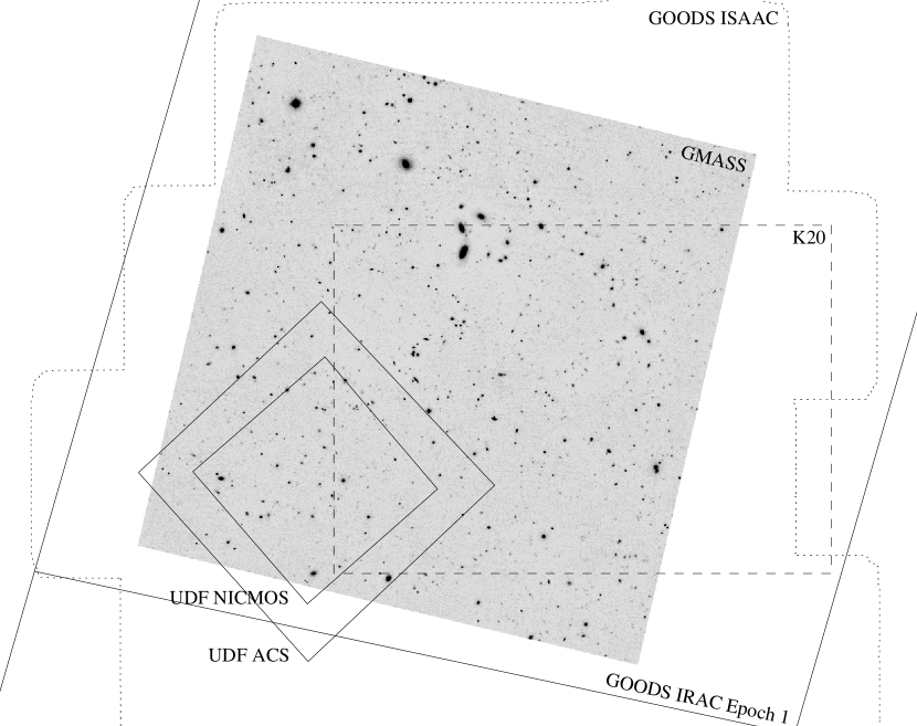
Figure 1: Location of the GMASS field (greyscale, $K_{s}$ band) compared to other fields (K20, dashed) and instrument imaging (UDF NICMOS and ACS, diamonds; GOODS ISAAC, dotted; GOODS IRAC, large rectangular, with Epoch 1 indicated) coverages. The GMASS field was chosen to be inside the IRAC Epoch 1 and ISAAC imaging, covering as much as possible of the UDF and K20 field. North is up, east to the left.

The GMASS sample was constrained to objects detected within a square field of $6\aas@@fstack{\prime}8\times 6\aas@@fstack{\prime}8$, centred at R.A. = 3^h32^m31^s3 and DEC = -27^∘46′07 (J2000) and with position angle -13.2^∘ (north to east, see Fig. 1). The field geometry is equal to that of the 46.2 square arcmin field of view of the FORS2 instrument and contains enough spectroscopic targets to fill the six masks designed for the GMASS spectroscopic survey. It was chosen to be completely within the area covered by the IRAC observations of CDFS, but at the same time cover as much of the Hubble Ultra Deep Field (UDF) and K20 field (Cimatti et al. 2002b) as possible.

2.3 IRAC observations and photometry

As the main contributors to the light of massive galaxies are, even at high redshift, old stars that emit most of their light at wavelengths above 4000 Å, it is important to analyse this red light when estimating the mass of a galaxy. This is illustrated by the properties of the galaxies found by the successful Lyman-break technique, which identifies high redshift galaxies based on their strong emission in the rest-frame UV and therefore selects almost exclusively young, low-mass, strongly star-forming galaxies (Steidel et al. 2003). The red, more massive, and (relatively) less active distant galaxies are more difficult to find, but progress also has been made here, for example using the $BzK$ selection technique (Daddi et al. 2004). However, to select distant galaxies mainly on the basis of mass, radiation redward of one micron in the rest-frame needs to be detected, as variations in the mass-to-light ratio with stellar population age are smaller at longer wavelengths, where longer-lived, cooler stars contribute a larger fraction of the integrated luminosity. This became possible with the launch of the Spitzer Space Telescope, which is equipped with a sensitive MIR camera (IRAC).

IRAC is a four-channel camera that provided (at the time of cryogenic operation) simultaneous 5$\aas@@fstack{\prime}$2$\times$5$\aas@@fstack{\prime}$2 images at 3.6, 4.5, 5.8, and 8.0 microns (Fazio et al. 2004). The spatial resolution of the IRAC images is limited primarily by the telescope itself, i.e. by its aperture of 85 cm, resulting in a point spread function (PSF) full width at half maximum (FWHM) of $\sim$1.6″ at 4.5 microns.

The IRAC CDFS observations were obtained as part of the Great Observatories Origins Deep Survey (GOODS) Spitzer campaign and targeted at R.A. = 3^h32^m30^s37 and DEC = -27^∘48′16$\aas@@fstack{\prime\prime}$8 (J2000) with a mean position angle of -14 degrees. The exposure time per channel is approximately 23 hours. The data was reduced by the (Spitzer) GOODS team and have magnitude limits at signal-to-noise ratios (S/N) of 5 for point sources corresponding to m_AB=26.1, 25.5, 23.5, and 23.4 at 3.6, 4.5, 5.8, and 8.0 microns (Dahlen et al. 2010).

For the first version of our catalogue, only the first epoch of IRAC observations of GOODS-S were available, in which the GMASS area was covered by data at 4.5 and 8.0 $\mu$m. Sources were detected in the 4.5 $\mu$m channel with SExtractor (Bertin & Arnouts 1996), using a Gaussian detection kernel. After careful inspection of blended and unblended sources, we found that the projected distance between sources detected in IRAC images and their counterparts in the $K$ band indicates whether a source is blended in the IRAC image. Empirically, we found that the criterion of $<$ 0$\aas@@fstack{\prime\prime}$5 separation, applied by ourselves, is efficient at discarding the vast majority of substantially blended sources. It was found that approximately 25% of the sources to the m(4.5) $<$ 23.0 limit were blended. After the second epoch of IRAC observations, data at 3.6 and 5.8 $\mu$m covering the GMASS area became available. A new catalogue was generated of sources detected in a summed image of channel one and two, after applying a Mexican hat kernel. The higher deblending efficiency of this kernel resulted in only $\sim 10$% of the sources being blended (see also Daddi et al. 2007b). Monte Carlo simulations were performed by the GOODS Team (in particular H. Ferguson), by placing point sources at random in the IRAC images and using an empirical PSF created by the Spitzer Science Center. The simulations confirm the empirical conclusion because about 10% of the simulated galaxies were detected further than 0$\aas@@fstack{\prime\prime}$5 from their original position, at $m(4.5)=23.0$, for the Mexican hat kernel (and a significantly larger fraction for the Gaussian kernel). The simulations also show that for sources unresolved at the IRAC resolution (such as distant galaxies), we recover about 90% of the simulated sources at $m(4.5)=23.0$.

Galaxy photometry in the IRAC bands was performed using 4″ diameter apertures. Monte Carlo simulations were developed to measure photometric aperture corrections to total magnitudes. The resulting aperture corrections were 0.316, 0.355, 0.548, and 0.681 magnitudes for the four IRAC channels.

The GMASS sample was extracted from the public IRAC 4.5 $\mu$m image of GOODS-South adopting a limiting magnitude of $m(4.5)\leq 23.0$ (AB system), corresponding to a limiting flux of 2.3 $\mu$Jy. In this respect, the GMASS sample is a pure flux–limited sample with no additional colour selection criteria. The choices of 4.5$\mu$m band and the cut of $m(4.5)\leq 23.0$ are the result of several considerations related to the scientific aim of the project, the survey design, and the spectroscopic multiplexing. The main reasons can be summarised as follows:

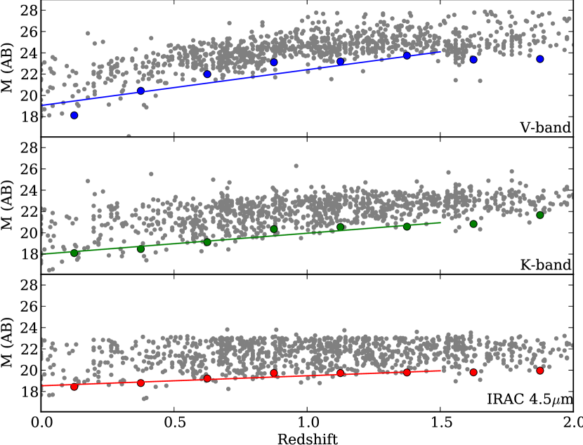
Figure 2: Magnitudes as a function of photometric redshift for the GMASS sample, in the ACS F606W band (top), ISAAC K_s band (middle), and IRAC 4.5 $\mu$m (bottom). A straight line is fit to the median of the brightest 5% in each $\Delta$z=0.25 bin, up to $z$=1.5, that has a slope of 3.4, 2.0, and 0.9, respectively. This shows the relative strength of the K-correction for these bands, which is strong in $V$-band, and much weaker in the infrared IRAC band.

(1) At the time the initial GMASS catalogue was developed, only the 4.5 and 8 $\mu$m images were available for the CDFS field. A severe problem that occurs with this type of data is the blending of sources due to the combination of low spatial resolution and high sensitivity. The background confusion limit is therefore relatively quickly reached in channel four, while the 4.5$\mu$m band is the optimal compromise among the IRAC bands in terms of sensitivity, PSF, and image quality, and has minor blending problems. Moreover, it samples the rest-frame near-infrared up to $z\sim 3$ (i.e. the expected upper redshift envelope of the GMASS sample), thus allowing a selection that is most sensitive to stellar mass. In addition, the 4.5$\mu$m band detects the redshifted rest-frame 1.6 $\mu$m peak of the stellar SEDs for $z>1.5$, which is consistent with the cut applied to photometric redshifts. The gradual shift of the 1.6 $\mu$m peak in the 4.5 $\mu$m band for $z>1.5$ is also responsible for a negative k–correction effect, as illustrated in Fig. 2, similar to that occurring in the submillimetre for dusty galaxies (Blain & Longair 1993).

(2) The limiting flux of $m(4.5)\leq 23.0$ was dictated partly by the observational constraints imposed by the FORS2 mask exchange unit (MXU) multiplexing, i.e. by the number of available slits with respect to the surface density of targets at $z>1.4$ available in the field. We carried out several tests by varying the limiting magnitude, extracting the corresponding samples of galaxies with $z>1.4$, and checking whether an appropriate number of targets was available to maximise the number of targets and slits for both the blue and red grism spectroscopy. The cut $m(4.5)\leq 23.0$ represented the best compromise.

(3) The photometric completeness at $m(4.5)\leq 23.0$ is 90%.

(4) At magnitudes fainter than $m(4.5)=23.0$, the fraction of objects affected by blending increases significantly (e.g., from 10% at $m(4.5)=23.0$ to 50% at $m(4.5)=25.0$).

(5) At $m(4.5)\leq 23.0$, the selection is sensitive to stellar masses down to $\log(M/M_{\odot})\approx 10.5$ for all redshifts ($0<z<3$), using a Chabrier initial mass function (IMF). In particular, the limiting mass sensitivities are $\log$(M/M${}_{\odot})\approx$ 9.8, 10.1, and 10.5 for $z=1.4$, 2, and 3, respectively. This ensures that it is possible to investigate the evolution of the galaxy mass assembly within a mass range extending from the possible precursors of massive galaxies (e.g., individual galaxies with $\log(M/M_{\odot})\approx 10$ that merge to form a more massive system) to the most massive objects available at $z>1.5$.

2.4 Optical and NIR observations and photometry

Our optical and NIR data set consists of publicly available images provided by several institutes. The ground–based data includes observations in the $U^{\prime}$, $U$, $B$, $V$, $R$, $I$, $J$, $H$, and $Ks$ bands, some provided by ESO as part of its participation in the GOODS project.

The $U^{\prime}$ and $U$ band observations (PI J. Krautter) were conducted at the ESO/MPG 2.2 m telescope at La Silla using the Wide-Field Imager (WFI, Baade et al. 1999). The data, which cover the full CDFS field, have a seeing of 1$\aas@@fstack{\prime\prime}$1 and 1$\aas@@fstack{\prime\prime}$0 and reach a 5$\sigma$ limiting magnitude, as measured within a 2 $\times$ FWHM aperture, of 26.0 and 25.7 for $U^{\prime}$ and $U$, respectively (Arnouts et al. 2001). We used release DPS_2.0 (7 Mar 2001), which had been reduced by the ESO Imaging Survey (EIS, Renzini & da Costa 1997) Team. Deeper $U$ and $R$ band data obtained with the VIsible Multi-Object Spectrograph (VIMOS, LeFevre et al. 2003) at the VLT became available after we had constructed our catalogue (Nonino et al. 2009).

The $B$, $V$, $R$, and $I$ band observations were conducted at the ESO/VLT 8.2 m telescope, using FORS1. The images have a seeing of $\sim$0$\aas@@fstack{\prime\prime}$7 and cover only part of the GMASS field, their top edge being at DEC = -27^∘42′45$\aas@@fstack{\prime\prime}$49 (J2000). For a description of the data, we refer to Giacconi et al. (2001), Rosati et al. (2002), and Szokoly et al. (2004).

The $J$, $H$, and $K_{s}$ band observations were conducted at the ESO/VLT 8.2 m telescope, using the Infrared Spectrometer And Array Camera (ISAAC, Moorwood et al. 1998). At the time the GMASS catalogue was constructed, only the $J$ and $K_{s}$ bands were available (GOODS/EIS release v1.0, 30 April 2004). The $H$ band (from release v1.5, 30 September 2005) data were later added, but not used for the photometric redshift determination described in Sec. 2.6. The individual ISAAC pointings are assembled to form a mosaic covering the entire GMASS field (and more). The seeing in the individual tiles varies from 0$\aas@@fstack{\prime\prime}$4 to 0$\aas@@fstack{\prime\prime}$6, and the 1$\sigma$ sky background limit in a circular aperture of 0$\aas@@fstack{\prime\prime}$7 diameter from 27.4 to 27.8, from 26.6 to 27.4, and from 26.6 to 27.2, for $J$, $H$, and $K_{s}$ bands, respectively (Retzlaff et al. 2010).

The space–based data includes optical observations taken with the Advanced Camera for Surveys (ACS) and NIR observations taken with the Near Infrared Camera and Multi Object Spectrometer (NICMOS), both aboard the Hubble Space Telescope (HST). The GOODS ACS images (Giavalisco et al. 2004) were taken with the Wide Field Channel (WFC), in four broad, non-overlapping filters: F435W ($B_{435}$), F606W ($V_{606}$), F775W ($i_{775}$), and F850LP ($z_{850}$) with exposure times of 3, 2.5, 2.5, and 5 orbits per filter, respectively. The resulting 10$\sigma$ point-source sensitivities within an aperture diameter of 0$\aas@@fstack{\prime\prime}$2 are 27.8, 27.8, 27.1, and 26.6, respectively. The values reported are medians over the area covered by the HST/ACS imaging. We used the images reduced by the GOODS team, which was released as version 1.0 (29 August 2003). The Ultra Deep Field (UDF) is located partly within the GMASS field. The ACS UDF observations consist of a single pointing at R.A. = 3^h32^m39^s0 and DEC = -27^∘47′29$\aas@@fstack{\prime\prime}$1 (J2000) imaged through the same four ACS filters as used in GOODS but for a longer time, i.e. for 56, 56, 144, and 144 orbits, respectively. The expected 10$\sigma$ limiting magnitudes in an aperture of 0.2 square arcsec are 28.7, 29.0, 29.0, and 28.4, respectively. The UDF is also (almost completely) covered by a 3$\times$3 mosaic of NICMOS pointings through the two broad–band filters F110W ($Y_{110}$) and F160W ($H_{160}$), each filter being exposed during 8 orbits. This resulted in a 5$\sigma$ S/N of magnitude 27.7 through a 0$\aas@@fstack{\prime\prime}$6 diameter aperture at both 1.1 and 1.6 $\mu$m (Thompson et al. 2005). We used the ACS and NICMOS data released as version 1.0 (9 March 2004). We note that the CDFS field will also be covered by the Cosmic Assembly Near-IR Deep Extragalactic Legacy Survey (CANDELS), using the Wide Field Camera 3 on HST (Koekemoer et al. 2011; Grogin et al. 2011), providing much more sensitive NIR images than the NICMOS images used by us, and covering all of the GMASS field.

We decided to use the $K_{s}$ image as the basis of our multi-band image stack, that is, we cropped the $K_{s}$ image to produce the smallest size image that still encompassed the GMASS field (whose orientation is not such that north is up). Since the $J$ and $H$ band images have the same pixel scale, we performed the same procedure, after matching their positions to the $K_{s}$ band image using the accurate astrometry from the header. The other images have different pixel scales and were therefore transformed to match the geometry of the $K_{s}$ band image using at least 200 detected objects per image, except for the smaller NICMOS mosaic where 162 objects were used, and the shallower $U^{\prime}$ and $U$ band images, where 75 objects were used. The RMS deviations resulting from a surface fit to the matched object data were about 0$\aas@@fstack{\prime\prime}$08 for the HST images, 0$\aas@@fstack{\prime\prime}$2 for the $U^{\prime}$, $U$ band WFI images, 0$\aas@@fstack{\prime\prime}$04 for the $V$, $I$ band images, and 0$\aas@@fstack{\prime\prime}$1 for the $B$, $R$ images. The same procedures were followed for the associated weight maps.

Subsequently, SExtractor (Bertin & Arnouts 1996) was used in two-image mode repeatedly on all images and their associated weight maps to carry out matched-aperture photometry, using the $K_{s}$ image as a detection image. For the photometry, 1$\aas@@fstack{\prime\prime}$5 diameter circular apertures were used. The transformation of the images described above causes the noise to be correlated between the pixels. SExtractor, however, assumes the noise to be uncorrelated between pixels for its noise computation. We therefore corrected the noise output from SExtractor by a factor determined from independent noise measurements with IRAF. This factor depends on the band but was typically below 2.0. Objects had to have five contiguous pixels with a S/N of $>$$1.5\sigma$ to be detected, resulting in 2609 $>$$3.3\sigma$ detections, the faintest having $K_{s}$ = 25.8. We also created a multi-band catalogue with objects that have five contiguous pixels with a S/N of $>$$1.0\sigma$, resulting in 6207 $>$$2.2\sigma$ detections, the faintest having $K_{s}$ = 26.6, where faintest is in this case defined as having an error in their magnitude smaller than 0.1. We call this the faint catalogue. This catalogue was only used to find four counterparts to IRAC detections not present in the main $K_{s}$ based catalogue (see Sec. 2.5).

We determined absolute magnitudes by applying a correction to each band separately. The correction per band was determined by comparing the circular aperture magnitudes with SExtractor’s BEST magnitude (the Kron magnitudes for unblended cases and the isophotal one for blended cases), for those objects deemed to be unresolved (i.e. SExtractor’s stellarity $>$ 0.90 and S/N $>10$). The correction factors correlate quite well with the seeing on the images, i.e. the ACS images have corrections in the range 0.03–0.04, the NICMOS images 0.06–0.08, the ISAAC images 0.11–0.13, the FORS images 0.18–0.24, and the WFI images 0.37–0.40.

As object detection was performed twice, once in the $K_{s}$ band and once in the 4.5$\mu$m band, it is useful to know the completeness of the $K_{s}$ band catalogue obtained. We therefore compared the number counts of the $K_{s}$ band catalogue and the faint $K_{s}$ band catalogue with literature number counts obtained from Gardner et al. (1993) and Saracco et al. (2001). As shown in Fig. 3, the number counts (up to $K_{\rm Vega}=22.5$) from our catalogue agree well with the literature counts. The number of sources detected in the $K_{s}$ band catalogue deviates significantly and abruptly from the faint catalogue at $K_{\rm Vega}>22.0$ (or $K_{\rm AB}>24.0$), which we therefore accept as the completeness limit.

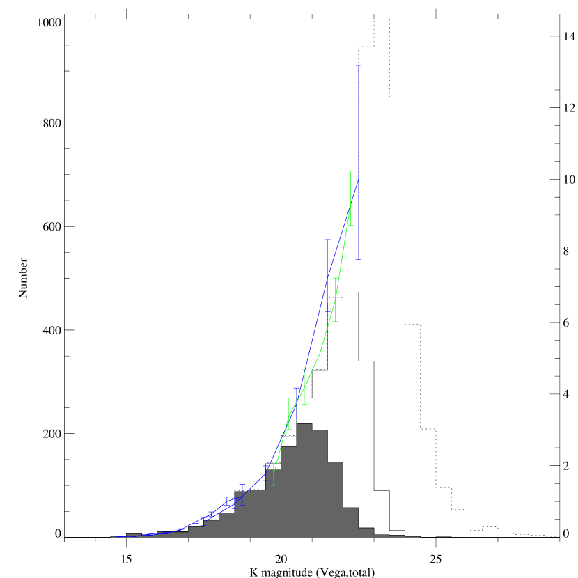
Figure 3: $K$ band counts for the 49.75 arcmin² GMASS field. Also indicated on the right-hand axis are counts/mag/arcmin². The solid histogram is for the 3.3$\sigma$ $K$ band catalogue, while the dashed histogram is for the (faint) 2.2$\sigma$ catalogue. The filled histogram indicated which objects are in the GMASS catalogue (i.e., are counterparts of an unblended 4.5 $\mu$m source). The vertical dashed line indicated the completeness limit for the 3.3$\sigma$ catalogue. Overplotted are counts from Gardner et al. (1993, green/light line) and Saracco et al. (2001, blue/dark line).

2.5 Combination of IRAC and optical-NIR catalogues

To construct the final multi-band catalogue, i.e., the GMASS catalogue, covering wavelengths from the UV to the MIR, the optical-NIR catalogue and the IRAC catalogue were combined by matching both catalogues. This matching was done by searching for counterparts to the IRAC 4.5 $\mu$m detections in the $K_{s}$ band catalogue at a distance of $\leq$ 1″ or less, using the centroid celestial coordinates. Since the spatial resolution of the IRAC channel 2 image is not as good as that of the $K_{s}$ band, some IRAC detections have two or even three possible NIR counterparts. All multiple counterpart cases were checked by eye and if an unambiguous counterpart could be allocated by eye, it was added to the GMASS catalogue. In some cases, only a likely counterpart could be identified, which was also added to the catalogue but flagged as ambiguous. At the time when only the first IRAC catalogue was available (epoch 1, channels 2 and 4), this process resulted in a list of 1202 objects, from which the spectroscopic sample was selected. We later repeated the process, using the second IRAC catalogue (epoch 1+2, all channels), adding 70 new objects.

For almost all IRAC sources, we found counterparts in the main $K_{s}$ based catalogue. To find the remaining missing optical-NIR counterparts, we checked the faint $K_{s}$ based catalogue and added four objects from this catalogue. Two, apparently very red, 4.5 $\mu$m detections remained completely without a counterpart and were added to the GMASS catalogue without optical-NIR information. We note that 52 of the original 1202 4.5 $\mu$m detections are not present in the second IRAC catalogue but were retained in the GMASS catalogue as two had already been included in the first two GMASS spectroscopy masks. These were mostly faint sources that, although just being below the cut-off magnitude in the original catalogue ($m(4.5)\leq 23.0$), had a magnitude just above the cut-off in the second IRAC catalogue. In addition, some sources that were within the 1″search radius in the original catalogue had moved outside this radius in the second. Four bright sources were not present in the second catalogue as they were either blended with other nearby sources or close to a region containing artifacts from a bright star. After we determined spectroscopic redshifts, we added 28 more objects to the catalogue. These were included in the masks as fillers or serendipitously. The final GMASS catalogue contains 1305 objects.

The internal consistency of the photometry in the GMASS catalogue was tested by comparing optical, NIR, and IR photometry of stars in the field using models by Lejeune et al. (1997) and Bruzual & Charlot (2003), and IRAC observations by Eisenhardt et al. (2004). As some discrepancy with the IRAC photometry could not be ruled out to better than 10%, we added this uncertainty in quadrature to the measurement errors in the IRAC photometry.

Only 7% of the sources in the GMASS catalogue have magnitudes fainter than $K_{\rm Vega}=22.0$, where the $K_{s}$ band catalogue is incomplete. The number of 4.5$\mu$m counterparts in the $K_{s}$ band begins to deviate slightly from the total number of $K_{s}$ band counts at $K_{\rm Vega}=19.5$ and significantly at $K_{\rm Vega}=20.5$, indicating that many $K_{s}$ band sources fainter than this limit do not have an IRAC counterpart with $\rm m_{4.5\mu m}<23.0$, either because these counterparts are indeed fainter than $\rm m_{4.5\mu m}=23.0$ or these counterparts are blended with other sources in the IRAC image.

Within the catalogue, there are several objects that have been found in other papers to be peculiar. Using the deep ACS and NICMOS images in the UDF, Chen & Marzke (2004) identified nine galaxies at (their) photometric redshift $z>2.8$ that exhibit a pronounced discontinuity between the F110W and F160W bandpasses. These discontinuities are consistent with redshifted 4000 Å breaks in E/S0 and Sab galaxy model templates. After some additional analysis of these nine galaxies, they concluded that five of them have stellar masses comparable to the present-day M_∗ and are at least 1.6 Gyr old. Yan et al. (2004) used the same data in addition to IRAC observations, to select objects with $f_{\nu}(3.6\mu m)/f_{\nu}(z_{850})>20$, called IEROs for IRAC-selected extremely red objects. After discarding 58 objects, whose IRAC photometry may be inaccurate because of nearby objects, they retain a sample of seventeen bona-fide IEROs. The SEDs of these objects are best explained by the presence of an old ($\sim$1.5–2.5 Gyr) stellar population in galaxies at $1.6<z<2.9$ with stellar masses of 0.1–1.6 $\times 10^{11}$ M_⊙. All nine objects from Chen & Marzke and 14 objects from Yan et al. are included in the GMASS catalogue. Four of these are common between the two papers.

2.6 Photometric redshift determination

Photometric redshifts for the objects in the GMASS catalogue were estimated by applying the HyperZ software, version 1.1 (Bolzonella et al. 2000). This photometric redshift code is based on the fitting of given spectral energy distributions (SEDs) to the observed data. Using a range of redshifts and reddening vectors, the sum of the squared difference between the observed and template flux divided by their uncertainty, is minimised. Redshifts were computed between $z=0$ and $z=5$ in steps of $\Delta z=0.044$. A range of reddening was also applied, using Calzetti’s reddening law (Calzetti et al. 2000) with $A_{V}$ between 0 and 1 magnitude and steps of 0.1 magnitude. These parameter ranges are very broad and we therefore assume they represent flat priors.

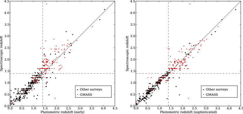
Figure 4: Plots of spectroscopic versus photometric redshifts for 309 galaxies in the GMASS field with secure redshifts determined in other surveys (dark [black] circles) and 160 galaxies with secure redshifts determined by GMASS spectroscopy (bright [red] squares). The latter set of redshifts are shown here only to illustrate the quality of the photometric redshifts. They were not used to optimise the photometric redshifts itself. The plot on the left shows the early photometric redshifts used to select the spectroscopic sample (based on the partly available IRAC images available at that time), while the plot on the right shows the photometric redshifts determined later, using all four IRAC bands, but based on the same set of 309 spectroscopic redshifts.

The resulting photometric redshifts were compared to 309 secure spectroscopic redshift values in the GMASS field available from the literature (at that time, see Sec. 2.7). Assessing the difference between the fitted template flux and the observed flux for all objects in the catalogue revealed systematic offsets for some bands, which indicates that the colour terms are caused mainly by the incorrect relative flux-calibration between the bands, at least for the aperture photometry used here. After correcting these offsets, the photometric code was run again to see whether photometric redshifts closer to the known spectroscopic redshifts could be obtained, at which point the last two steps could be repeated again, a process called tuning. We performed a large number of tuning steps, which also involved including different template spectra and excluding some observing bands (as some ground-based bands overlap with some space-based bands). After 28 runs, we concluded that we had obtained optimal results, given the data at hand. The tuning resulted in zero-point offsets of -0.35,-0.33 for the U’ and U bands, and values between -0.15 and 0.19 for the other bands, except for the offsets for the IRAC 3.5 and 4.5 $\mu$m bands, which were 0.18 and -0.21, respectively. These offsets most likely represent corrections needed for imperfect PSF matching, and possibly by partly inadequate template SEDs. The zero-point offsets were only applied to the photometric catalogue used as input for the determination of photometric redshifts, not to the catalogue used to construct plots in the remainder of the paper. The mean difference divided by $(1+z)$ and its standard deviation (RMS) between these photometric redshifts and 309 secure redshifts from the literature were $\Delta(z)=-0.0002$ and $\sigma(\Delta(z))=0.014$. The final SED of templates used consisted of four empirical templates and two model templates. The empirical templates, which were provided with the HyperZ software, were constructed by taking the mean spectra of local galaxies from Coleman et al. (CWW SEDs, 1980) and extending these to both the UV and IR regions using Bruzual & Charlot models (BC93, Bruzual A. & Charlot 1993) with parameters (SFR and age) selected to match the observed spectra (Bolzonella et al. 2000). These four templates represent average E/S0, Sbc, Scd, and Im galaxies, but cannot reproduce the very blue SEDs found for some high redshift galaxies. To alleviate this problem, two model SEDs were added, representing very young galaxies of 100 Myr and 1 Gyr old, generated with the BC03 spectral synthesis code. As the ISAAC $H$ band and the IRAC channel 1 and 3 bands were unavailable at the time we estimated the photometric redshifts, they were not used in this run. In addition, the FORS $I$ band was excluded because it is shallower than the other available $I$ bands. For the $B$ band, the UDF ACS band was used if available, or otherwise the FORS $B$ band, and in places where neither of those were available the GOODS ACS band. The optical/NIR magnitudes were boosted per object to match the IRAC magnitudes, by the difference between SExtractor’s BEST magnitude and the corrected aperture magnitude in the $K_{s}$ band for that object. We checked by eye the observed SEDs and the fits made by HyperZ for objects with $z_{\rm phot}>2.5$, all of which seemed to be fine.

After the selection of targets for spectroscopy, imaging data of the CDFS for all four IRAC bands became available, and a more sophisticated photometric-redshift determination was then attempted, resulting in $\Delta(z)=0.013$ and $\sigma(\Delta(z))=0.010$. These later set of redshifts are used in the analyses in this publication. In Fig. 4, we plot the photometric versus spectroscopic redshifts for the 309 galaxies with known spectroscopic redshifts, for both the early photometric-redshift determination and the later, more sophisticated, determination. We also plot the redshifts determined by GMASS, which illustrate that the scatter at high redshifts (where few redshifts were formerly known) is smaller for the second set of photometric redshifts.

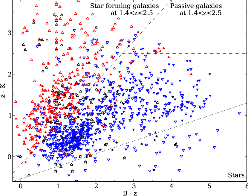
Figure 5: $B-z$ vs $z-K$ plot of all GMASS objects. Closed symbols represent objects with secure spectroscopic redshifts. For the remaining (open) symbols, the photometric redshift is used. Upward pointing triangles indicate $z>1.4$; these are grey [red] for the range $1.4<z\leq 2.5$ and black for $z>2.5$. Downward pointing (blue) triangles $z\leq 1.4$ and (black) stars indicate $z=0$ (i.e., stars). No special effort has been undertaken to identify stars based on their spatial appearance, hence most downward pointing symbols in the stellar region will indeed be stars. The limits of the $BzK$ selection are indicated by dashed lines.

Apart from photometric redshifts based on many photometric bands, certain colour-colour selections can also give a good indication of the redshift for particular redshift intervals. A colour-colour selection of special interest to our purposes, i.e. the selection of galaxies at $z>1.4$, is the $BzK$ selection (Daddi et al. 2004). Applying the criterion $BzK=(z-K)-(B-z)>-0.2$ allows us to select actively star-forming galaxies at $1.4\la z\la 2.5$, independent of their dust reddening, while objects with $BzK<-0.2$ and $(z-K)>2.5$ colours include passively evolving galaxies in the same redshift range. A plot (see Fig. 5) of the $B-z$ and $z-K$ colours of the objects in the GMASS catalogue, with the colour selection superimposed, shows that the photometric redshifts and the $BzK$ selection method are indeed consistent. Of the 1275 objects with photometric redshifts, 429 have $z_{\rm phot}>1.4$ and 865 $z_{\rm phot}\leq 1.4$. Of the former (latter), 349 (92) fall in the region allocated to $z>1.4$ by the BzK method. The $BzK$ selection method, however, should be most effective for the selection of galaxies at $1.4<z<2.5$ (Daddi et al. 2004). The number of objects with $1.4<z_{\rm phot}\leq 1.4$ is 343, while 934 have $z_{\rm phot}\leq 1.4$ or $z_{\rm phot}>2.5$. Of the former (latter), 303 (138) fall in the region allocated to $1.4\la z\la 2.5$ by the BzK method. On the basis of photometric redshifts, the $BzK$ selection seems therefore to select $1.4<z<2.5$ galaxies with an efficiency of 69% and to suffer 21% contamination by $z<1.4$ galaxies.

2.7 Other spectroscopic surveys in the CDFS field

In addition to deep imaging, the CDFS field has extensive optical spectroscopic coverage. In particular, ESO has carried out spectroscopic observations of all galaxies in both GOODS fields down to a magnitude of 24–25, with this limiting magnitude being in the $B$ and $V$ bands for objects observed with VIMOS and in the $z$ band for objects targeted with FORS2, both mounted at the VLT. At the time that the GMASS spectroscopic sample was defined, Vanzella et al. (2005, 2006) reported that the first two FORS2 releases together contained 930 observed sources and 724 redshift determinations. They used five categories of target selection, one of which (partly) overlaps with the GMASS selection, namely, the photometric–redshift selection based on the redshifts determined by Mobasher et al. (2004) of galaxies at $1<z_{\rm phot}<2$. We note, however, that the GMASS target selection also includes significantly fainter objects. The full dataset of the ESO/GOODS FORS2 campaign was presented by Vanzella et al. (2008) and contains a total of 887 redshift determinations (obtained from 1715 spectra of 1225 individual targets). In addition, spectroscopic identifications for 114 additional galaxies were obtained in this field by Vanzella et al. (2009). These, however, are $B$, $V$, and $i$-band dropouts, at mean redshifts $z\sim 4$, 5, and 6. The VIMOS spectroscopy in the CDFS is part of the larger VIMOS VLT Deep Survey (VVDS, Le Fevre et al. 1998) and targets galaxies as faint as $I\sim 24$. At the time of the GMASS spectroscopic sample definition, Le Fèvre et al. (2004) reported that 784 redshifts were determined within the GOODS field. The redshift distribution was peaked at a median redshift $z=0.73$, but also contained some redshifts at $z>1.4$, up to $z\sim 4$. The full GOODS/VIMOS spectroscopic campaign (Popesso et al. 2009; Balestra et al. 2010) produced 3218 redshifts, obtained from 5052 spectra. These were observed with either the blue or orange grism, targeting galaxies at $1.8<z<3.5$, and $z<1\cap z>3.5$, respectively. Another large VIMOS survey, aimed at intermediate mass galaxies at $z\leq 1$ by Ravikumar et al. (2007), provided an additional 531 redshifts in the CDFS.

The optical counterparts of X-ray sources found by Chandra in the CDFS were observed by Szokoly et al. (2004), who presented spectroscopic redshifts for 168 sources, mostly with magnitudes $R<24$. Another, smaller, quasi-stellar object (QSO) survey based on optical and NIR photometry was carried out by Croom et al. (2001), resulting in 14 measured redshifts. In addition, the K20 survey was carried out in the CDFS (Cimatti et al. 2002a). This survey was designed to obtain optical and NIR spectral information and redshifts of a complete sample of 545 objects to $K_{s,{\rm Vega}}\leq 20.0$ over two independent fields, one of which is the CDFS. The reported redshift identification completeness is very high ($>92$%, and has been increased to an even higher percentage by the current work, see Sec. 6.4).

During our target selection, we excluded all the targets with secure redshifts that were known at the time that the GMASS spectroscopic sample was defined and available from the surveys mentioned above. At the time of the GMASS spectroscopic target selection, not all of the above surveys had been finished. In these cases, we avoided all galaxies targeted by these surveys, as derived from the target lists provided to us by the authors (e.g., Vanzella et al., private communication). In addition, we excluded the 29 distant supernova (SN) host galaxies with secure spectroscopic redshifts found by Strolger et al. (2004) in the CDFS. The redshifts known in the CDFS were collected by Balestra et al. (2010) in a master catalogue that we extend with those obtained in the GMASS survey.

2.8 Selection of targets for ultra-deep spectroscopy

The goal of our spectroscopic campaign was to study a mass-selected sample of galaxies at high redshift. The mass selection is taken care of by the use of IRAC photometry ($\rm m_{4.5\mu m}\leq 23.0$), while the high redshift selection is guaranteed by the photometric redshift estimates ($z_{\rm phot}\geq 1.4$). We did not select sources on the basis of their observed magnitudes, but we did set magnitude limits to assure that spectroscopy was possible, of $I\leq 26.0$ and $B\leq 26.0$ for the red and blue masks, respectively. For P74, the $B$ band limit was set to $B\leq 26.5$ because we had seen from a first assessment of the blue P73 mask that the S/N of the faintest objects in the mask was still sufficient. In addition, we divided the selected objects into two samples: those most suitable for inclusion in the red masks being red and at intermediate redshift, such that $z-K_{s}\geq 2.3$, $z_{\rm phot}\leq 2.5$ and those most suitable for inclusion in the blue masks, being blue with $z-K_{s}<2.3$ or having $z_{\rm phot}>2.5$ such that UV absorption lines are redshifted in the optical domain.

The target selection was done separately for P73 and, after a first assessment of the results of P73, for P74. For P73, using the constraints given above, 128 and 32 objects were selected for inclusion in the blue and red masks, respectively. After a visual assessment of the IRAC detections, some objects were removed from this selection, as they seemed to have inaccurate photometry because of blending (they were near bright objects), leaving 122 and 30 objects in the blue and red parts of the spectroscopic target list, respectively.

For P74, we excluded objects that already had been targeted in the P73 masks. For the blue masks, we found 95 targets, using the fainter $B$ band limit. This would have been 146, if the objects in the P73 masks had not been excluded. For the red mask, we used some extra constraints to set priorities. As highest priority targets (16), we selected objects in the upper left part of the BzK diagram, i.e. with $BzK<-0.2$ and $z-K>2.5$, in the upper right, i.e. with $BzK>-0.2$ and $z-K>2.7$, objects with $z_{\rm phot}>4.0$, and HyEROs, i.e. with $J-K>3$ (Vega magnitudes). As second priority objects (25), we selected galaxies that had not already been included in the steps above, which are faint in blue, but not bright enough in red, i.e. $B>26.5$. As third priority objects (18), we selected objects that had already been included in the red P73 mask, but were very faint and/or not observed through optimal slits, and objects close to the upper left part of the BzK diagram, i.e. $BzK<-0.2$ and $2.2<z-K<2.5$, without selecting on the basis of photometric redshift.

An additional 24 objects would have satisfied the constraint for inclusion in the spectroscopic target list, had they not already secure spectroscopic redshifts obtained in other surveys.

Table 1: Spectroscopic sample selection criteria and redshift determination statistics

				Selection criteriaa			Targets actually observed					$z_{\rm spec}$$\geq$0		$z_{\rm spec}$$>$1.4
ID	Pb	Prioc	M(AB)d	$z_{\rm phot}$	other	#	Tote	Redf	Bluef	P73g	P74g	q=1h	q=0h	q=1h	q=0h
S2	P73	B1	B$<$26.0	1.4$<$$z$$<$2.5	$z$$-$K$<$2.3	122	103	31	91	39	71	95	4	90	4
S5b	P73	B2	B$<$26.0	$z$$>$2.5		5	5	1	5	5	2	5	0	5	0
S1	P73	R1	I$<$26.0	1.4$<$$z$$<$2.5	$z$$-$K$>$2.3	30	24	23	2	17	12	12	4	12	3
S5	P73	R2	I$<$26.0	$z$$>$2.5		23	15	10	7	5	12	7	3	6	3
S6	P73	R3	I$<$26.0	1.4$<$$z$$<$2.5	1.8$<$$z$$-$K$<$2.3	22	15	13	4	6	11	9	2	9	2
S7	P73	R4	I$<$26.0	1.4$<$$z$$<$2.5	1.6$<$$z$$-$K$<$1.8	18	15	8	9	9	8	10	3	10	3
S8	P73	R5	I$<$26.0	1.4$<$$z$$<$2.5	1.4$<$$z$$-$K$<$1.6	24	17	7	12	7	14	13	0	12	0
	P73	Total unique targets in P73 samples (S2-S8)				202	86	61	34	44	57	51	12	49	11
S21	P74	B1	B$<$26.5	$z$$>$1.4	$I$$>$26.0	1	1	1	1	0	1	1	0	1	0
S22	P74	B2	B$<$26.5	$z$$>$1.4	$I$$<$26.0	94	71	19	70	1	70	64	2	59	2
S25	P74	R1	I$<$26.0	-	$B$$z$$K^{\mathrm{i}}$, $z$$-$$K$$>$2.5	8	8	8	0	0	8	7	1	5	0
S27	P74	R2	I$<$26.0	$z$$>$4.0		4	4	4	0	0	4	1	2	0	2
S28	P74	R3	I$<$26.0	$z$$>$1.4	$B$$<$26.5	25	12	12	0	0	12	5	3	5	3
S29	P74	R4	I$<$26.0	-	$B$$z$$K^{\mathrm{i}}$, 2.2$<$$z$$-$$K$$<$2.5	11	9	9	0	0	9	7	0	1	0
S30	P74	R5	I$<$26.0	-	$J$$-$$K$$>$3 (Vega)	3	3	3	0	0	3	0	1	0	1
S31	P74	R6	Promising faint targets in P73 masks			7	7	7	0	7	6	3	1	3	1
	P74	Total unique targets in P74 samples (S21-S31)				144	114	62	71	8	112	88	10	74	9
P73+P74		Total unique targets in red or blue sample				221	174	92	105	66	125	135	15	120	13
P73+P74		Total unique targets in red sample				135	102	77	34	44	73	64	14	54	12
P73+P74		Total unique targets in blue sample				140	115	34	103	44	80	104	4	98	4
P73+P74		Total fillers from catalogue					40	17	23	19	21	33	0	5	0
P73+P74		Total fillers not in catalogue					41	25	16	15	16	26	3	8	2

• Additional criteria valid for all samples are m(4.5)$<$23.5, crfl$\leq$2, and no secure known redshift from earlier spectroscopic surveys. For the P74 samples, targets already included in the P73 masks were excluded (except in sample S31). Note that the sample selection criteria are not mutually exclusive, i.e., objects can appear in more than one sample.

• Sample constructed for mask design in observing period 73 (P73) or 74 (P74).

• Priority during mask design for inclusion in a mask.

• Magnitude limit in B or I (AB).

• Total number of targets from this sample actually included in a spectroscopic mask.

• Observed in either a red or blue mask.

• Observed in either period 73 (P73) or period 74 (P74).

• Redshift determination quality flag, for either a (1) secure or (0) tentative determination.

• $B$$z$$K$ here indicates ($z$$-$$K$)$-$($B$$-$$z$)$<$$-0.2$

3 Spectroscopic observations

3.1 Spectroscopic strategy

Spectroscopic observations were carried out in service mode in three periods (ESO periods P73, P74, P75, and P76 from August 2004 until November 2005) with FORS2 at ESO’s 8.2m VLT ANTU (UT1). The FORS2 spectrograph is equipped with a MXU, which contains laser-cut multi-object spectroscopy masks. It also has a range of available grisms. We chose to use the blue 300V grism without an order separation filter and the red 300I grism with the order separation filter OG590, both providing a dispersion of 1.7 Å per pixel. The exact wavelength range covered depends on the slit position, but for central slits the coverages are 3300–6500 Å, and 6000–11000 Å, respectively. A relatively low resolution was chosen because of the large wavelength coverage that it provides, given the wide range of redshifts we wished to survey and the broad range of spectroscopic features we wished to detect. The resolution is, however, high enough to resolve enough spectral features to permit a redshift determination. The field of view of FORS2 is imaged by two backside-illuminated, 2048$\times$4096 pixel CCDs. For readout, we used the standard spectroscopic mode of 2$\times$2 binning, 100 kHz speed, and high gain.

The allocated 145 hours – which included overheads – were distributed over six masks, three observed through the 300V grism (the blue masks) and three observed through the 300I grism (the red masks). In P73, 30 hours of observing time were allocated to test our assumption that the stability of the instrument would allow us to combine many one-hour exposures. In this period, we therefore observed both a red mask (referred to as r1, from now on) for 12 hours and a blue mask (b2) for 11 hours of pure integration time. The results confirmed our assumptions, allowing for even longer co-added exposures in P74: two blue masks (b3, b4) and two red masks (r5, r6) for 15, 15, 32, and 30 hours, respectively. These included the longest integration time ever executed for spectroscopic VLT observations. As some targets were included in two or even three masks (in some cases both blue and red, in other cases one colour only), the total integration time for individual targets can be up to 77 hours (see Sec. 6.4.1).

The objects in the red masks have stronger continuum emission in the red than those in the blue masks, but their spectral features are more challenging to identify as they most probably do not possess emission lines. In addition, the sky emission lines at wavelengths above 7200 Å cause extra noise. We have used on-sky dithering to avoid integrating complete spectra on bad pixels. For the red masks, we also used the dithering to permit background subtraction in a way similar to NIR observing methods. The blue masks were therefore dithered to two positions at a distance of 2$\aas@@fstack{\prime\prime}$0, while the red masks were dithered to four positions with a 1$\aas@@fstack{\prime\prime}$5 distance. To include at least 1″ of sky on both sides of the assumed 1″ sized target, we had to choose a minimum slit length of 9″ for the red masks, while for the blue masks we chose a minimum slit length of 8″ to be able to measure enough of the background to perform subtraction of the sky background. The actual wavelength coverage for a certain slit depends, apart from the grism and order separation filter, on the position in the mask in the dispersion direction. We constrained the slits to be inside an area where the coverage would be 3500–6500 Å and 6000–9700 Å, for the blue and red masks, respectively, covering about 72% and 66% of the field of view available for spectroscopy, respectively.

All slits were 1″ wide. To ensure a correct on-sky positioning, three 2″$\times$2″ openings were added to the masks centred on stars bright enough to be seen during the acquisition. In addition, one slit with a 8″ length was centred on a relatively bright point-like object to track the on-sky dithering and seeing.

Table 2: Masks: slits and exposure times

Ma	Grating	Slitsb	Bluec	Redc	P73d	P74d	P75d	P76d	Total	Usede
					[h]	[h]	[h]	[h]	[h]	[h]
1	300I	41	1	33	12.75	1.00	-	-	13.75	12
2	300V	45	32	-	4.00	8.50	-	-	12.50	11
3	300V	43	39	1	-	15.00	-	-	15.00	14
4	300V	45	36	-	-	16.00	-	-	16.00	15
5	300I	42	8	26	-	34.00	-	-	34.00	32
6	300I	39	14	19	-	3.00	9.75	21.00	33.75	30
Total		255f	130	79	16.75	77.50	9.75	21.00	123.00	114

• Mask number

• The remaining slits contained fillers (i.e., #fillers = #slits - #blue - #red).

• If a slit contained another target in addition, this is not counted here.

• Amount of exposure time (i.e., not including any kind of overheads) obtained during ESO periods 73, 74, 75, or 76, corresponding to Apr-Sep 2004, Oct-Mar 2004/5, Apr-Sep 2005, and Oct-Mar 2005/6, respectively. This includes time during conditions worse than specified for the service mode observations, and aborted observing blocks.

• Exposure time actually used in the reduction of the spectra.

• The total number of slits is not equal to the total number of observed targets as some targets were observed in more than one mask. In addition, a few slits contained more than one target.

3.2 Mask preparation

In March 2004, a twenty-minute $I$ band image was obtained with FORS2, consisting of six exposures of 3m24s. This image served as a pre-image on which spectroscopic masks were designed to ensure the correct positioning of the slits, and to avoid having to correct for instrument distortions. This shallow image is not deep enough to show the positions of all spectroscopic targets, which includes targets as faint as $I=26.0(26.5)$ and $B=25.0(26.0)$ for P73 (P74). To design the masks, it is however necessary to visually identify the targets. We therefore constructed two pseudo pre-images, one for each grism. The red pre-image was constructed by co-adding the FORS $I$ band and the ACS GOODS $i_{775}$ and $z_{850}$ band images, while for the blue-image we used the ACS GOODS $V_{606}$ band. The images were transformed to the pre-image geometry before the co-addition.

We used dedicated software to find the optimal mask position-angle based on the spectroscopic targets selected for the blue and red masks. The masks were subsequently prepared with ESO’s FORS Instrumental Mask Simulator (FIMS) software using the pseudo pre-images described above. In each mask, we included as many spectroscopic targets as possible, given the constraints on slit length and wavelength coverage. To fill the remaining spaces, we placed slits on additional targets of secondary interest (i.e., fillers). We first positioned slits on objects from the spectroscopic target list, using slits that slightly violated our constraints, i.e., were in a position without the full required wavelength coverage and/or had slit lengths shorter than required. Second, we included spectroscopic targets that had also been included in other masks (of the same or the other colour), with slits fulfilling or not fulfilling the constraints (in this mask). Third, we included objects that almost fulfilled our constraints for inclusion in the spectroscopic target list, i.e. with photometric redshifts slightly below 1.4. If none of these secondary targets were available, we put the slit on a random object in the GMASS catalogue. If even such an object was unavailable, we placed the slit on an object visible in the pseudo pre-image but not present in the GMASS catalogue (i.e. with $\rm m_{4.5\mu m}>23.0$ and without a determined photometric redshift). In some cases, more than one object was present in a slit. As the GMASS field has the size of the field of view of the FORS instrument, the central positions of the masks were very close to each other, while the position angles were 290, 90, 303, 28, 278, and 353^∘, respectively for r1, b2, b3, b4, r5, and r6, where the FIMS convention is followed, i.e. north through west, where 0^∘ means pointing north.

In the blue mask for P73, 32 objects from the P73 blue spectroscopic target list were included, four of which had incomplete wavelength coverage and, two of which had also been included in the red mask. For the shallower P73 mask, we gave higher priority to objects with $B<25.0$, of which 17 were included. In addition, 14 objects from the GMASS catalogue that did not fulfil the constraints for inclusion in the spectroscopic target lists were included as fillers.

In the red mask for P73, we were able to include 17 objects from the spectroscopic target list. In addition, 16 objects were included that were a bit less red (down to $z-K_{s}\geq 1.4$, two of which had incomplete wavelength coverage) and one object with $z_{\rm phot}>2.5$. All of these are also in the spectroscopic target list, but might have been more suitable for the blue mask. In addition, one object already included in the blue mask was included in this red mask. Finally, five objects from the GMASS catalogue that did not fulfil the constraints for inclusion in the spectroscopic target lists were included as fillers.

In the two blue masks for P74, 71 objects from the P74 blue spectroscopic target list were included, 17 of which had incomplete wavelength coverage or were close to the edge of the slit. In addition, seven objects were included that had also been included in another blue mask. In addition, nine objects from the GMASS catalogue that did not fulfil the constraints for inclusion in the spectroscopic target lists were included as fillers.

In the two red masks for P74, 42 objects from the P74 red spectroscopic target list were included, eight of which had incomplete wavelength coverage, as well as one target from the P74 blue spectroscopic target list. Four and twenty objects that had already been included in other red or blue masks, respectively, were also included. In addition, 12 objects from the GMASS catalogue that did not fulfil the constraints for inclusion in the spectroscopic target lists were included as fillers.

This led to a total of 170 targets being included in the masks, out of the 221 objects in the merged spectroscopic target lists for P73 and P74. In addition, 46 objects in the GMASS catalogue that were not in the spectroscopic target list were observed. For these filler objects that were not in the spectroscopic target lists, we preferred to select objects that had no known spectroscopic redshift. A small number of other objects were included in the slits serendipitously, but are not in the GMASS catalogue.

In total, 170 out of 221 objects from the spectroscopic selection could be included in the masks, 36 of which were included in two different masks (but not in three), and 5 in three different masks. Table 1 gives an overview of the samples, selection criteria, and number of targets observed. In Table 2, we indicate the number of slits cut for targets from either the blue or red samples (or fillers) in each mask. In Fig. 6, we show, in a BzK diagram, the distribution of targets actually observed.

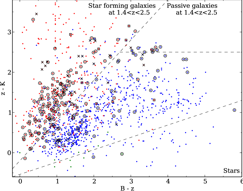
Figure 6: $B-z$ vs $z-K$ plot of all GMASS objects, showing which objects were included in the mask for spectroscopy. Colours indicate photometric redshift either above $z=1.4$ (red) or below $z=1.4$ (blue). Objects included for spectroscopy are marked by crosses (no redshift obtained), boxes (tentative redshift obtained), and circles (secure redshift obtained). Note that this includes mask fillers (at low redshift) and stars (for monitoring of the seeing and telescope pointing). The limits of the $BzK$ selection are indicated by dashed lines.

3.3 Observations

The observation blocks (OBs), including either two 30 minute (blue) or four 15 minute (red) exposures, were carried out in service mode under the following conditions: airmass $<$ 1.3 (blue) or 1.6 (red), lunar illumination $<$ 0.1 (blue) or 0.4 (red), distance to moon $>$ 60^∘ (blue) or 120^∘ (red), seeing $<$ 1$\aas@@fstack{\prime\prime}$0, and clear sky. Most of the OBs were carried out under photometric conditions. For each mask, at least one standard star was observed, under photometric conditions, before or after the science observations, using a long slit but otherwise the same set-up as the science observations. The overheads amounted to about 25% of the observing time, mainly because of the time spent during the acquisition procedure and on observations of the standard stars. In Table 2, we provide a precise account of the exposure times for each mask.

4 Reduction

The reduction of the 115 hour exposure of the six masks (and a few minutes of standard stars) was carried out using IRAF and IDL. We note that the CCDs were read out using on-chip pixel binning, resulting in images of 1024$\times$2048 pixels. When we refer to pixels in this section, we mean the latter (binned) pixels. The dispersion in the raw frames is therefore $\sim 3.4$ Å per pixel and the spatial scale 2$\aas@@fstack{\prime\prime}$5 per pixel in this section.

Since the blue and red masks were affected by different sky backgrounds and had different dithering patterns, the reduction differed in some ways between them, but the first few steps were equivalent.

First, an assessment of the data quality of each observed OB was done, including those that had been rejected by ESO. We used some of these rejected OBs. These were OBs taken under conditions slightly worse than requested (e.g., bad seeing). Adding these improved the quality of the co-added data, especially because we found several accepted OBs that were also taken under slightly worse conditions than requested.

As FORS2 is equipped with two CCDs, all of the reduction steps described below for the full frames were carried out for both CCDs. The spectral dispersion direction is along the horizontal direction on the CCDs.

4.1 Flat fields

We first treated the dome flat fields. These were taken for each night that science observations had been carried out. Between 5 and 20 flat-field frames were produced for each night. As the flat fields were very stable, we combined them all, making one flat field per mask. Bias values were subtracted by using the overscan region. Using IRAF’s response task, a 75th order cubic spline was fit interactively to the average of the lines of each separate slit. Each slit in the flat was then divided by its fit to form the normalized response function.

4.2 Wavelength calibration

Secondly, we treated the wavelength calibration frames. These were taken at the same time as the flats and enabled us to also check the instrumental stability. As they turned out to be stable too, we used the wavelength calibration frame for one night only for each mask. After bias subtraction, trimming, flat fielding, and the construction of a list of 24 (blue) and 20 (red) unblended lines out of the HeHgAr and HeAr line lists provided by IRAF, the observed lamp lines were identified interactively using IRAF’s identify and reidentify tasks. Starting from the bottom of the CCD, three lines were averaged, emission lines were identified, and a tenth-order Legendre polynomial was fit to obtain a dispersion solution. This procedure was repeated for each set of three lines, re-using the last dispersion solution obtained as long as the same slit was concerned, until the top of the CCD was reached. Depending on the position of the slit and therefore the actual wavelength coverage, typically fewer lines than the number of entries in the line list could be identified. The order of the polynomial fit was decreased for slits with fewer than 17 identified lines to ensure a plausible solution. An IDL procedure was written to divide the resulting database into separate parts for each slit, removing the first and last records, i.e. dismissing the first and last three lines of a slit as these were typically contaminated by emission lines from the neighbouring slit.

4.3 From masks to slits

Thirdly, we treated the science frames. These were bias subtracted and trimmed. Shifts in the dispersion direction between the frames were determined using three sky lines in three different slits (i.e. nine lines per frame). The shifts were of the order of one pixel. As the wavelength calibration is more accurate than one pixel, these shifts had to be corrected. The shifts in the spatial direction were determined using the bright object observed in the slit for dithering tracing. Apart from the dithering, shifts of up to several pixels were measured. These also had to be taken into account before the frames could be combined. As any non-integer pixel shifts involve interpolation that degrades the quality of the data, we preferred to carry out only one such step in the entire reduction process. This means that the distortion correction and the positional corrections had to be done at the same time. Interpolation of data containing cosmic rays leads to spreading of the cosmic rays over several pixels, which is much more difficult to remove than the cosmic rays in the original data. We experimented with several methods of cosmic ray detection and removal and found the method designed by van Dokkum (2001), based on a variation of Laplacian edge detection, to work best. This method works by first removing the sky lines using a low-order polynomial fit to the CCD columns and then identifies cosmic rays by subsampling the image and convolving with the appropriate kernel. This only works for single spectra, so we extracted the individual two-dimensional slit spectra from each frame before applying the procedure. We note that a mask with an average of 40 slits, observed for 30 hours at four dither positions, is represented by 4800 single files (called slits from now on) at this stage. The resulting cosmic-ray mask is kept for later use. The slits were subsequently flat fielded.

The rectification transformation was determined with IRAF’s fitcoords from the fits to the arc lamp lines made earlier using a two-dimensional Legendre polynomial of sixth order in the dispersion direction and second order in the spatial direction (note that an individual slit has typically only about 30 lines). In some cases, a fifth or seventh order was used in the dispersion direction, depending on the number of emission lines fit. Using the resulting rectification transformation solutions, the slits were interpolated to a linear wavelength scale with a dispersion of 2.5 Å per pixel, while at the same time the shifts in the spatial and dispersion directions were corrected so that the resulting rectified slits could be co-added without further corrections. Using eight unblended sky lines, the dispersion in the rectified slits was checked and found to be correct to within 0.5 pixels.

4.4 Co-addition and extraction of one-dimensional spectra

Before combining the individual frames, we computed the average airmass of all the frames together. First the airmasses at the beginning, middle, and end of each exposure were computed using the date and time, hour angle, and declination values obtained from the FITS header. The average airmass (AM) for an exposure was then computed by taking (AM(start) + 4$\times$AM(middle) + AM(end)) / 6. Finally, the airmasses of all frames were averaged to obtain the average airmass for the combined frame.

At this point, the individual files can be combined to form one file representing an exposure of up to 32 hours. There are different methods for performing this. We used different methods for the blue and red masks, following the different dithering strategies used. We experimented with various methods to compare the results, trying three methods for the blue masks and eight for the red masks, after which we decided which method to use for the final reduction. In the following, we describe the methods used for the blue and red masks.

4.4.1 Blue masks

For the blue masks, we carried out the following steps for each slit. First, all frames were averaged per dither position, without rejection (as cosmic rays had already been removed). Flux calibration, extinction correction, and telluric absorption correction were then applied to the two-dimensional frames. To remove the sky lines, IRAF’s background task was used, fitting a second-order Legendre polynomial (with four iterations to exclude deviant pixels from the fit) to all lines in a column. From a visual assessment of the background-subtracted two-dimensional image, the position(s) of the spectrum or spectra was (were) determined and the background subtraction was repeated on the original image using this information to exclude the lines containing the spectrum from the column fits. In principle, the two two-dimensional frames could now be averaged to form the final two-dimensional spectrum, but in almost all cases there were defects that had to be corrected by hand at this stage. These included the residuals of cosmic rays, CCD defects, bright sky lines from neighbouring slits, and slit edges. The latter two are particularly common in slits at the outer edges of the field of view. The applied distortion correction corrects only along the lines, which means that the strong distortion in FORS2 causes straight slits to be projected onto the CCD as curved stripes. As we created individual slit images using a fixed number of CCD lines per slit, unexposed pixels from regions outside the slit became visible at either short or long wavelengths, for some of the slits. One way to resolve this problem is to reduce the vertical size of the region on the image allocated to slits, but this would have reduced the area from which the background signal can be measured significantly as the deformation can lead to a difference in the vertical position of up to 1″ between the blue and red edges of a slit. The latter two effects and the first two when occurring outside the location of the spectrum of interest, caused undesired offsets in the background estimates. These were corrected by replacing the affected part of the column(s) by an unaffected part of the column(s), typically three pixels, and redoing the background subtraction, or excluding the affected lines from the background fit (for certain columns). If a defect occurred inside the region where the actual spectrum was located, it could not be replaced by another part of the column. In that case, it was replaced by the same two-dimensional region at the other dither position, reducing the S/N in this region in the final image by a factor of $\sqrt{2}$. Finally, one-dimensional spectra were extracted from the two-dimensional ones using unweighted summing over a 6 pixel (= 1$\aas@@fstack{\prime\prime}$5) aperture, unless there was clear evidence of a spatially extended source, in which case the aperture was broadened.

4.4.2 Red masks

For the red masks, we used a method similar to the one applied in the NIR, starting with the frames where cosmic rays were removed and flat fielding was carried out. In the following, the four dither positions are called A, B, C, and D. First, three dither positions (BCD, CDA, DAB, and ABC) were median-combined without shifting to form a representation of the sky background. These median frames were subtracted from the position that was not part of the median (A, B, C, and D, respectively). This should have taken care of the sky background removal, but owing to temporal variations in the strength of the sky lines some residuals remain. The frames were subsequently transformed to correct for the distortion. To remove the sky line residuals as well as possible, we used IRAF’s background task to fit a first-order Legendre polynomial (i.e. a line) to the columns and subtract this fit. As for the blue masks, this step was repeated once after the location of spectra in the two-dimensional frame had been determined, avoiding the lines containing the spectra. Finally, the sky-subtracted frames were averaged using a sigma-clipping rejection method and applying the appropriate shifts to obtain the final two-dimensional spectra. The two-dimensional spectra were flux-calibrated and corrected for extinction and telluric absorption. One-dimensional spectra were extracted from the two-dimensional ones using unweighted summing over a seven-pixel (= 1$\aas@@fstack{\prime\prime}$75) aperture, unless there was clear evidence of a spatially extended source, in which case the aperture was broadened.

4.5 Spectrophotometric calibration

Standard stars (LTT1788 and LTT3218) were observed during some (photometric) nights through 5″ slits. The observations of the standard stars were bias subtracted using the overscan regions and flat fielded using the flat fields taken for the 5″ slit. Distortion correction was also carried out using the dispersion solution obtained from the wavelength calibration frames for the 5″ slit. The observations of one standard star repeated over several nights were combined and a 14 pixel (or 3$\aas@@fstack{\prime\prime}$5) wide aperture was used to extract the spectrum, using a third- to fifth-order Legendre polynomial to trace the spectrum position. A response curve was determined using a standard star for each period (P73 or P74), by fitting a 15th order cubic spline to the parts of the standard-star observation unaffected by telluric absorption, while those parts affected were used to create a curve representing the telluric absorption. We attempted to create a telluric absorption curve from the brighter spectra in a science mask, but this turned out to be impossible as the S/N is insufficiently high.

Table 3: Average magnitude and flux difference between spectral and imaging photometry

Mask	Grism	$\Delta$mag		$\Delta$Flux
1	300I	0.23$\pm$	0.24	1.2$\pm$	0.3
2	300V	0.59$\pm$	0.20	1.7$\pm$	0.3
3	300V	0.58$\pm$	0.25	1.7$\pm$	0.4
4	300V	0.48$\pm$	0.25	1.6$\pm$	0.4
5	300I	0.13$\pm$	0.37	1.2$\pm$	0.4
6	300I	0.49$\pm$	0.28	1.6$\pm$	0.4

We computed synthetic spectral magnitudes by convolving the spectra with the HST/ACS $B_{435}$, $V_{606}$ and $i_{775}$ filters, wherever the spectra covered the full wavelength range of these filters. Five spectra cover only part of the $i_{775}$ filter and none of the others. Here we convolved only the appropriate part of the $i_{775}$ filter (which was more than 50% of its full width in all five cases). As expected, due to the more severe flux loss – caused by the finite width of the slits – for extended galaxies than for the unresolved standard stars, the synthetic magnitudes are in almost all cases higher than the imaging magnitudes, by 0.4 on average. The 3$\sigma$-clipped average offsets differ per mask and are listed in Table 3, together with the corresponding average ratio in flux. The obtained average values differ less than 0.1 mag from the median values (which were not $\sigma$-clipped). We excluded twelve outliers manually beforehand that were mostly serendipitous objects not centered in the slits and therefore suffer from additional slit losses. Also excluded were 14 objects for which imaging photometry is not available. The average offset is slightly higher for the bluer filters, by 0.1–0.2 mag. In Table LABEL:table:gmass_galaxies, we list the flux ratio per spectrum (averaged over multiple filters if available), that is also the multiplicative factor needed to normalise the spectra in order to obtain fluxes consistent with the imaging magnitudes.

4.6 Galaxies observed in multiple masks

To combine spectra of the targets that had been observed in multiple masks, we scaled the one-dimensional spectra using their common wavelength range, after which the common part of the spectra was averaged. Since the spectra had been flux-calibrated, we neither scaled nor weighted the spectra during the combination.

5 Spectroscopy results

5.1 One-dimensional spectra

One-dimensional spectra of galaxies for which we were able to determine a redshift (either secure or tentative, see below) are presented in Appendix B. All objects present in the GMASS catalogue that were observed spectroscopically are listed, together with their redshifts, photometry, and the Table in Appendix A.

5.2 Redshifts

5.2.1 Determination

Redshifts were principally determined by finding and identifying absorption and emission features in the galaxy spectra. In addition, once a sufficient number of redshifts had been determined for a mask, an average de-redshifted SED was constructed using the spectra with known redshifts and subsequently used to determine the redshift of galaxies for which the first method did not result in a redshift. Using the second method, only a few more redshifts were found and subsequently confirmed by identifying several spectral features that had not been noticed before. The quality of the redshifts determined was assessed, taking into account the number of features used and the S/N of these, resulting in three quality flags: (1) secure redshifts; (0) tentative redshifts, often based on only one spectral feature, very low S/N features, or discontinuities in the observed SED; and (-1) where no redshift could be determined.

Figure 7: Rest-frame composite spectra of galaxies in the blue (top) and red (bottom) masks. The most important absorption lines and one emission line ([O II]$\lambda$3727) are indicated. Note the clear difference in slope and strength of the FeII and MgII,MgI absorption lines.

In Fig. 7, we show composite spectra of blue (obtained in all masks) and red (obtained in the red masks only) galaxies, similar (but of higher S/N) to those used to determine the redshifts of individual galaxy spectra. During the co-addition to produce the composites, each spectrum was shifted to its rest-frame, rebinned to 1 Å bins, and normalized in the 3000-3500 Å (2000-2500 Å) wavelength range, which is always present in the observed spectroscopic window of the galaxies observed in the red (blue) masks.

5.2.2 Redshift determination success

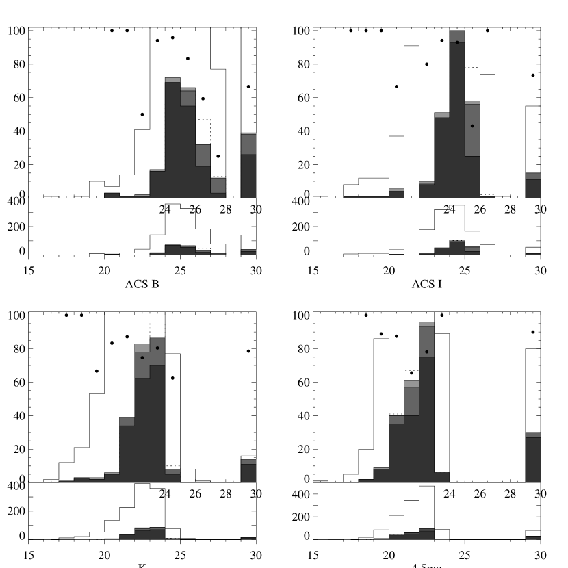
Figure 8: Magnitude histograms of the 1305 objects in the GMASS catalogue for the following bands: ACS $B$, ACS $I$, ISAAC $K_{s}$, and IRAC 4,5 $\mu$m (from left to right and top to bottom). The smaller histograms represent objects in the spectroscopic sample (dashed), those observed spectroscopically (light grey), those resulting in redshifts (grey), and those with secure redshifts (dark grey). The objects in the bin at magnitude 29.5 were not detected in the respective bands. Each panel contains the full histogram at the bottom, while the top histogram is a zoomed image of the spectroscopic sample and includes filled circles representing the secure spectroscopic redshift determination success rate per magnitude bin (in percentages). Note that the spectroscopic sample does not include objects with secure redshifts published in the literature.

In total, we were able to determine 135 secure redshifts (quality flag 1) for the 174 objects belonging to the spectroscopic target list and observed in at least one of the GMASS masks. In addition, 15 of these objects have less secure redshifts (quality flag 0). For 22 objects, the extracted spectra did not provide clues about their redshift or result in conflicting redshift determinations. Finally, two objects turned out to be too faint to allow extraction of their spectra. Among the objects with newly determined secure redshifts, 22 had been observed in previous surveys, but did not yet have secure redshifts. The success rate of redshift determination by GMASS is therefore 76% (86%, including less secure redshifts) for the full spectroscopic sample observed, 63% (76%) for the red sample, and 90% (94%) for the blue sample. We note that these rates would have been even higher, had we not excluded the (easier) targets in the GMASS field, for which redshifts had been previously determined in other surveys. The efficiency of selecting galaxies at $z>1.4$, i.e., the fraction for which $z_{\rm spec}>1.4$ among those with determined secure (tentative) redshifts is 89% (89%) for the complete sample, 84% (85%) for the red, and 94% (94%) for the blue sample. In Table 1, we list some more statistics, including the number of redshifts determined (at $z\geq 0$ and $z>1.4$) per sample.

Among the targets used to fill empty places in the masks, 40 objects were in the GMASS photometric catalogue, but had not been classified as spectroscopic targets. For 33 of these, we managed to obtain a secure redshift, 5 of these being at $z_{\rm spec}>1.4$. In addition, we extracted 41 spectra of sources not present in the GMASS photometric catalogue, most of these being serendipitously included in slits placed on other targets. We were able to determine 26 secure and 3 tentative redshifts for these fillers, 8 and 2 at $z_{\rm spec}>1.4$, respectively. These are also listed in Table 1.

In Fig. 8, we have plotted the number of redshifts determined as a function of magnitude, for several bands, in the form of histograms. The spectroscopic redshift determination success is relatively independent of the $K$ and 4.5 $\mu$m magnitudes, but is, as expected, a strong function of magnitude in the $B$ and $I$ bands, decreasing from $>$90% for $B,I<25$ to 25%, and 43% for $B>27$ and $I>25$, respectively.

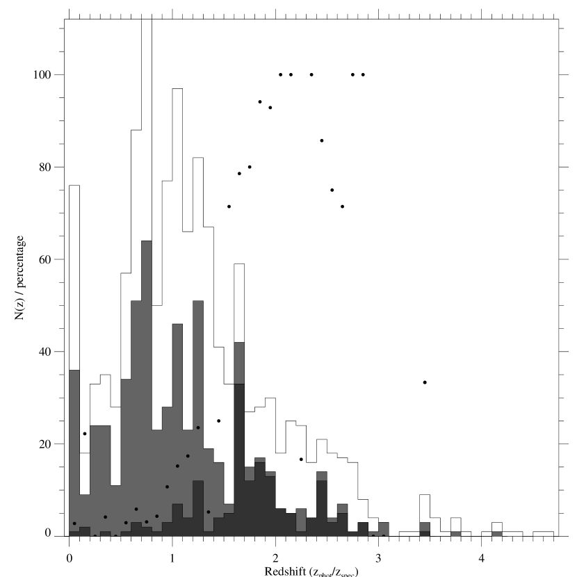
Figure 9: Histogram of redshifts in the GMASS catalogue. The open histogram represents photometric redshifts, while the grey (dark) histogram represents secure (GMASS only) spectroscopic redshifts. The dots indicate the percentage of secure redshifts determined by the GMASS survey.

In Fig. 9 (left panel), we have plotted a histogram of photometric and secure spectroscopic redshifts, both derived from GMASS observations and other surveys. We also indicate the ratio of spectroscopic redshifts derived from GMASS to the total number. It is clear that, within the GMASS field, at $z>1.5$ most redshift information comes only from GMASS, namely 120 out of the 152 (or 80%) spectroscopic redshifts, and, in the range $1.5<z<2.9$, 119 out of 145 (or 79%) redshifts. The redshift distribution is inhomogeneous: several peaks are visible in the histogram. The properties of the most significant high-redshift overdensity at $z=1.6$ are described in Kurk et al. (2009).

5.2.3 Comparison with photometric redshifts and BzK selection

In Fig. 4, we compare the newly obtained spectroscopic redshifts with both the early photometric redshifts (see Sec. 2.6) used for the sample selection and the more sophisticated photometric redshifts obtained later. We also show with dashed lines for both $z_{\rm phot}$ and $z_{\rm spec}$ equal to 1.4 the lower limit to our photometric redshift selection. The deviation of spectroscopic from the early (sophisticated) photometric redshifts for the new GMASS redshifts (bright [red] squares in the figure) is $\Delta(z)=0.021$ (-0.005) and $\sigma(\Delta(z))=0.041$ (0.021). This is a factor of two higher than the deviation from the training set of more than 300 spectroscopic redshifts in this field, most (92%) at $z\leq 1.4$. Indeed, the fraction of new $z_{\rm spec}>1.4$ that have $z_{\rm phot,early}(z_{\rm phot,soph.})>1.4$ is 94% (98%), while the fraction of new $z_{\rm spec}\leq 1.4$ that have $z_{\rm phot,early}(z_{\rm phot,soph.})\leq 1.4$ is 81% (92%).

As described in Sec. 2.6, the $BzK$ diagram can also be used to select galaxies at $1.4\la z\la 2.5$ with high efficiency and low contamination. The sample of known spectroscopic redshifts in the GMASS field (produced by GMASS and other surveys) confirms this: of the 570 objects with secure redshifts, 142 have $1.4<z_{\rm phot}\leq 2.5$ (110 of these, i.e. 77% have redshifts measured by GMASS) and 428 $z_{\rm phot}\leq 1.4$ or $z_{\rm phot}>2.5$. Of the former (latter) 124 (27) fall in the region allocated to $1.4\la z\la 2.5$ by the $BzK$ method (see also Fig. 5). The $BzK$ selection therefore seems to be efficient (82%) and to suffer only low contamination (18%). If the $BzK$ criteria are used to select $z>1.4$ galaxies, the contamination is only 11%. These percentages compare favourably to those computed for the larger sample of 1275 photometric redshifts, which were 69% and 31% (or 21% if we are not concerned about contamination by $z>2.5$ galaxies), respectively. The larger contamination among photometric redshifts may therefore be due to inaccuracies in the photometric redshift determination rather than due to $1.4\la z\la 2.5$ galaxies with colours inconsistent with the $BzK$ criteria. We note, however, that the galaxies with secure redshifts are a sub-sample of all galaxies within the $BzK$ region, which are probably biased towards brighter galaxies and/or with emission lines.

5.3 SED-derived properties of the GMASS samples

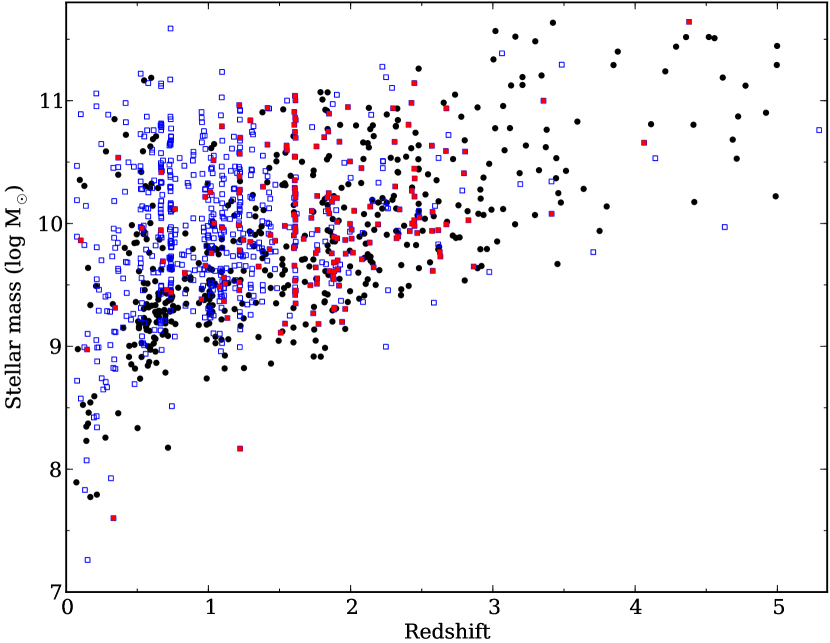
Figure 10: Stellar mass as a function of redshift in the GMASS catalogue. Galaxies with spectroscopic redshifts are identified by open [blue] squares. Those determined in the course of the GMASS survey are shown as filled [red] squares. Photometric redshifts are identified by the dark [black] filled circles.

Once the spectroscopic redshifts had been determined, new SED fits were obtained for the whole GMASS photometric catalogue, this time fixing the redshift parameter to the 609 spectroscopic redshifts (both secure and tentative) known, and leaving it as a free parameter for the other objects (resulting in a photometric redshift). During the fitting, observed magnitudes were used only up to rest-frame wavelength $\lambda_{0}$ = 2.5 $\mu$m to avoid the influence of dust emission (which was not included in the models used) and to minimise the effect that different stellar population synthesis models would have. No photometric shifts were applied in this fitting procedure, owing to uncertainties regarding their origin. We employed exponentially declining star formation histories, with characteristic times $\tau$ = 0.1, 0.3, 1, 2, 3, 5, 10, 15, and 30 Gyr, plus a model with a constant rate of star formation. A minimum age of 0.09 Gyr was imposed. We used only solar metallicities as we had found that introducing a choice of metallicities did not lead to a substantial improvement in the quality of the best-fits and produced differences in the best-fit stellar masses $\la 0.1$ dex, compared to solar metallicity SEDs, at the cost of introducing an additional parameter. We used values of extinction covering the range $0<A_{V}<4$. Moreover, we applied a prior in the choice of the best-fit models, similar to the one used by Fontana et al. (2004) and Bolzonella et al. (2010), that is, to exclude models with $A_{V}>0.6$ and age/$\tau>4$ (i.e., old galaxies must have a moderate dust extinction) and models with $\tau<0.6$ Gyr and ages for which $z_{\rm form}$ is $<1$ (to obtain a better estimate of the ages of early-type galaxies typically fitted by these low-$\tau$ models). In addition to the canonical stellar population models provided by Bruzual & Charlot (2003, BC03), we computed masses using the stellar population models of Maraston (2005), with the Kroupa initial mass function (IMF) (Kroupa 2001), similar to the Chabrier IMF (Chabrier 2003) used in Bruzual & Charlot models, and those by Charlot & Bruzual (Bruzual 2007a, b), both of which include the thermally pulsing asymptotic giant branch phase of stellar evolution. For intermediate age stellar populations, this phase can contribute up to $\sim$50% to the total bolometric light, radiated mostly in the NIR (e.g., Maraston 2005). The use of different SED models implies different mass estimates: for instance the change in the IMF from Chabrier to Salpeter produces higher estimates of the stellar masses (0.23 dex, i.e., a factor $\sim$1.7). In the remainder of this paper, when we refer to stellar masses, we refer to those computed using the BC03 models as these provide the best fits among the three models, and for consistency with previous works.

The stellar masses of observed galaxies and other galaxies in the GMASS photometric catalogue are shown in Fig. 10. The range of derived stellar masses for the galaxies with redshifts from GMASS observations is between 7.5 and 11.6 in log(M_⊙), with most (96%) galaxies being between 9.0 and 11.0 in log(M_⊙).

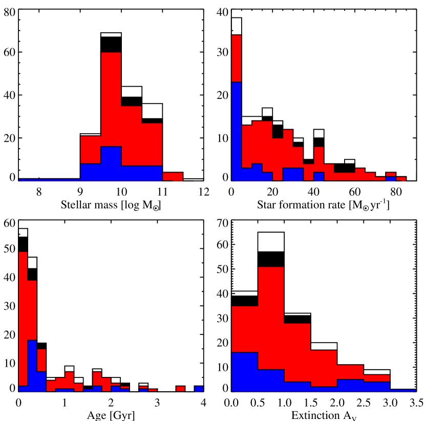
Figure 11: Histograms of SED-derived stellar masses, star formation rates, ages, and extinction (in A_V) for the sample with spectroscopic redshifts derived by GMASS (open histograms), secure spectroscopic redshifts derived by GMASS (filled histograms), for all redshifts (black), redshifts $z<2.0$ (red), and redshifts $z<1.4$ (blue). These histograms are plotted on top of each other, i.e., they are not cumulative.

In Fig. 11, we show histograms of SED-derived stellar masses, star formation rates, ages, and extinction (in A_V) for the sample with spectroscopic redshifts derived by GMASS (open histograms), secure spectroscopic redshifts derived by GMASS (filled histograms), for all redshifts (black), redshifts $z<2.0$ (red), and redshifts $z<1.4$ (blue). There are no obvious redshift differences in the distributions of mass and extinction. For star formation rates, the high-redshift galaxies have the highest star formation rates, while the lowest bin (SFR $<$ 5 M_⊙ yr^-1) is dominated by the galaxies at $z<1.4$. As the GMASS catalogue was selected on MIR magnitude, this difference in SFR can only be partly explained by selection effects. The highest redshift galaxies, have, as expected the lowest ages (most are younger than 0.4 Gyr).

5.4 Extending the CDFS spectroscopic catalogue

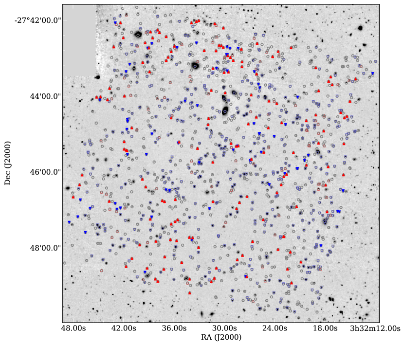
Figure 12: $K_{s}$-band image of the GMASS field in CDFS. Grey circles indicate the 1275 objects in the GMASS photometric catalogue. Blue downward pointing triangles indicate galaxies with spectroscopic redshifts $z<1.4$, while red upward pointing triangles indicate galaxies with spectroscopic redshifts $z\geq 1.4$. The triangles are filled if the redshift was determined by spectroscopy from the GMASS survey.

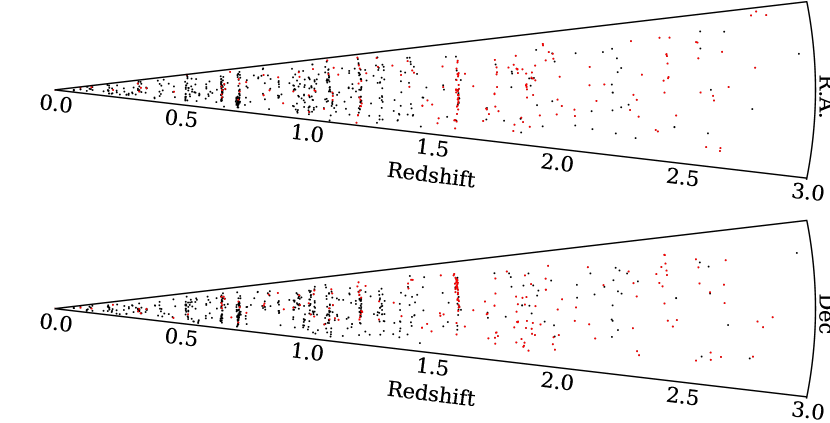
Figure 13: Cone plots showing the projection in R.A. in the top panel and declination in the bottom panel of the spatial distribution of galaxies in the GMASS field. Only galaxies with spectroscopic redshifts up to $z=3.0$ are shown. Red symbols indicate redshifts determined by spectroscopy from the GMASS survey. The angle of each cones was stretched by a factor of six to help visualisation.

As described in Sec. 2.7, the CDFS, in which the GMASS field is located, is the focus of many spectroscopic campaigns, providing thousands of galaxy redshifts. The GMASS survey provides additional spectra and redshifts, which fill an important niche in parameter space: its resulting redshifts are preferentially in the former redshift desert at $1.4<z<2.5$, and the galaxies are up to two magnitudes fainter ($B,I<26.0$) than those targeted in most other surveys, which explains the extremely long integration times needed ($\sim$ 30 hours). Balestra et al. (2010) compiled a master catalogue of spectroscopic redshifts obtained by 16 authors with 7332 entries. We extend this catalogue by 210 entries obtained by the GMASS project. Some of these (42) concern galaxies that had tentative redshifts from other surveys that are now replaced by more secure GMASS redshifts. In Fig. 12, we show the positions in the GMASS field of the galaxies with redshifts obtained by GMASS and other surveys. In Fig. 13, a redshift cone of galaxies in the GMASS field is displayed.

6 Notes on individual objects

Here we provide notes on individual objects, in particular those that have been detected at other wavelengths or observed by other surveys.

6.1 Radio sources

The CDFS was observed at 1.4 GHz using the Australian Telescope Compact Array down to a 1$\sigma$ limiting sensitivity of $\sim$14 $\mu$Jy (Koekemoer et al., in preparation). Within the area covered by the ACS observations, a total of 64 radio sources are found with 1.4 GHz fluxes between 63 $\mu$Jy and 20 mJy (Afonso et al. 2006). Afonso et al. (2006) identified these radio sources with objects detected on the ACS $z_{850}$ band using a likelihood method. Identifications were inspected visually to check for cases where the likelihood method might not apply. Seven of the radio sources were not identified with an optical source. We cross-correlated the GMASS catalogue with the catalogue published by Afonso et al. (2006), using the coordinates of the ACS counterpart, except for the seven cases without a counterpart, for which we used the coordinates of the radio source. All objects at distances smaller than 1$\aas@@fstack{\prime\prime}$0 were considered matches. Fourteen of these were found, all at distances $\leq$ 0$\aas@@fstack{\prime\prime}$3 and with optical identifications by Afonso et al.. Twelve of these already had secure spectroscopic redshifts determined by Szokoly et al. (2004), one has no spectroscopy at all, and one was observed in a GMASS mask. This last object – GMASS 2113, No. 24 in Afonso et al. – has a spectroscopic redshift of 1.613. Our spectrum of this galaxy displays a narrow [O II] emission line, but there is no evidence of broad lines. It has an extended, irregular morphology, with a colour gradient. As this galaxy is part of the redshift spike at $z=1.61$ in the GOODS-S field, its spectrum and HST image can be found in Kurk et al. (2009), where this spike is described in detail. This galaxy was also observed with SINFONI, the VLT’s NIR integral field spectrograph, displaying evidence of a merging system (Förster Schreiber et al. 2009), the clearest interacting system among the 63 galaxies detected in the SINS survey. We note that Kellermann et al. (2008) later also published deep radio observations of the CDFS, performed with the Very Large Array (VLA) at 20 and 6 cm, containing 266 sources. An even deeper VLA survey of Extended-CDFS is presented in Miller et al. (in prep.), containing 883 sources that are identified with optical/mid-IR sources and their spectroscopic and photometric redshifts by Bonzini et al. (submitted).

6.2 X-ray sources

Szokoly et al. (2004) carried out a spectroscopic survey of optical counterparts to X-ray sources in the CDFS, as observed by Chandra for 942 ks (Giacconi et al. 2002; Rosati et al. 2002). They used FORS2 with the 150I grism with typical exposure times of two to four hours. To check whether any of the new redshifts determined by the GMASS survey correspond to X-ray emitting sources, we cross-correlated the GMASS catalogue with the 1 Ms X-ray catalogue from Giacconi et al. (2002), using a distance of 1$\aas@@fstack{\prime\prime}$5 to match the coordinates, following Szokoly et al. (2004). The latter authors note that within this error circle, 0.15 field galaxies are expected to fall. That is, one false candidate is expected for every seventh X-ray source at $R<26$ (Vega magnitude).

There are four (possible) X-ray counterparts with either new or now confirmed formerly tentative redshifts:

GMASS 2443, 2043 These objects, at distances of 1$\aas@@fstack{\prime\prime}$40 and 1$\aas@@fstack{\prime\prime}$35 from their X-ray counterparts (Giacconi et al., Nos. 148, 231, resp.) were also observed by Szokoly et al. (2004, Nos. 241, 23, resp.) but they were unable to determine redshifts for these objects. We observed GMASS 2443 for a total of 44 h in two red masks and GMASS 2043 for 15 h in a blue mask, resulting in secure redshifts of $z=2.298$$\pm$0.004, and $z=2.576$$\pm$0.002, respectively. GMASS 2043 exhibits a broad emission line and has a compact morphology, suggesting that it is a QSO.

GMASS 1084 This object at 0$\aas@@fstack{\prime\prime}$96 distance from its X-ray counterpart (Giacconi et al., No. 227) was observed by Szokoly et al. (2004, No. 26, no redshift obtained) and Vanzella et al. (2006, No. 736, tentative redshift of $z=1.552$). We observed it for 15, 32, and 30 h in one blue and two red masks, respectively, resulting in a secure redshift of $z=1.552$$\pm$0.004.

GMASS 253 This object was also described by Daddi et al. (2005, No. 7, or 1446 in the UDF publicly available catalogue) as a high redshift elliptical with probable redshift of $z=2.47$. We observed this object for 30 h in a red mask, but were unable to secure its redshift, although our best estimate is $z=2.670$$\pm$0.001, close to that proposed by Daddi et al.. It is 1$\aas@@fstack{\prime\prime}$45 away from its X-ray counterpart (Giacconi et al., No. 224).

In addition, GMASS 1155 at $z=1.727$ has broad emission lines and a compact morphology, reminiscent of a QSO. It is listed as No. 145 without a redshift by Szokoly et al. (2004). Le Fèvre et al. (2004) report a redshift of $z=1.730$ for this source.

6.3 IEROS

Three IEROs (Yan et al. 2004) were included in the masks, but unfortunately their emission was too faint to determine unambiguous redshifts. One of these is GMASS 253, which was also described by Chen & Marzke (2004). It has a tentative GMASS redshift estimate of 2.670 (see Sec. 6.2), which is almost consistent with the photometric redshift of $>$2.8 determined by Chen & Marzke (2004) and is consistent with the redshift range $1.6<z<2.9$ given by Yan et al. (2004).

6.4 Objects from the K20 survey

As the GMASS field partly overlaps with that of the K20 survey (Cimatti et al. 2002a), eight objects previously selected for the K20 survey were included in the GMASS masks, one already having a secure redshift. For all K20 targets, secure redshifts could be determined from the GMASS observations, raising the number of K20 objects with secure redshifts from 501 to 508 and the spectroscopic redshift completeness of the K20 survey from 92% to 93% (508/545, Mignoli et al. 2005).

6.4.1 The deepest spectra

Five targets were observed in three different masks (none in four or more masks): GMASS 1084, 1314, 1380, 1788, and 2454. These objects were observed for 77, 62, 53, 55, and 77 h, respectively, resulting in secure redshifts of $z=1.552$$\pm$0.004, 2.007$\pm$0.002, 1.612$\pm$0.003, 3.413$\pm$0.003, and 1.602$\pm$0.002, respectively. Apart from GMASS 1084 described in Sec. 6.2, only GMASS 1380 had been observed before by Vanzella et al. (2006), who derived a tentative redshift of $z=1.611$ that we confirm ($z=1.612$$\pm$0.003). In addition, there are three targets observed in both masks r5 and r6, resulting in a total exposure time of 62 h: GMASS 1030, 1901, and 2239. None of these targets previously had spectroscopic data. Our observations resulted in a tentative redshift of $z=2.447$$\pm$0.003 for GMASS 1030, and secure redshifts of $z=0.1032$$\pm$0.0002, 1.415$\pm$0.002, respectively, for the others. We note that GMASS 1901 is a bright object with a point–like core that was used to position both masks and has data of the highest S/N among our spectra and quite likely the deepest spectrum ever taken for a $z\sim 0.1$ galaxy.

We are unaware of any other galaxy spectra, published in the literature, with exposure times of 60 hours or more and the data presented above are therefore likely the deepest galaxy spectra ever taken, with GMASS 1084 and GMASS 2454 being the record holders.

6.4.2 The faintest object with a secure redshift

The faintest object in the $K$ band with a secure redshift and m(4.5 $\mu$m)$<$23.0 is GMASS 2032 at $z=1.962$$\pm$0.005 and $K=24.1$, while the faintest object in the $I$ band is GMASS 1667 at $z=1.613$$\pm$0.002. The least luminous objects with secure redshifts are GMASS 365 and GMASS 408 for the $K$ and $I$ bands, at $z=1.609$$\pm$0.002, and 1.508$\pm$0.003 and $M_{K}=-21.0$ and $M_{I}=-20.7$, respectively.

6.4.3 The highest redshift objects

The most distant object for which a secure redshift could be derived from our observations is GMASS 1788 at $z=3.413$$\pm$0.003, described in Sec. 6.4.1, followed by GMASS 1160 at $z=2.865$$\pm$0.002, which forms the top of a more continuous redshift distribution down to $z=0$ (see also Fig. 9). We note that none of the forty targets with secure redshifts $z>2.00$ derived from GMASS observations had previously published secure (or even tentative) redshifts.

The highest redshift object with a tentative redshift is GMASS 2467 at $z=4.379$$\pm$0.006, observed for 32 h in a red mask. This redshift is based on the presence of two emission lines identified with Ly$\alpha$ and C IV, the latter being blue-shifted by 4500 km s^-1 w.r.t. to Ly$\alpha$. In the spectrum, there is a hint of continuum emission blueward of the tentative Ly$\alpha$ line, which would be uncommon for this redshift. In addition, in the $U$-band image, there seems to be emission from this galaxy, although a nearby much brighter object prevents a firm detection. If the bluest emission line were to be identified with C II, the redshift would be $z=2.384$, which is rather consistent with its photometric redshift of $z=2.3$. The second, redder, line should then be considered spurious, however, despite its S/N similar to that of the bluer line. We therefore prefer to list the two-line identification as tentative, but note $z=2.384$ as an alternative solution.

7 Public release

As originally stated in the proposal of this Large Programme, we make available for the general public the fully calibrated reduced spectra, both two- and one-dimensional, the corresponding two-dimensional fully calibrated sky background, and the GMASS catalogue. The GMASS catalogue contains both the photometric information on which the photometric redshifts are based as well as spectroscopic information, such as the redshift and its quality. The data can be accessed on a web page dedicated to GMASS. We have also updated the compilation of GOODS/CDFS spectroscopy master catalogue (now v3.0), available from the ESO website.

8 Summary

We have undertaken a spectroscopic survey of galaxies in CDFS, targeted specifically at galaxies selected in terms of mass at $z>1.4$. This field is one of most intensively imaged, from radio to X-ray wavelengths, and also the focus of extraordinary spectroscopic efforts. Nevertheless, the number of spectroscopic redshifts known in the range $1.5<z<2.5$ is relatively low, especially for galaxies that do not exhibit strong features related to on-going star formation. The spectra of these galaxies do not reveal sufficient detail in the typical exposures of a few hours to determine their redshift or other fundamental properties. We therefore carried out a spectroscopic survey, using one of the most sensitive optical multi-object spectrographs available at 8 m-class telescopes, FORS2 at the VLT, employing exceptionally long exposure times of 12 to 32 hours.

The galaxies targeted were all detected at m(4.5 $\mu$m)$<$23.0 to ensure that these were relatively massive (log($M/M_{\odot})\ga 10.5$ for $0<z<3$). The first release of the Spitzer/IRAC public imaging of the CDFS had just become available at the time we performed the target selection. The 4.5 $\mu$m photometry allows a more accurate estimate of the stellar mass than optical or NIR photometry and this channel also provides the best compromise amongst the four IRAC channels, in terms of sensitivity, PSF, image quality, and blending problems. Additional $U^{\prime},U,B,V,R,I,J,H$, and $K_{s}$ band photometry allowed us to determine accurate photometric redshifts. In addition to the 4.5 $\mu$m criterium, we selected the targets for spectroscopy based on (our own) photometric redshift $z_{\rm phot}>1.4$ and magnitude limits $B<26.5$ or $I<26.0$ for galaxies observed with the blue-sensitive 300V or red-sensitive 300I grisms, respectively. We excluded objects with known spectroscopic redshifts and those targeted by other spectroscopic surveys, but not yet observed at that time. These criteria left a sample of 221 targets, of which we could include 174 in three blue and three red spectroscopic masks. In addition, more than 46 objects were included to fill available spaces in the masks. We obtained exposure times from 11 to 32 hours per mask over the years from 2004 to 2006.

We reduced the spectra, ensuring that interpolation for wavelength calibration and rectification was performed only once. Background subtraction for the blue masks was performed in the way usually applied to optical spectra, while for the red masks we used a method similar to one applied in the NIR, taking advantage of having observed the spectra at four dither positions along the slits. Galaxy redshifts were determined by identifying absorption and emission features, and also by cross-correlating with composite galaxy spectra obtained from the sample of galaxies with known redshifts in the respective masks. Among the 244 objects for which we extracted one-dimensional spectra, we were able to determine 210 redshifts, of which 145 are at $z>1.4$, and 192 are securely identified. Among the 174 high-redshift galaxies targeted, we obtained redshifts for 150, of which 133 are at $z>1.4$, and 135 are securely identified. Within the field covered by GMASS, 80% of the known redshifts $z>1.5$ originate from our work, while the remainder is provided by the other numerous spectroscopic surveys within the CDFS. We extened the spectroscopic catalogue of the CDFS by 210 entries, 135 of which are new, 44 are more secure than determined in previous spectroscopy, and 31 are equal to existing entries. The redshift distribution has several noticeable peaks, the highest of which represents an overdensity of galaxies at $z=1.6$.

We have used the newly determined spectroscopic redshifts to assess the BzK selection criteria for selecting $z>1.4$ galaxies and found that these are efficient (82%) and suffer low contamination (11%). We used the GMASS spectra and extensive photometry in the CDFS to perform several studies, including that of quiescent superdense galaxies at $z>1.4$ (Cimatti et al. 2008; Cappellari et al. 2009), the stellar metallicity and outflows of star-forming $z\sim 2$ galaxies (Halliday et al. 2008, Talia et al., submitted), the evolution of the rest-frame colour distribution and dust properties of high redshift galaxies (Cassata et al. 2008; Noll et al. 2009), and the properties of galaxies in, and inflow of cold gas into, the galaxy overdensity at $z=1.6$ (Kurk et al. 2009; Giavalisco et al. 2011). The public release of the GMASS spectra will facilitate further studies of the distant galaxies targeted by our survey.

Appendix A Table of observed galaxies

Table 5: Galaxies observed in the GMASS masks: coordinates, photometry, redshifts, S/N, photometric normalisation factor, sample and mask(s)

ID	R.A.	Dec.	B		I		Ks		m4.5		$z_{\rm spec}$		q	S/N	Norm	S	M
2467	3:32:38.96	-27:42:43.7	99.00$\pm$	0.00	25.77$\pm$	0.30	21.57$\pm$	0.03	20.26$\pm$	0.01	4.3792$\pm$	0.0064	1	1.1	1.5	1	5
9111	3:32:16.07	-27:44:26.1	-		-		-		-		4.1365$\pm$	0.0061	0	0.3	0.0		5
418	3:32:33.03	-27:47:59.5	99.00$\pm$	0.00	25.04$\pm$	0.17	23.77$\pm$	0.13	22.66$\pm$	0.02	4.0627$\pm$	0.0062	0	0.9	2.2	1,3	6
1788	3:32:36.31	-27:44:34.6	25.94$\pm$	0.21	24.09$\pm$	0.07	23.08$\pm$	0.07	22.73$\pm$	0.02	3.4129$\pm$	0.0030	1	4.2	1.4	1,2	1,2,5
1807	3:32:19.05	-27:44:29.9	99.00$\pm$	0.00	25.94$\pm$	0.33	22.95$\pm$	0.06	21.03$\pm$	0.01	3.3561$\pm$	0.0012	0	0.6	2.0	1,3	5
9101	3:32:41.56	-27:45:26.5	-		-		-		-		3.1000$\pm$	0.0028	1	0.2	0.0		3
9102	3:32:41.91	-27:45:24.0	-		-		-		-		3.0711$\pm$	0.0067	1	0.1	0.0		3
1160	3:32:46.93	-27:46:04.7	25.40$\pm$	0.14	24.43$\pm$	0.10	23.86$\pm$	0.18	22.86$\pm$	0.02	2.8645$\pm$	0.0021	1	3.8	1.3	2,4	4
920	3:32:47.99	-27:46:39.5	24.51$\pm$	0.06	23.60$\pm$	0.05	22.90$\pm$	0.08	22.61$\pm$	0.02	2.8281$\pm$	0.0013	1	8.8	1.7	2,4	4
1048	3:32:47.23	-27:46:20.4	25.81$\pm$	0.20	24.67$\pm$	0.13	23.01$\pm$	0.11	22.09$\pm$	0.01	2.8054$\pm$	0.0027	1	1.6	2.7	1,2	2
307	3:32:35.05	-27:48:23.3	26.23$\pm$	0.26	25.34$\pm$	0.22	23.30$\pm$	0.08	22.35$\pm$	0.01	2.7973$\pm$	0.0040	1	1.6	2.3	1	2
9103	3:32:30.59	-27:42:39.5	-		-		-		-		2.6891$\pm$	0.0001	1	0.2	0.0		3
1980	3:32:14.99	-27:44:08.2	25.50$\pm$	0.13	24.75$\pm$	0.11	23.49$\pm$	0.11	22.79$\pm$	0.03	2.6734$\pm$	0.0017	1	5.1	1.1	2,4	4,5
1479	3:32:15.70	-27:45:15.4	25.77$\pm$	0.18	24.70$\pm$	0.12	22.53$\pm$	0.05	21.31$\pm$	0.01	2.6732$\pm$	0.0068	1	3.0	2.2	1,2	2,3
253	3:32:39.18	-27:48:32.3	27.08$\pm$	0.51	25.87$\pm$	0.34	22.78$\pm$	0.06	22.02$\pm$	0.01	2.6697$\pm$	0.0006	0	0.8	1.7	1,3	6
191	3:32:27.28	-27:48:45.7	24.34$\pm$	0.05	23.58$\pm$	0.05	23.33$\pm$	0.11	22.76$\pm$	0.02	2.6305$\pm$	0.0033	1	8.1	1.6	1,2	2
330	3:32:28.42	-27:48:19.0	24.66$\pm$	0.07	24.08$\pm$	0.07	23.68$\pm$	0.12	22.96$\pm$	0.02	2.6274$\pm$	0.0035	1	6.2	1.6	2	2
1796	3:32:15.64	-27:44:34.5	24.34$\pm$	0.05	23.88$\pm$	0.05	23.36$\pm$	0.11	22.28$\pm$	0.02	2.6161$\pm$	0.0037	1	11.6	2.0	2,4	3
2161	3:32:29.24	-27:42:58.9	26.46$\pm$	0.24	25.24$\pm$	0.16	23.97$\pm$	0.24	22.86$\pm$	0.03	2.5769$\pm$	0.0024	1	4.6	1.9	4	3
2043	3:32:41.88	-27:43:59.9	25.81$\pm$	0.19	24.92$\pm$	0.14	23.19$\pm$	0.09	22.05$\pm$	0.01	2.5763$\pm$	0.0021	1	2.4	1.8	2,4	4
167	3:32:37.89	-27:48:53.0	24.51$\pm$	0.06	23.79$\pm$	0.05	23.20$\pm$	0.10	22.48$\pm$	0.01	2.5729$\pm$	0.0016	1	7.1	2.0	2,4	4
2512	3:32:42.01	-27:42:27.8	26.87$\pm$	0.46	25.55$\pm$	0.25	23.58$\pm$	0.17	22.09$\pm$	0.01	2.5713$\pm$	0.0030	0	1.6	1.2	3	6
1049	3:32:23.18	-27:46:20.3	24.74$\pm$	0.07	24.12$\pm$	0.07	23.10$\pm$	0.08	22.56$\pm$	0.02	2.4832$\pm$	0.0018	1	5.6	1.9		4
885	3:32:43.69	-27:46:46.4	25.01$\pm$	0.14	24.79$\pm$	0.19	23.35$\pm$	0.10	23.01$\pm$	0.02	2.4677$\pm$	0.0059	1	3.8	1.4	2	2
2562	3:32:33.30	-27:42:01.9	25.73$\pm$	0.17	24.71$\pm$	0.13	22.57$\pm$	0.07	21.41$\pm$	0.01	2.4495$\pm$	0.0020	1	3.9	1.8	1,2,4	3,6
2207	3:32:36.89	-27:43:03.8	25.22$\pm$	0.11	24.77$\pm$	0.13	23.60$\pm$	0.17	21.75$\pm$	0.01	2.4488$\pm$	0.0018	1	7.9	1.1	2,4	3
2303	3:32:38.88	-27:43:21.5	24.58$\pm$	0.07	24.02$\pm$	0.07	23.34$\pm$	0.14	22.80$\pm$	0.03	2.4487$\pm$	0.0017	1	11.0	1.6	2,4	3
2363	3:32:39.41	-27:42:35.7	25.99$\pm$	0.22	24.51$\pm$	0.10	22.97$\pm$	0.10	21.79$\pm$	0.01	2.4485$\pm$	0.0005	1	3.0	1.5	2,4	6
2578	3:32:33.01	-27:42:00.5	25.55$\pm$	0.15	24.70$\pm$	0.13	22.00$\pm$	0.05	20.88$\pm$	0.01	2.4481$\pm$	0.0049	1	2.0	1.2	1	1
1030	3:32:39.34	-27:46:23.7	27.50$\pm$	0.70	25.57$\pm$	0.27	23.72$\pm$	0.14	22.88$\pm$	0.02	2.4469$\pm$	0.0027	0	1.5	1.4	1,3	5,6
1489	3:32:29.17	-27:45:14.8	25.44$\pm$	0.14	24.58$\pm$	0.09	23.25$\pm$	0.08	22.68$\pm$	0.02	2.4334$\pm$	0.0029	1	2.7	1.6	2	2
2471	3:32:32.36	-27:42:48.0	24.55$\pm$	0.06	23.79$\pm$	0.06	22.91$\pm$	0.11	22.08$\pm$	0.01	2.4301$\pm$	0.0024	1	9.3	2.2	2,4	3,4
1989	3:32:43.89	-27:44:05.8	24.46$\pm$	0.06	23.74$\pm$	0.05	21.67$\pm$	0.02	20.83$\pm$	0.01	2.4286$\pm$	0.0005	0	4.8	1.2	1,2	1
2090	3:32:18.72	-27:43:51.7	24.84$\pm$	0.08	24.20$\pm$	0.08	22.86$\pm$	0.07	22.11$\pm$	0.01	2.4164$\pm$	0.0011	1	6.0	1.7	2,4	4
2252	3:32:19.05	-27:43:15.2	25.52$\pm$	0.15	24.82$\pm$	0.13	22.66$\pm$	0.07	21.47$\pm$	0.01	2.4065$\pm$	0.0028	1	2.1	2.4	1,2	2
181	3:32:34.11	-27:48:49.6	24.10$\pm$	0.04	23.81$\pm$	0.06	23.07$\pm$	0.09	22.41$\pm$	0.01	2.3436$\pm$	0.0022	1	10.9	1.4	2,4	4
249	3:32:22.42	-27:48:33.6	25.97$\pm$	0.23	25.17$\pm$	0.16	23.47$\pm$	0.13	22.23$\pm$	0.01	2.3342$\pm$	0.0039	0	2.2	2.0	1,2,4	3
1711	3:32:27.11	-27:44:44.1	25.72$\pm$	0.18	25.09$\pm$	0.16	23.32$\pm$	0.08	22.69$\pm$	0.02	2.3235$\pm$	0.0040	1	4.7	1.8	2,4	3
2450	3:32:43.64	-27:43:47.9	24.99$\pm$	0.09	24.24$\pm$	0.09	22.70$\pm$	0.06	22.04$\pm$	0.01	2.3134$\pm$	0.0017	1	7.9	1.5	2,4	3
796	3:32:28.50	-27:46:58.2	26.16$\pm$	0.36	25.61$\pm$	0.32	22.49$\pm$	0.04	20.72$\pm$	0.01	2.3091$\pm$	0.0019	1	0.9	2.4	1,4	4
2443	3:32:24.20	-27:42:57.5	25.00$\pm$	0.10	24.42$\pm$	0.09	21.99$\pm$	0.04	21.10$\pm$	0.01	2.2979$\pm$	0.0037	1	5.0	1.0	1,2	1,5
2099	3:32:31.53	-27:43:50.9	24.95$\pm$	0.08	24.38$\pm$	0.08	23.06$\pm$	0.08	22.79$\pm$	0.03	2.1934$\pm$	0.0026	1	4.0	1.5	2	2
459	3:32:26.59	-27:47:50.1	25.39$\pm$	0.13	24.82$\pm$	0.12	23.39$\pm$	0.09	22.56$\pm$	0.02	2.1621$\pm$	0.0054	1	4.8	1.5	1,2	2,4
2572	3:32:36.89	-27:42:25.9	25.03$\pm$	0.10	24.29$\pm$	0.09	22.83$\pm$	0.09	22.02$\pm$	0.01	2.1375$\pm$	0.0028	1	7.2	1.6	1,2,4	3
881	3:32:31.32	-27:46:46.9	25.63$\pm$	0.16	25.22$\pm$	0.19	23.50$\pm$	0.10	23.09$\pm$	0.03	2.1336$\pm$	0.0018	1	3.8	1.3	2,4	4,6
1372	3:32:21.72	-27:45:29.6	25.59$\pm$	0.15	24.79$\pm$	0.14	23.24$\pm$	0.08	22.85$\pm$	0.03	2.0799$\pm$	0.0051	1	5.5	1.2	1,2,4	3
949	3:32:23.69	-27:46:32.9	25.54$\pm$	0.15	26.21$\pm$	0.42	23.42$\pm$	0.09	21.96$\pm$	0.01	2.0764$\pm$	0.0052	1	3.5	1.1	2,4	3,5
1663	3:32:24.73	-27:44:50.3	24.83$\pm$	0.11	24.23$\pm$	0.08	23.16$\pm$	0.08	22.43$\pm$	0.02	2.0249$\pm$	0.0032	1	6.5	1.9	2,4	3,6
502	3:32:34.14	-27:47:43.5	25.20$\pm$	0.11	24.70$\pm$	0.13	23.47$\pm$	0.11	22.70$\pm$	0.02	2.0156$\pm$	0.0032	1	2.6	2.1	2	2
149	3:32:21.95	-27:48:55.6	24.53$\pm$	0.06	23.85$\pm$	0.06	22.64$\pm$	0.05	21.93$\pm$	0.01	2.0069$\pm$	0.0018	1	8.4	1.9	2,4	3
1314	3:32:26.73	-27:45:40.0	24.97$\pm$	0.09	24.40$\pm$	0.08	23.39$\pm$	0.10	22.67$\pm$	0.02	2.0065$\pm$	0.0023	1	7.3	1.8	2,4	3,4,5
426	3:32:40.06	-27:47:55.4	24.46$\pm$	0.06	23.64$\pm$	0.05	21.65$\pm$	0.02	20.40$\pm$	0.01	1.9962$\pm$	0.0014	1	6.1	1.7	1,2	2
271	3:32:41.69	-27:48:29.6	24.73$\pm$	0.07	24.29$\pm$	0.09	23.07$\pm$	0.08	22.52$\pm$	0.01	1.9957$\pm$	0.0021	1	4.1	1.8	2	2
2559	3:32:42.34	-27:42:04.2	99.00$\pm$	0.00	25.39$\pm$	0.27	22.00$\pm$	0.04	20.71$\pm$	0.01	1.9807$\pm$	0.0014	0	1.1	1.9	1,3	1,6
2219	3:32:39.69	-27:43:06.6	23.66$\pm$	0.03	23.42$\pm$	0.04	22.90$\pm$	0.09	21.92$\pm$	0.01	1.9646$\pm$	0.0013	1	16.6	1.7	2,4	3
2032	3:32:45.19	-27:44:01.7	25.03$\pm$	0.09	24.46$\pm$	0.10	24.05$\pm$	0.18	22.67$\pm$	0.03	1.9622$\pm$	0.0046	1	2.8	1.9	2,4	2
2018	3:32:44.72	-27:44:01.4	24.36$\pm$	0.05	23.93$\pm$	0.06	22.89$\pm$	0.07	21.89$\pm$	0.01	1.9621$\pm$	0.0053	1	5.6	1.7	2	2
8005	3:32:21.35	-27:46:54.8	23.90$\pm$	0.03	23.71$\pm$	0.05	23.90$\pm$	0.27	22.89$\pm$	0.03	1.9403$\pm$	0.0030	1	15.5	1.5	2,4	3
472	3:32:38.12	-27:47:49.6	99.00$\pm$	0.00	25.99$\pm$	0.37	21.80$\pm$	0.02	21.04$\pm$	0.01	1.9213$\pm$	0.0037	1	1.2	1.1	1,3	6
1427	3:32:33.15	-27:45:22.8	25.91$\pm$	0.15	25.61$\pm$	0.21	23.63$\pm$	0.12	23.02$\pm$	0.03	1.9182$\pm$	0.0014	1	1.7	1.0	1,2	1,6
870	3:32:28.16	-27:46:48.4	25.32$\pm$	0.10	24.65$\pm$	0.10	23.20$\pm$	0.08	22.34$\pm$	0.01	1.9092$\pm$	0.0018	1	4.7	1.7	2,4	3
508	3:32:33.74	-27:47:44.2	24.93$\pm$	0.09	24.32$\pm$	0.09	23.00$\pm$	0.07	22.08$\pm$	0.01	1.9090$\pm$	0.0024	1	4.6	1.9	2,4	4
656	3:32:35.84	-27:47:18.7	24.58$\pm$	0.07	23.73$\pm$	0.05	22.35$\pm$	0.04	21.77$\pm$	0.01	1.9057$\pm$	0.0006	1	10.4	1.5	2,4	3
2275	3:32:17.28	-27:43:29.7	25.45$\pm$	0.14	24.77$\pm$	0.13	23.17$\pm$	0.12	22.34$\pm$	0.02	1.9050$\pm$	0.0033	1	1.1	1.1	1,2	1
90	3:32:34.09	-27:49:11.4	24.75$\pm$	0.08	24.29$\pm$	0.10	22.91$\pm$	0.07	21.53$\pm$	0.01	1.9029$\pm$	0.0023	1	4.0	1.8	2,4	4
923	3:32:27.26	-27:46:38.9	24.74$\pm$	0.11	24.39$\pm$	0.09	23.54$\pm$	0.11	22.82$\pm$	0.02	1.8849$\pm$	0.0014	1	8.1	1.7	2,4	3
2107	3:32:30.09	-27:42:42.9	24.76$\pm$	0.07	24.26$\pm$	0.08	23.49$\pm$	0.16	22.16$\pm$	0.02	1.8843$\pm$	0.0021	1	3.8	1.5	2,4	3,5
1789	3:32:31.84	-27:44:35.4	25.36$\pm$	0.10	24.53$\pm$	0.09	23.11$\pm$	0.08	22.11$\pm$	0.01	1.8834$\pm$	0.0014	1	3.3	1.8	2,4	4
250	3:32:30.91	-27:48:32.1	24.19$\pm$	0.06	23.96$\pm$	0.08	22.97$\pm$	0.07	22.33$\pm$	0.01	1.8828$\pm$	0.0016	1	5.8	1.7	2	2,6
679	3:32:35.52	-27:47:15.7	25.21$\pm$	0.12	24.63$\pm$	0.12	23.64$\pm$	0.12	23.01$\pm$	0.02	1.8827$\pm$	0.0019	1	4.4	1.5	2,4	4,6
183	3:32:31.16	-27:48:48.2	24.29$\pm$	0.07	23.74$\pm$	0.06	23.03$\pm$	0.08	22.42$\pm$	0.01	1.8820$\pm$	0.0013	1	9.2	1.6	2,4	4
118	3:32:31.53	-27:48:53.8	25.65$\pm$	0.18	24.79$\pm$	0.14	22.33$\pm$	0.04	20.87$\pm$	0.01	1.8795$\pm$	0.0041	1	1.8	2.4	1,2,4	4
1486	3:32:18.73	-27:45:14.4	23.80$\pm$	0.03	23.53$\pm$	0.04	22.86$\pm$	0.06	22.28$\pm$	0.02	1.8761$\pm$	0.0013	1	19.0	1.0	2,4	4,5
355	3:32:37.08	-27:48:14.4	26.94$\pm$	0.46	25.38$\pm$	0.23	23.42$\pm$	0.10	22.51$\pm$	0.01	1.8686$\pm$	0.0013	0	1.4	1.4	1,3	6
1748	3:32:20.20	-27:44:38.9	25.29$\pm$	0.12	24.79$\pm$	0.13	23.54$\pm$	0.11	22.55$\pm$	0.02	1.8668$\pm$	0.0023	1	2.8	2.0	2,4	4
894	3:32:35.82	-27:46:43.7	25.08$\pm$	0.08	24.48$\pm$	0.09	23.13$\pm$	0.07	22.25$\pm$	0.01	1.8502$\pm$	0.0020	1	4.6	1.8	2,4	3,6
220	3:32:37.18	-27:48:33.9	24.69$\pm$	0.07	23.79$\pm$	0.06	22.22$\pm$	0.04	21.08$\pm$	0.01	1.8499$\pm$	0.0013	1	4.7	1.7	2	2
875	3:32:37.09	-27:46:47.1	24.78$\pm$	0.08	24.40$\pm$	0.10	23.90$\pm$	0.15	-		1.8491$\pm$	0.0010	1	5.1	2.0		3
1498	3:32:41.91	-27:45:12.1	26.56$\pm$	0.35	25.63$\pm$	0.26	21.71$\pm$	0.02	20.72$\pm$	0.01	1.8478$\pm$	0.0016	0	1.4	0.9	1	1
858	3:32:37.36	-27:46:45.5	24.46$\pm$	0.06	23.76$\pm$	0.05	22.00$\pm$	0.03	21.11$\pm$	0.01	1.8463$\pm$	0.0017	1	8.4	1.7	1,2,4	3,4
1224	3:32:17.58	-27:45:51.8	26.78$\pm$	0.42	25.97$\pm$	0.35	21.95$\pm$	0.03	20.35$\pm$	0.01	1.8432$\pm$	0.0027	1	2.0	0.5	1,3	5
1822	3:32:15.35	-27:44:31.9	24.69$\pm$	0.07	24.32$\pm$	0.08	22.94$\pm$	0.07	22.45$\pm$	0.02	1.8419$\pm$	0.0022	1	5.7	1.9	2,4	4
675	3:32:38.81	-27:47:14.8	24.97$\pm$	0.09	24.16$\pm$	0.08	22.21$\pm$	0.03	21.16$\pm$	0.01	1.8361$\pm$	0.0076	1	3.3	1.9	1,2	2
2526	3:32:37.91	-27:42:15.4	26.60$\pm$	0.36	25.20$\pm$	0.19	22.11$\pm$	0.05	20.33$\pm$	0.01	1.8139$\pm$	0.0027	1	2.3	0.9	1,3	1,5
390	3:32:22.09	-27:48:06.7	24.02$\pm$	0.03	23.90$\pm$	0.05	23.55$\pm$	0.15	22.58$\pm$	0.02	1.7738$\pm$	0.0022	1	6.8	1.8	2	2
487	3:32:36.40	-27:47:47.0	23.85$\pm$	0.03	23.65$\pm$	0.06	22.53$\pm$	0.04	21.86$\pm$	0.01	1.7672$\pm$	0.0006	1	9.3	1.8	2,4	4
178	3:32:38.20	-27:48:49.4	25.25$\pm$	0.12	24.56$\pm$	0.11	22.97$\pm$	0.10	22.09$\pm$	0.01	1.7669$\pm$	0.0051	1	2.3	1.9	1,2	2
484	3:32:35.65	-27:47:48.8	23.83$\pm$	0.03	23.73$\pm$	0.05	23.23$\pm$	0.08	22.70$\pm$	0.02	1.7651$\pm$	0.0019	1	8.9	1.3	2	2
2403	3:32:30.95	-27:42:48.3	25.85$\pm$	0.20	24.56$\pm$	0.11	22.85$\pm$	0.09	21.96$\pm$	0.01	1.7647$\pm$	0.0020	1	1.8	1.4	1,2	1
335	3:32:40.99	-27:48:16.8	24.07$\pm$	0.04	23.89$\pm$	0.06	23.32$\pm$	0.09	22.67$\pm$	0.02	1.7626$\pm$	0.0016	1	6.9	1.7	2	2
1938	3:32:23.71	-27:44:11.8	24.70$\pm$	0.10	23.64$\pm$	0.05	21.59$\pm$	0.02	20.33$\pm$	0.01	1.7596$\pm$	0.0029	1	5.8	0.9	1,2	1
1464	3:32:28.31	-27:45:18.8	25.79$\pm$	0.18	24.85$\pm$	0.12	23.40$\pm$	0.10	21.95$\pm$	0.01	1.7552$\pm$	0.0039	1	2.7	2.6	1,2,4	3,4
1454	3:32:28.55	-27:45:19.4	27.38$\pm$	0.63	25.64$\pm$	0.22	23.47$\pm$	0.10	22.17$\pm$	0.01	1.7552$\pm$	0.0015	1	1.7	0.8	1,3	5
316	3:32:20.82	-27:48:22.5	23.78$\pm$	0.03	23.66$\pm$	0.05	23.33$\pm$	0.16	22.32$\pm$	0.01	1.7365$\pm$	0.0015	1	10.6	1.5	2	2
1155	3:32:22.54	-27:46:03.8	24.97$\pm$	0.09	24.22$\pm$	0.08	22.23$\pm$	0.04	20.40$\pm$	0.01	1.7269$\pm$	0.0029	1	3.8	1.5	1,2	1,5
1133	3:32:22.87	-27:46:07.2	25.05$\pm$	0.10	24.59$\pm$	0.11	23.03$\pm$	0.08	22.20$\pm$	0.02	1.7245$\pm$	0.0018	1	3.6	1.4	2	2
1624	3:32:18.11	-27:44:55.1	26.08$\pm$	0.23	25.17$\pm$	0.18	23.52$\pm$	0.11	22.32$\pm$	0.02	1.7166$\pm$	0.0036	0	1.2	1.3	1	1
1274	3:32:31.33	-27:45:44.7	25.47$\pm$	0.14	24.72$\pm$	0.12	22.64$\pm$	0.05	21.18$\pm$	0.01	1.6697$\pm$	0.0029	1	2.1	1.1	1,2	1
9112	3:32:36.31	-27:47:22.4	-		-		-		-		1.6390$\pm$	0.0008	0	0.4	0.0		6
1399	3:32:41.66	-27:45:25.6	25.54$\pm$	0.15	25.26$\pm$	0.19	23.79$\pm$	0.14	22.71$\pm$	0.02	1.6146$\pm$	0.0026	1	3.2	1.4	2,4	3
2196	3:32:36.67	-27:42:58.5	99.00$\pm$	0.00	25.13$\pm$	0.17	21.33$\pm$	0.02	20.34$\pm$	0.01	1.6138$\pm$	0.0038	1	1.2	2.0	3	6
1667	3:32:40.99	-27:44:50.2	26.25$\pm$	0.27	25.46$\pm$	0.23	23.76$\pm$	0.14	22.51$\pm$	0.02	1.6134$\pm$	0.0020	1	1.4	1.2	1	5
2540	3:32:30.33	-27:42:40.3	24.69$\pm$	0.07	24.02$\pm$	0.07	22.54$\pm$	0.07	21.40$\pm$	0.01	1.6128$\pm$	0.0015	1	4.1	1.1	2,4	3,6
2113	3:32:22.00	-27:42:43.5	26.18$\pm$	0.26	24.77$\pm$	0.13	22.15$\pm$	0.05	20.37$\pm$	0.01	1.6128$\pm$	0.0016	1	1.5	1.5	1	1
2368	3:32:17.10	-27:43:41.9	25.18$\pm$	0.11	24.44$\pm$	0.09	22.48$\pm$	0.07	21.15$\pm$	0.01	1.6121$\pm$	0.0014	1	3.5	1.9	1,2	2,4
1380	3:32:25.25	-27:45:29.0	24.91$\pm$	0.09	24.60$\pm$	0.09	22.99$\pm$	0.07	22.30$\pm$	0.02	1.6121$\pm$	0.0027	1	3.5	1.7	2	1,2,6
2603	3:32:27.85	-27:43:05.7	24.39$\pm$	0.06	23.80$\pm$	0.05	22.76$\pm$	0.08	21.74$\pm$	0.01	1.6120$\pm$	0.0008	1	12.1	1.6	2,4	3
2543	3:32:35.92	-27:42:41.0	99.00$\pm$	0.00	25.43$\pm$	0.18	21.53$\pm$	0.03	20.26$\pm$	0.01	1.6119$\pm$	0.0030	1	1.0	1.3	1,3	1
1691	3:32:31.90	-27:44:45.0	24.97$\pm$	0.08	24.12$\pm$	0.07	22.11$\pm$	0.03	21.11$\pm$	0.01	1.6119$\pm$	0.0009	1	4.0	1.9	1,2,4	4
1495	3:32:35.36	-27:45:12.6	25.17$\pm$	0.10	24.64$\pm$	0.10	22.50$\pm$	0.04	21.20$\pm$	0.01	1.6113$\pm$	0.0013	1	2.1	2.6	1,2,4	4
2055	3:32:26.77	-27:43:58.1	26.58$\pm$	0.36	25.49$\pm$	0.23	23.02$\pm$	0.07	22.21$\pm$	0.02	1.6112$\pm$	0.0015	1	1.8	1.0	1,3	6
1979	3:32:24.64	-27:44:07.8	24.12$\pm$	0.04	23.51$\pm$	0.04	22.10$\pm$	0.03	20.95$\pm$	0.01	1.6112$\pm$	0.0011	1	2.7	1.6	2	2
1254	3:32:20.17	-27:45:49.3	23.91$\pm$	0.03	23.71$\pm$	0.05	23.49$\pm$	0.10	22.21$\pm$	0.02	1.6105$\pm$	0.0013	1	7.1	1.7	2	2
2327	3:32:26.12	-27:43:25.0	25.39$\pm$	0.10	25.00$\pm$	0.13	23.88$\pm$	0.22	-		1.6103$\pm$	0.0014	1	1.6	1.9		6
2111	3:32:27.94	-27:42:45.7	99.00$\pm$	0.00	24.79$\pm$	0.13	21.52$\pm$	0.03	20.64$\pm$	0.01	1.6102$\pm$	0.0025	1	3.0	1.2	1	1,5
2142	3:32:23.54	-27:42:49.3	24.78$\pm$	0.08	24.34$\pm$	0.09	22.83$\pm$	0.09	22.22$\pm$	0.02	1.6098$\pm$	0.0028	1	7.1	1.0	2,4	4,5
2355	3:32:14.32	-27:43:32.9	26.48$\pm$	0.26	25.02$\pm$	0.14	21.91$\pm$	0.04	20.92$\pm$	0.01	1.6095$\pm$	0.0015	1	1.2	1.4	1	1
2251	3:32:29.48	-27:43:22.0	25.11$\pm$	0.10	24.28$\pm$	0.08	21.68$\pm$	0.03	20.64$\pm$	0.01	1.6094$\pm$	0.0019	1	6.2	1.6	1,2,4	3,6
2361	3:32:26.05	-27:42:36.6	99.00$\pm$	0.00	24.99$\pm$	0.15	21.25$\pm$	0.02	20.40$\pm$	0.01	1.6086$\pm$	0.0016	1	2.3	1.1	3	5
2247	3:32:27.86	-27:43:13.5	25.98$\pm$	0.19	24.81$\pm$	0.13	22.56$\pm$	0.07	21.77$\pm$	0.01	1.6086$\pm$	0.0007	0	1.9	1.1	1,2	1
2148	3:32:36.30	-27:42:49.5	27.15$\pm$	0.54	24.47$\pm$	0.10	20.90$\pm$	0.02	19.80$\pm$	0.01	1.6086$\pm$	0.0031	1	3.9	1.0	3	5
365	3:32:27.80	-27:48:12.0	24.43$\pm$	0.06	24.24$\pm$	0.08	23.72$\pm$	0.13	23.10$\pm$	0.02	1.6086$\pm$	0.0015	1	4.9	1.6		2
1808	3:32:26.15	-27:44:33.3	24.84$\pm$	0.09	24.28$\pm$	0.08	23.24$\pm$	0.09	22.61$\pm$	0.02	1.6085$\pm$	0.0012	1	4.8	1.6		4,6
2180	3:32:29.56	-27:42:56.0	24.59$\pm$	0.05	23.72$\pm$	0.04	22.00$\pm$	0.04	21.00$\pm$	0.01	1.6077$\pm$	0.0016	1	9.1	2.0	1,2,4	3,6
2493	3:32:38.51	-27:42:28.0	24.48$\pm$	0.04	23.67$\pm$	0.04	22.10$\pm$	0.05	20.88$\pm$	0.01	1.6073$\pm$	0.0016	1	8.4	1.8	2,4	3
1708	3:32:23.12	-27:44:42.2	99.00$\pm$	0.00	25.27$\pm$	0.19	22.22$\pm$	0.03	20.81$\pm$	0.01	1.6069$\pm$	0.0012	1	1.3	1.7	1,3	1,5
781	3:32:17.71	-27:47:02.9	23.77$\pm$	0.03	23.67$\pm$	0.05	23.40$\pm$	0.15	22.54$\pm$	0.02	1.6052$\pm$	0.0016	1	9.1	1.5	2	2
2352	3:32:33.88	-27:42:04.1	25.10$\pm$	0.10	24.15$\pm$	0.08	21.31$\pm$	0.02	20.09$\pm$	0.01	1.6042$\pm$	0.0027	1	3.6	1.0	1,2	1
2286	3:32:29.99	-27:43:22.6	99.00$\pm$	0.00	25.20$\pm$	0.17	21.80$\pm$	0.04	20.82$\pm$	0.01	1.6036$\pm$	0.0025	1	1.9	1.1	3	5
2454	3:32:28.91	-27:43:03.6	25.31$\pm$	0.11	24.41$\pm$	0.09	22.24$\pm$	0.05	20.80$\pm$	0.01	1.6019$\pm$	0.0015	1	4.0	1.2	1,2,4	4,5,6
2341	3:32:17.52	-27:43:36.6	24.55$\pm$	0.06	24.21$\pm$	0.08	23.35$\pm$	0.16	22.47$\pm$	0.02	1.6018$\pm$	0.0037	1	7.7	2.1	2,4	3
2550	3:32:30.08	-27:42:12.2	24.78$\pm$	0.07	24.14$\pm$	0.08	23.02$\pm$	0.11	22.03$\pm$	0.01	1.6012$\pm$	0.0015	1	7.7	1.6	2,4	3
2081	3:32:29.86	-27:43:54.8	24.37$\pm$	0.06	24.53$\pm$	0.10	23.57$\pm$	0.14	22.09$\pm$	0.01	1.6011$\pm$	0.0010	1	4.5	1.4	2	2
1084	3:32:39.74	-27:46:11.5	26.42$\pm$	0.31	25.16$\pm$	0.19	21.64$\pm$	0.02	19.73$\pm$	0.01	1.5518$\pm$	0.0037	1	1.5	1.8	1,4	4,5,6
2573	3:32:31.10	-27:42:05.3	26.55$\pm$	0.33	24.74$\pm$	0.13	21.97$\pm$	0.04	20.06$\pm$	0.01	1.5496$\pm$	0.0013	1	1.8	1.3	1	1
1050	3:32:17.88	-27:46:20.8	24.57$\pm$	0.06	24.10$\pm$	0.07	23.77$\pm$	0.20	22.61$\pm$	0.02	1.5392$\pm$	0.0022	1	5.9	2.5	2,4	3
1146	3:32:15.75	-27:46:04.6	24.92$\pm$	0.09	24.05$\pm$	0.07	22.08$\pm$	0.04	20.86$\pm$	0.01	1.5368$\pm$	0.0017	1	7.7	1.8	1,2,4	3
408	3:32:23.56	-27:48:02.6	24.94$\pm$	0.08	24.46$\pm$	0.10	23.79$\pm$	0.13	22.89$\pm$	0.02	1.5076$\pm$	0.0033	1	2.9	2.0	2	2
685	3:32:25.33	-27:47:15.5	25.74$\pm$	0.17	25.62$\pm$	0.27	24.61$\pm$	0.26	-		1.4877$\pm$	0.0007	1	1.0	1.0		1
512	3:32:22.84	-27:47:42.5	26.83$\pm$	0.42	25.55$\pm$	0.26	22.94$\pm$	0.07	21.97$\pm$	0.01	1.4692$\pm$	0.0001	1	1.9	0.8	1,3	5
9110	3:32:22.90	-27:47:42.3	-		-		-		-		1.4685$\pm$	0.0007	1	1.3	0.0		5
2484	3:32:37.69	-27:42:19.5	24.98$\pm$	0.09	24.09$\pm$	0.07	22.58$\pm$	0.07	21.59$\pm$	0.01	1.4356$\pm$	0.0008	1	4.3	1.7	2,4	4
2381	3:32:38.77	-27:42:18.4	25.50$\pm$	0.15	24.54$\pm$	0.11	22.83$\pm$	0.09	21.55$\pm$	0.01	1.4302$\pm$	0.0009	0	3.2	2.1	2,4	3
2470	3:32:43.15	-27:42:42.1	99.00$\pm$	0.00	24.15$\pm$	0.07	21.15$\pm$	0.02	20.16$\pm$	0.01	1.4156$\pm$	0.0019	1	4.7	1.1	1,3	5
2239	3:32:31.32	-27:43:16.2	99.00$\pm$	0.00	24.93$\pm$	0.15	21.58$\pm$	0.03	20.61$\pm$	0.01	1.4151$\pm$	0.0018	1	2.6	1.5	3	5,6
996	3:32:36.92	-27:46:28.5	99.00$\pm$	0.00	25.56$\pm$	0.26	22.14$\pm$	0.03	21.36$\pm$	0.01	1.3844$\pm$	0.0032	0	1.6	1.3	3	5
1652	3:32:41.58	-27:44:52.8	24.98$\pm$	0.10	24.93$\pm$	0.15	23.44$\pm$	0.11	23.01$\pm$	0.03	1.3527$\pm$	0.0015	1	4.0	1.2	2,4	4
793	3:32:45.98	-27:46:57.7	24.61$\pm$	0.07	23.86$\pm$	0.06	22.31$\pm$	0.05	21.73$\pm$	0.01	1.2951$\pm$	0.0014	1	4.6	1.7		2
1682	3:32:41.50	-27:44:40.2	26.92$\pm$	0.45	24.63$\pm$	0.11	21.12$\pm$	0.01	19.84$\pm$	0.01	1.2950$\pm$	0.0010	1	3.1	1.1	3	6
2135	3:32:38.60	-27:42:37.0	25.31$\pm$	0.12	24.55$\pm$	0.11	22.64$\pm$	0.07	21.70$\pm$	0.01	1.2458$\pm$	0.0002	1	3.2	1.4	2,4	4
9107	3:32:22.74	-27:46:02.6	-		-		-		-		1.2273$\pm$	0.0008	1	1.0	0.0		1
1217	3:32:21.23	-27:45:54.8	24.28$\pm$	0.05	24.03$\pm$	0.07	23.45$\pm$	0.10	-		1.2251$\pm$	0.0016	1	4.7	1.8		2
1952	3:32:34.65	-27:44:08.1	25.94$\pm$	0.21	24.19$\pm$	0.07	20.98$\pm$	0.01	20.04$\pm$	0.01	1.2239$\pm$	0.0063	1	4.5	1.2	3	5
1227	3:32:21.30	-27:45:54.6	24.57$\pm$	0.06	24.24$\pm$	0.08	23.76$\pm$	0.13	22.65$\pm$	0.02	1.2232$\pm$	0.0014	1	4.3	1.8	2	2
2235	3:32:41.25	-27:43:09.7	99.00$\pm$	0.00	25.54$\pm$	0.26	22.11$\pm$	0.05	20.80$\pm$	0.01	1.2216$\pm$	0.0014	1	1.4	1.3	3	5
1020	3:32:24.60	-27:46:20.3	26.66$\pm$	0.37	23.92$\pm$	0.06	21.16$\pm$	0.01	20.17$\pm$	0.01	1.2209$\pm$	0.0017	1	4.5	1.3		4
2580	3:32:42.97	-27:42:04.2	24.89$\pm$	0.06	23.89$\pm$	0.06	22.74$\pm$	0.08	21.58$\pm$	0.01	1.2199$\pm$	0.0008	1	4.2	1.1		1
886	3:32:47.14	-27:46:44.4	27.30$\pm$	0.64	25.06$\pm$	0.18	21.68$\pm$	0.03	20.92$\pm$	0.01	1.2193$\pm$	0.0003	1	2.0	1.6	3	6
774	3:32:16.45	-27:47:02.3	23.92$\pm$	0.04	23.44$\pm$	0.04	22.64$\pm$	0.08	22.35$\pm$	0.02	1.2171$\pm$	0.0015	1	6.5	2.1		2
773	3:32:16.26	-27:47:03.2	24.33$\pm$	0.05	24.04$\pm$	0.07	23.32$\pm$	0.14	22.66$\pm$	0.02	1.2169$\pm$	0.0022	1	3.1	2.8		2
2092	3:32:25.74	-27:43:47.1	99.00$\pm$	0.00	24.24$\pm$	0.08	20.93$\pm$	0.01	19.89$\pm$	0.01	1.2168$\pm$	0.0015	1	3.9	1.7	3	6
2283	3:32:12.27	-27:43:24.3	99.00$\pm$	0.00	25.72$\pm$	0.28	22.10$\pm$	0.04	20.99$\pm$	0.01	1.2161$\pm$	0.0007	0	0.5	1.7	1	1
2231	3:32:33.28	-27:42:36.1	99.00$\pm$	0.00	25.46$\pm$	0.22	22.66$\pm$	0.08	21.73$\pm$	0.01	1.2131$\pm$	0.0003	1	0.9	2.2	1,3	6
712	3:32:38.64	-27:47:11.5	24.80$\pm$	0.08	24.04$\pm$	0.07	23.18$\pm$	0.08	22.55$\pm$	0.02	1.1338$\pm$	0.0015	1	4.6	1.5		6
795	3:32:42.77	-27:46:59.1	24.03$\pm$	0.05	23.52$\pm$	0.05	22.65$\pm$	0.05	22.51$\pm$	0.01	1.1191$\pm$	0.0016	1	6.9	1.8		2
1567	3:32:24.01	-27:45:04.0	24.71$\pm$	0.07	23.97$\pm$	0.06	22.90$\pm$	0.06	22.74$\pm$	0.02	1.1101$\pm$	0.0023	1	5.2	1.4		2
2158	3:32:26.38	-27:43:21.5	24.30$\pm$	0.05	23.64$\pm$	0.05	22.93$\pm$	0.10	22.62$\pm$	0.02	1.1097$\pm$	0.0006	1	5.1	1.1		1
9108	3:32:28.31	-27:42:44.4	-		-		-		-		1.1080$\pm$	0.0002	1	0.9	0.0		1
692	3:32:47.44	-27:47:11.1	26.77$\pm$	0.42	24.64$\pm$	0.12	21.86$\pm$	0.03	21.00$\pm$	0.01	1.0981$\pm$	0.0019	1	2.6	1.2	3	5
1315	3:32:39.26	-27:45:32.3	25.58$\pm$	0.16	23.44$\pm$	0.04	20.65$\pm$	0.01	19.74$\pm$	0.01	1.0952$\pm$	0.0007	1	5.5	1.4		4
428	3:32:18.44	-27:47:57.0	24.05$\pm$	0.04	23.36$\pm$	0.04	22.38$\pm$	0.06	22.02$\pm$	0.01	1.0793$\pm$	0.0011	1	7.4	2.9		3
2191	3:32:29.29	-27:42:44.8	25.82$\pm$	0.16	23.94$\pm$	0.05	21.80$\pm$	0.04	21.23$\pm$	0.01	1.0404$\pm$	0.0015	1	5.6	0.9		1
9105	3:32:29.61	-27:43:20.3	-		-		-		-		1.0356$\pm$	0.0001	0	0.3	0.0		3
839	3:32:42.98	-27:46:50.0	99.00$\pm$	0.00	24.35$\pm$	0.09	21.10$\pm$	0.01	20.28$\pm$	0.01	1.0356$\pm$	0.0010	1	5.6	0.9	3	5
983	3:32:15.79	-27:46:29.9	23.31$\pm$	0.02	22.63$\pm$	0.02	21.94$\pm$	0.04	21.05$\pm$	0.01	1.0210$\pm$	0.0007	1	22.6	2.1	2,4	3
1704	3:32:26.43	-27:44:43.7	99.00$\pm$	0.00	24.87$\pm$	0.14	21.54$\pm$	0.02	20.61$\pm$	0.01	1.0143$\pm$	0.0021	1	1.6	2.0	3	6
1585	3:32:38.59	-27:45:00.0	24.71$\pm$	0.07	23.68$\pm$	0.05	22.40$\pm$	0.04	22.08$\pm$	0.01	0.9789$\pm$	0.0024	1	5.6	1.6		4
2296	3:32:41.68	-27:43:21.5	99.00$\pm$	0.00	24.89$\pm$	0.14	21.91$\pm$	0.04	20.94$\pm$	0.01	0.9783$\pm$	0.0015	1	1.9	1.0		1
1394	3:32:28.90	-27:45:25.4	23.71$\pm$	0.03	22.92$\pm$	0.02	22.54$\pm$	0.04	22.43$\pm$	0.02	0.9520$\pm$	0.0003	1	1.7	10.2		6
1309	3:32:20.39	-27:45:42.1	25.63$\pm$	0.16	24.49$\pm$	0.10	24.43$\pm$	0.23	-		0.9143$\pm$	0.0017	1	2.3	1.3		1
2461	3:32:39.09	-27:42:44.2	23.53$\pm$	0.03	22.77$\pm$	0.02	22.36$\pm$	0.06	-		0.8939$\pm$	0.0007	1	9.8	1.7		5
9113	3:32:29.60	-27:42:54.6	-		-		-		-		0.8570$\pm$	0.0007	1	0.6	0.0		6
9114	3:32:41.53	-27:44:36.8	-		-		-		-		0.8373$\pm$	0.0001	1	0.6	0.0		6
1579	3:32:25.76	-27:44:59.3	24.12$\pm$	0.05	23.03$\pm$	0.03	21.91$\pm$	0.03	-		0.8335$\pm$	0.0008	1	13.2	1.8		4
1592	3:32:25.80	-27:45:00.0	24.78$\pm$	0.08	23.81$\pm$	0.05	22.45$\pm$	0.04	21.43$\pm$	0.01	0.8319$\pm$	0.0004	1	8.6	1.8	2,4	4,6
942	3:32:36.49	-27:46:29.2	23.61$\pm$	0.03	22.26$\pm$	0.01	21.44$\pm$	0.02	21.04$\pm$	0.01	0.7649$\pm$	0.0003	1	24.0	1.4		5
1501	3:32:35.45	-27:45:14.3	26.42$\pm$	0.30	24.84$\pm$	0.12	23.91$\pm$	0.15	-		0.7380$\pm$	0.0006	1	1.2	2.1		4
9109	3:32:28.41	-27:45:19.2	-		-		-		-		0.7375$\pm$	0.0003	1	0.8	0.0		5
210	3:32:39.43	-27:48:38.8	25.53$\pm$	0.15	23.81$\pm$	0.06	22.31$\pm$	0.05	22.01$\pm$	0.01	0.7361$\pm$	0.0032	1	4.1	1.6		2
9106	3:32:21.23	-27:44:01.7	-		-		-		-		0.7344$\pm$	0.0002	1	0.8	0.0		1
558	3:32:46.54	-27:47:35.9	24.62$\pm$	0.07	23.19$\pm$	0.03	22.18$\pm$	0.04	22.63$\pm$	0.02	0.7064$\pm$	0.0012	1	6.2	1.9		2
2223	3:32:30.89	-27:43:16.1	25.16$\pm$	0.11	22.99$\pm$	0.03	21.71$\pm$	0.03	-		0.6799$\pm$	0.0001	1	1.7	10.0		5
2109	3:32:35.60	-27:42:43.3	25.74$\pm$	0.13	24.25$\pm$	0.07	23.85$\pm$	0.21	-		0.6766$\pm$	0.0003	1	2.4	1.4		1
1700	3:32:22.66	-27:44:45.2	24.90$\pm$	0.09	23.69$\pm$	0.05	23.27$\pm$	0.09	-		0.6677$\pm$	0.0007	1	1.1	5.6		1
2357	3:32:29.64	-27:42:42.6	22.48$\pm$	0.01	20.97$\pm$	0.00	19.82$\pm$	0.01	19.47$\pm$	0.01	0.6676$\pm$	0.0009	1	30.2	2.1		1
1388	3:32:25.57	-27:45:28.9	26.04$\pm$	0.32	24.47$\pm$	0.08	24.00$\pm$	0.17	-		0.6669$\pm$	0.0002	1	2.7	1.6		2
1920	3:32:33.17	-27:44:15.2	26.65$\pm$	0.36	23.54$\pm$	0.04	21.56$\pm$	0.02	21.71$\pm$	0.01	0.6657$\pm$	0.0007	1	4.5	1.9		4
643	3:32:48.47	-27:47:19.7	24.84$\pm$	0.08	22.53$\pm$	0.02	21.12$\pm$	0.02	21.45$\pm$	0.01	0.5328$\pm$	0.0007	1	13.3	1.8		4
192	3:32:27.42	-27:48:45.8	25.73$\pm$	0.17	24.63$\pm$	0.12	24.11$\pm$	0.21	-		0.4758$\pm$	0.0026	1	1.0	0.0		2
1232	3:32:32.97	-27:45:45.6	23.18$\pm$	0.02	20.41$\pm$	0.00	19.07$\pm$	0.00	-		0.3659$\pm$	0.0005	1	62.8	1.7		2
453	3:32:33.83	-27:47:48.0	23.66$\pm$	0.03	22.14$\pm$	0.01	21.38$\pm$	0.02	21.73$\pm$	0.01	0.3444$\pm$	0.0006	1	3.6	11.0		4
1304	3:32:26.89	-27:45:42.0	25.11$\pm$	0.10	23.85$\pm$	0.05	23.69$\pm$	0.12	-		0.3373$\pm$	0.0001	1	0.7	10.2		4
815	3:32:42.35	-27:46:57.2	26.02$\pm$	0.24	24.93$\pm$	0.16	23.53$\pm$	0.11	22.30$\pm$	0.01	0.3331$\pm$	0.0002	1	2.5	1.7	1,4	4
9104	3:32:29.70	-27:42:54.5	-		-		-		-		0.2325$\pm$	0.0001	1	1.5	0.0		3
1323	3:32:41.52	-27:45:32.5	21.80$\pm$	0.01	20.73$\pm$	0.00	20.46$\pm$	0.01	20.84$\pm$	0.01	0.1469$\pm$	0.0001	1	57.5	1.2		1
1901	3:32:44.80	-27:44:06.4	20.90$\pm$	0.00	19.14$\pm$	0.00	18.48$\pm$	0.00	18.94$\pm$	0.01	0.1032$\pm$	0.0002	1	1002.2	0.6		5,6
750	3:32:31.74	-27:46:58.4	20.55$\pm$	0.00	18.83$\pm$	0.00	18.67$\pm$	0.00	19.98$\pm$	0.01	0.0004$\pm$	0.0003	1	280.0	1.4		4
1277	3:32:19.95	-27:45:33.7	20.10$\pm$	0.00	17.93$\pm$	0.00	17.37$\pm$	0.00	18.53$\pm$	0.01	0.0002$\pm$	0.0005	1	603.1	1.7		3
2246	3:32:25.90	-27:43:41.2	25.13$\pm$	0.11	20.22$\pm$	0.00	18.27$\pm$	0.00	19.17$\pm$	0.01	0.0001$\pm$	0.0004	1	4.0	22.7		6
1581	3:32:25.76	-27:45:01.7	23.02$\pm$	0.02	22.20$\pm$	0.01	22.58$\pm$	0.05	-		0.0000$\pm$	0.0001	1	21.7	1.7		6
2494	3:32:21.04	-27:43:10.2	24.01$\pm$	0.04	20.79$\pm$	0.00	20.92$\pm$	0.01	21.37$\pm$	0.01	0.0000$\pm$	0.0000	0	-	0.0		3
2210	3:32:12.55	-27:43:06.0	99.00$\pm$	0.00	25.58$\pm$	0.25	22.85$\pm$	0.08	21.08$\pm$	0.01	0.0000$\pm$	0.0000	-1	-	0.0	1	1
2022	3:32:14.79	-27:44:02.5	25.84$\pm$	0.18	25.42$\pm$	0.19	22.84$\pm$	0.06	21.65$\pm$	0.01	0.0000$\pm$	0.0000	-1	-	0.0	1,4	3
1805	3:32:33.48	-27:44:30.5	23.60$\pm$	0.03	22.65$\pm$	0.02	22.53$\pm$	0.04	22.85$\pm$	0.03	0.0000$\pm$	0.0000	0	-	0.0		2
1794	3:32:36.47	-27:44:31.8	24.80$\pm$	0.08	23.62$\pm$	0.04	23.13$\pm$	0.08	22.64$\pm$	0.02	0.0000$\pm$	0.0000	0	-	0.0		1
1619	3:32:44.15	-27:44:53.6	25.08$\pm$	0.10	23.13$\pm$	0.03	22.07$\pm$	0.03	22.43$\pm$	0.02	0.0000$\pm$	0.0000	0	-	0.0		2
1588	3:32:42.11	-27:44:58.4	24.30$\pm$	0.05	23.37$\pm$	0.04	22.15$\pm$	0.03	21.76$\pm$	0.01	0.0000$\pm$	0.0000	0	-	0.0		2
809	3:32:26.59	-27:46:48.9	22.88$\pm$	0.01	20.78$\pm$	0.00	19.34$\pm$	0.00	19.71$\pm$	0.01	0.0000$\pm$	0.0000	0	-	0.0		4
676	3:32:25.59	-27:47:14.4	27.59$\pm$	0.72	25.49$\pm$	0.24	21.98$\pm$	0.03	21.18$\pm$	0.01	-		-1	-	0.0	1	1
603	3:32:36.21	-27:47:26.2	27.13$\pm$	0.55	99.00$\pm$	0.00	22.44$\pm$	0.04	21.23$\pm$	0.01	-		-1	-	0.0		6
2595	3:32:26.21	-27:43:48.4	99.00$\pm$	0.00	24.92$\pm$	0.14	23.58$\pm$	0.16	22.48$\pm$	0.02	-		-1	-	0.0	1,3	1,5
2445	3:32:42.29	-27:42:44.5	26.25$\pm$	0.28	25.52$\pm$	0.27	23.55$\pm$	0.16	22.50$\pm$	0.02	-		-1	-	0.0	1,3	1,5
2372	3:32:23.01	-27:43:04.6	26.92$\pm$	0.47	25.91$\pm$	0.33	24.58$\pm$	0.38	22.70$\pm$	0.02	-		-1	-	0.0	1,3	5
2338	3:32:38.24	-27:41:47.0	27.05$\pm$	0.51	25.10$\pm$	0.23	24.18$\pm$	0.27	22.54$\pm$	0.02	-		-1	-	0.0	1,3	1,6
2325	3:32:26.10	-27:43:26.6	26.26$\pm$	0.21	25.49$\pm$	0.19	22.16$\pm$	0.05	21.00$\pm$	0.01	-		-1	-	0.0		6
2253	3:32:19.35	-27:43:14.8	27.45$\pm$	0.67	25.30$\pm$	0.20	23.32$\pm$	0.12	21.89$\pm$	0.01	-		-1	-	0.0	1,3	5
2171	3:32:23.44	-27:42:55.0	25.94$\pm$	0.22	24.75$\pm$	0.12	21.95$\pm$	0.04	20.99$\pm$	0.01	-		-1	-	0.0	1	1
2087	3:32:44.67	-27:43:51.8	25.19$\pm$	0.11	22.83$\pm$	0.02	21.86$\pm$	0.03	22.50$\pm$	0.02	-		-1	-	0.0		1
2076	3:32:32.12	-27:43:55.3	27.12$\pm$	0.51	25.91$\pm$	0.30	23.22$\pm$	0.09	21.23$\pm$	0.01	-		-1	-	0.0	1	1
2015	3:32:20.96	-27:44:03.1	26.15$\pm$	0.25	25.51$\pm$	0.23	23.54$\pm$	0.11	22.37$\pm$	0.02	-		-1	-	0.0	1	1,3
1846	3:32:15.81	-27:44:27.0	27.02$\pm$	0.39	25.89$\pm$	0.24	22.82$\pm$	0.07	21.82$\pm$	0.01	-		-1	-	0.0	1,3	5
1672	3:32:25.02	-27:44:47.6	25.31$\pm$	0.16	24.74$\pm$	0.12	22.10$\pm$	0.03	20.70$\pm$	0.01	-		-1	-	0.0	1,2,4	4
1528	3:32:33.74	-27:45:07.6	27.51$\pm$	0.69	25.85$\pm$	0.27	22.67$\pm$	0.05	21.23$\pm$	0.01	-		-1	-	0.0	1,3	5
1485	3:32:18.18	-27:45:15.9	26.60$\pm$	0.31	25.81$\pm$	0.28	23.92$\pm$	0.15	22.76$\pm$	0.03	-		-1	-	0.0	1,3	5
1298	3:32:20.15	-27:45:43.1	26.88$\pm$	0.43	25.89$\pm$	0.32	24.02$\pm$	0.16	22.63$\pm$	0.02	-		-1	-	0.0	1	1
1070	3:32:32.28	-27:46:15.3	25.82$\pm$	0.19	24.89$\pm$	0.14	22.31$\pm$	0.04	21.44$\pm$	0.01	-		-1	-	0.0		2
1018	3:32:44.01	-27:46:25.5	26.46$\pm$	0.34	25.21$\pm$	0.20	23.83$\pm$	0.16	22.64$\pm$	0.02	-		-1	-	0.0	1,4	3,5
824	3:32:35.78	-27:46:55.1	25.85$\pm$	0.18	24.79$\pm$	0.12	23.38$\pm$	0.09	22.40$\pm$	0.01	-		-1	-	0.0	1,2,4	3,5
739	3:32:48.57	-27:47:07.6	99.00$\pm$	0.00	25.57$\pm$	0.27	21.91$\pm$	0.03	21.15$\pm$	0.01	-		-1	-	0.0	3	5
463	3:32:33.67	-27:47:51.1	99.00$\pm$	0.00	25.32$\pm$	0.21	22.36$\pm$	0.04	21.53$\pm$	0.01	-		-1	-	0.0	1,3	6
441	3:32:48.10	-27:47:56.1	26.42$\pm$	0.32	25.69$\pm$	0.30	23.58$\pm$	0.15	22.78$\pm$	0.02	-		-1	-	0.0	1,3	6
410	3:32:26.00	-27:47:51.4	25.78$\pm$	0.18	24.77$\pm$	0.12	22.78$\pm$	0.05	21.12$\pm$	0.01	-		-1	-	0.0	1,2	2
396	3:32:22.49	-27:48:04.7	25.66$\pm$	0.12	25.44$\pm$	0.18	22.98$\pm$	0.07	21.49$\pm$	0.01	-		-1	-	0.0	1,2	1
190	3:32:24.42	-27:48:44.2	26.05$\pm$	0.22	25.49$\pm$	0.24	23.21$\pm$	0.09	21.98$\pm$	0.01	-		-1	-	0.0	1,4	3

Table 5: continued

Appendix B GMASS spectra

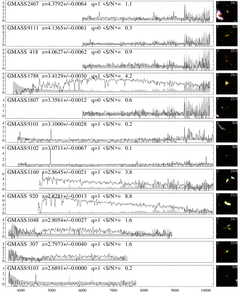
Figure 14: Spectra and postage stamp images of the 181 galaxies and stars with redshifts determined. Wavelength in Å on the horizontal axis and flux in $10^{-19}$ erg s^-1 Å^-1 cm^-2 on the vertical axis. Uncertainties caused by background noise are indicated by the underlying filled grey spectra. Indicated in each spectrum are: GMASS identification number, redshift and its uncertainty, redshift quality (1: secure, 0: tentative), and mean S/N per pixel. The postage stamps are constructed from HST/ACS observations in the $B$, $V$, and $I$ bands, convolved with a Gaussian kernel. Indicated are morphological class (see text, on the left) and $z$ magnitude (on the right). The spectra are sorted in descending order of redshift.

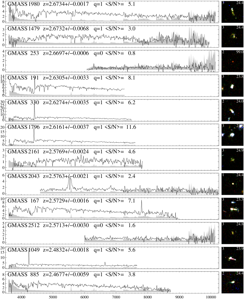
Figure 15: See Fig. 14 for description.

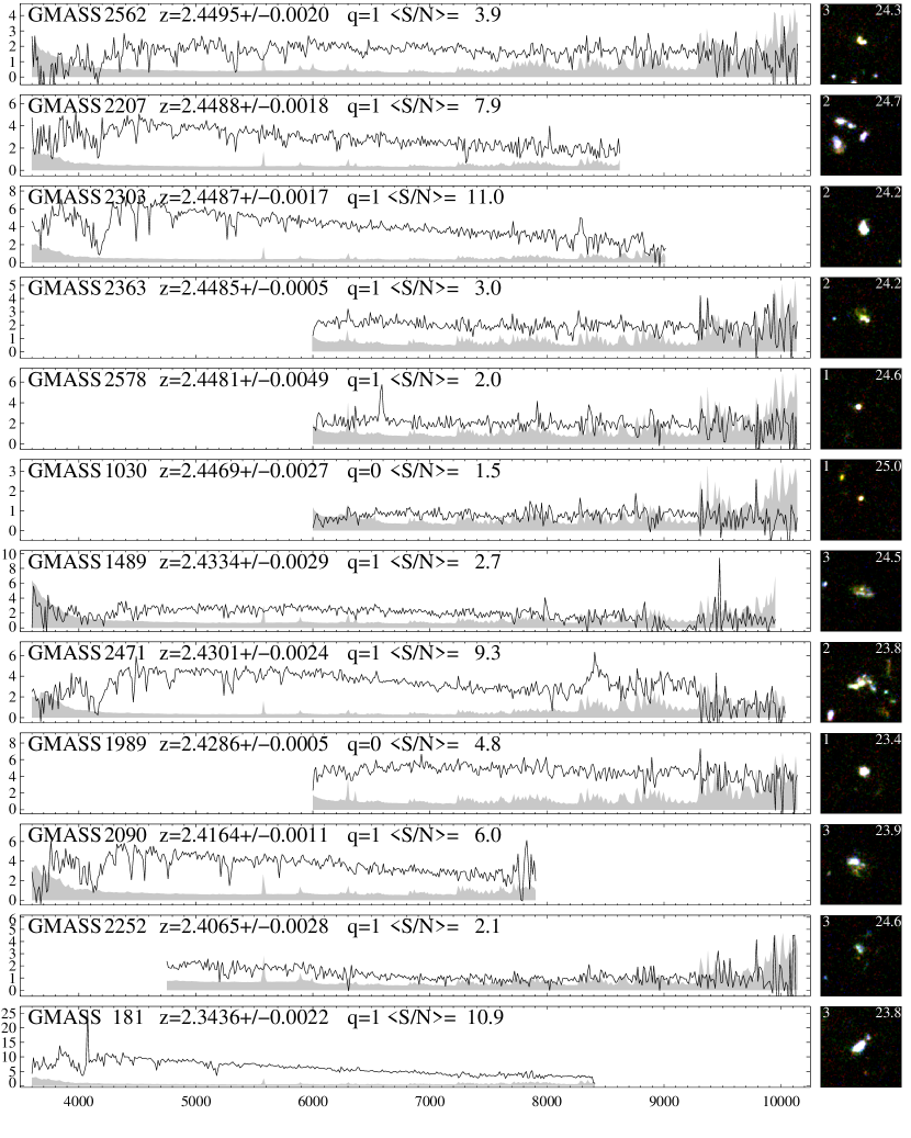
Figure 16: See Fig. 14 for description.

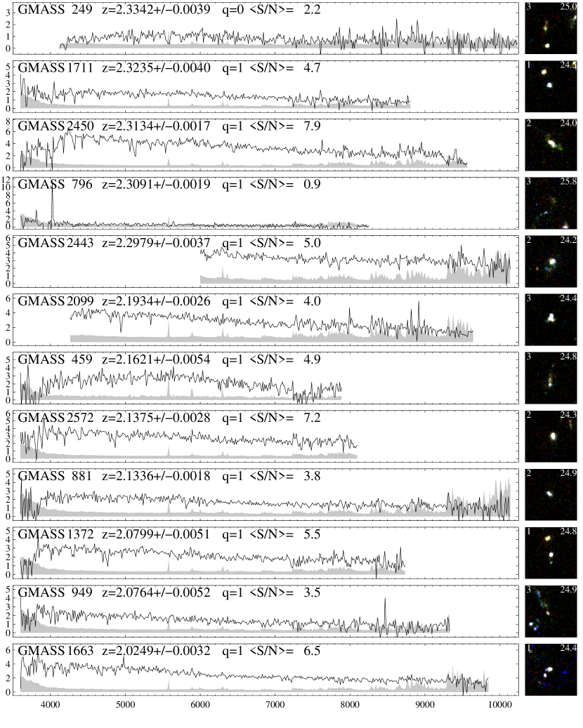
Figure 17: See Fig. 14 for description.

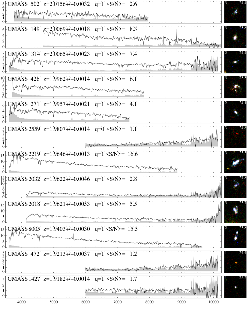
Figure 18: See Fig. 14 for description.

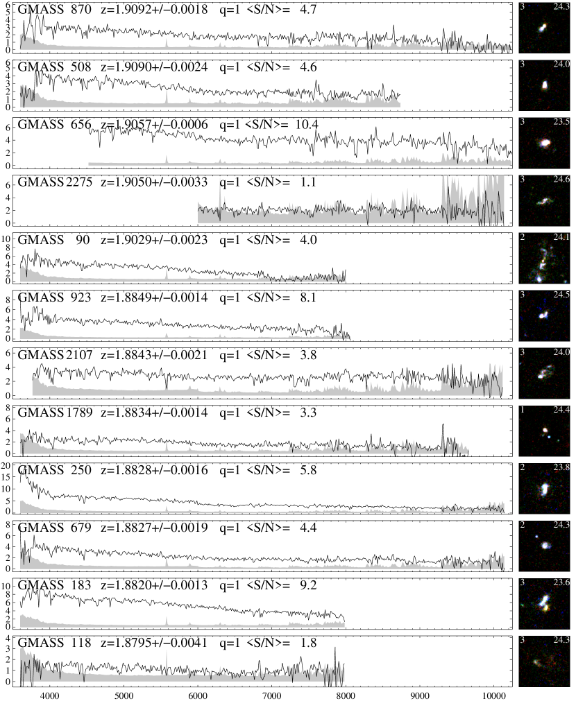
Figure 19: See Fig. 14 for description.

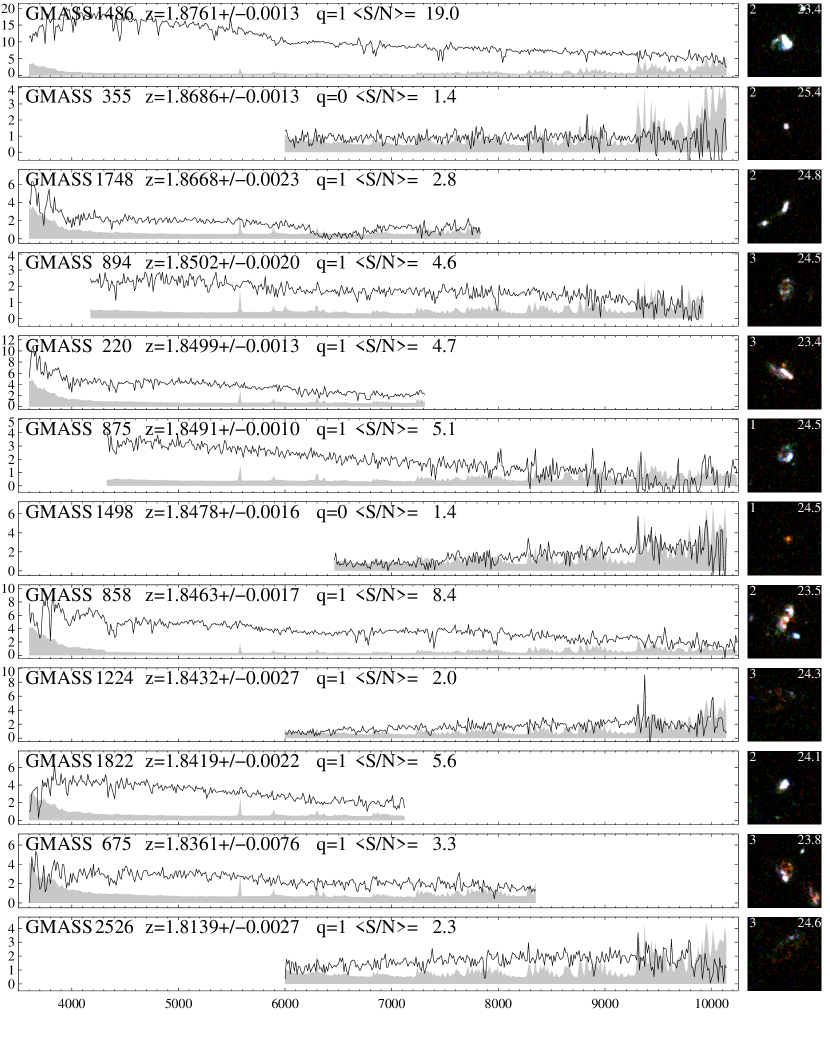
Figure 20: See Fig. 14 for description.

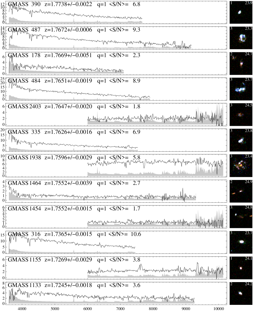
Figure 21: See Fig. 14 for description.

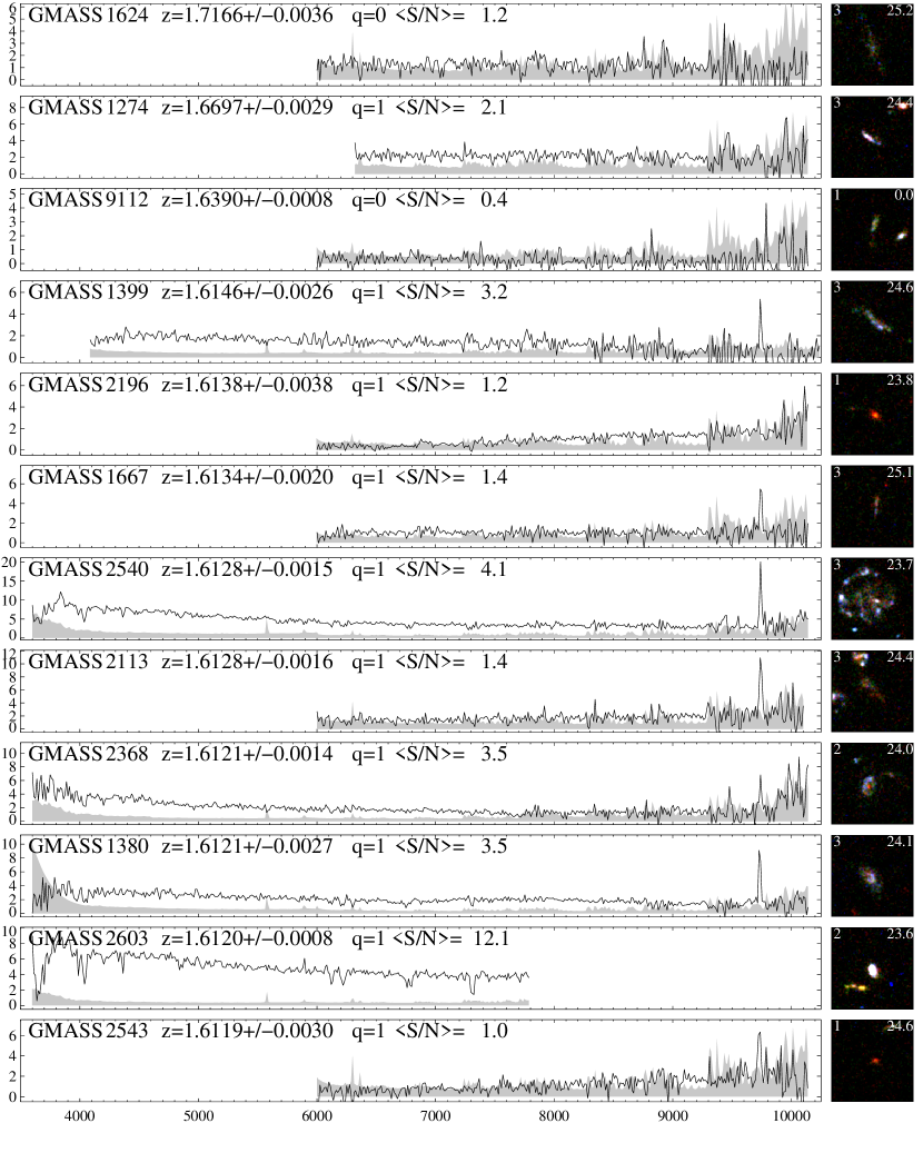
Figure 22: See Fig. 14 for description.

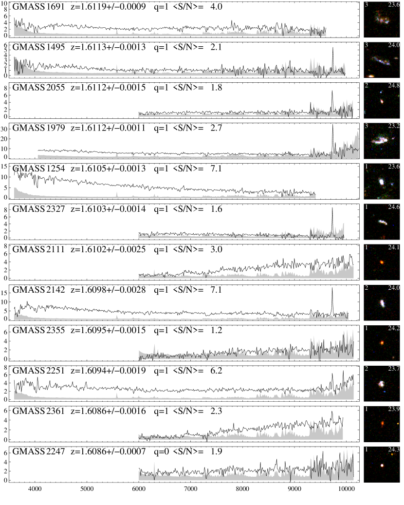
Figure 23: See Fig. 14 for description.

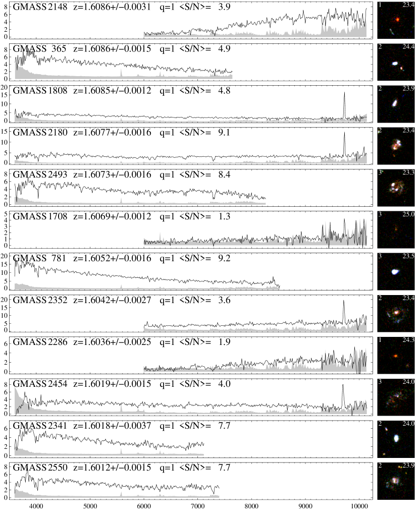
Figure 24: See Fig. 14 for description.

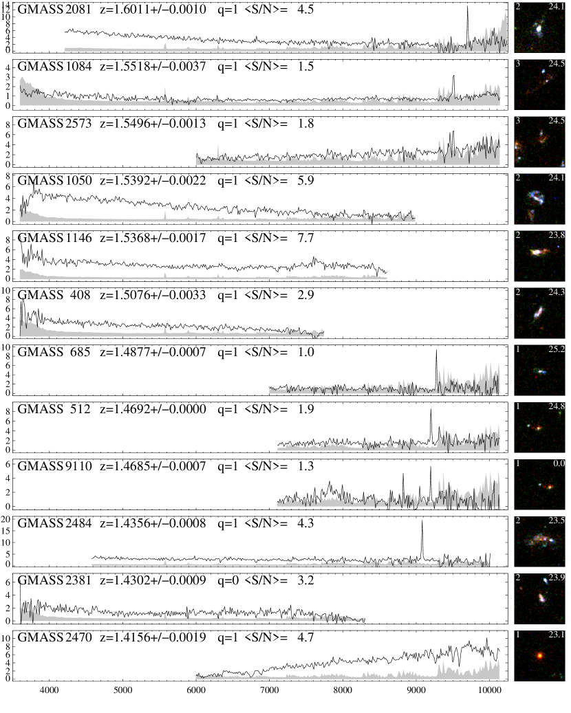
Figure 25: See Fig. 14 for description.

Figure 26: See Fig. 14 for description.

Figure 27: See Fig. 14 for description.

Figure 28: See Fig. 14 for description.

Figure 29: See Fig. 14 for description.

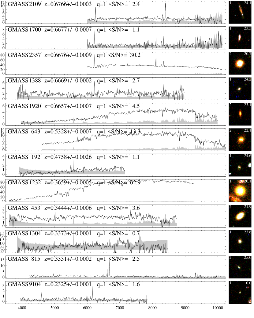
Figure 30: See Fig. 14 for description.

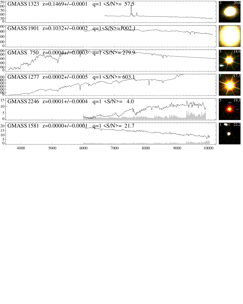
Figure 31: See Fig. 14 for description.