The molecular clump towards the eastern border of SNR G18.8+0.3

Abstract

Aims. The eastern border of the SNR G18.8+0.3, close to an HII regions complex, is a very interesting region to study the molecular gas that it is probably in contact with the SNR shock front.

Methods. We observed the aforementioned region using the Atacama Submillimeter Telescope Experiment (ASTE) in the ¹²CO J=3–2, ¹³CO J=3–2, HCO⁺ J=4–3, and CS J=7–6 lines with an angular resolution of 22^′′. To complement these observations, we analyzed IR, submillimeter and radio continuum archival data.

Results. In this work, we clearly show that the radio continuum “protrusion” that was early thought to belong to the SNR is an HII regions complex deeply embedded in a molecular clump. The new molecular observations reveal that this dense clump, belonging to an extended molecular cloud that surrounds the SNR southeast border, is not physically in contact with SNR G18.8+0.3, suggesting that the SNR shock front have not yet reached it or maybe they are located at different distances. We found some young stellar objects embedded in the molecular clump, suggesting that their formation should be approximately coeval with the SN explosion.

1 Introduction

The conversion of gas into stars involves a diversity of objects (molecular clouds, dust, magnetic fields, etc.) and several highly nonlinear and multidimensional dynamical processes (turbulence, self-gravity, etc.) operating at different scales, which are still far from understood in spite of all the theoretical and observational advances. Detailed multiwavelength studies at different spatial scales, from large clouds to star embryos, are very helpful to understand precisely how the gas and dust coalesces until forming new stars. Particularly, the investigation of the properties of the medium from which stars form, is a useful way to know the initial conditions that favour star formation and the most favourable mechanisms to trigger the process.

In this context, the molecular cloud suggested to be interacting with the SNR G18.8+0.3 (Dubner et al., 1999, 2004; Tian et al., 2007), which harbours IRAS pointlike sources compatible with the characteristics of protostellar candidates (IRAS sources whose colors correspond to those of ultracompact HII regions, i.e. sites of recent massive star formation, Wood & Churchwell (1989)) located very close to the SNR shock, is an interesting target. Its study allows us not only to analyze the properties of the interstellar matter around pre-stars, but also to explore if there exist some relation between the new born stars and the SNR. Studies of the molecular gas in regions suspected to be stellar nurseries, performed with intermediate spatial resolution, are especially useful to pinpoint the best candidates to pursue the millimetric and submillimetric studies with the unprecedented resources provided by ALMA.

The SNR G18.8+0.3 has a peculiar morphology with the eastern and southern flanks strongly flattened, while it fades to the west (Figure 1), suggesting a marked density gradient in the ambient gas. Based on VLA radio continuum observations, Dubner et al. (1996) pointed out the existence of a “protrusion” emerging from the eastern border of the SNR, near 18^h24^m14^s, -12^∘28^′30^′′(J2000). Subsequent observations performed with better angular resolution resolved, as described below, this region into several HII regions. In this paper, we analyze the molecular emission in this spot.

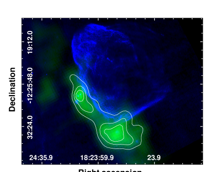
Figure 1: The SNR G18.8+0.3 radio continuum emission at 20 cm is displayed in blue and the ¹³CO J=1–0 emission, extracted from the GRS (Simon et al., 2001), which was averaged between 17 and 22 km s^-1 is presented in green with withe contours.

Arnal et al. (1993) early reported the detection of ¹²CO line emission along all the eastern border of the SNR G18.8+0.3, suggesting that the cloud might have been shocked by the expanding remnant. Later, Dubner et al. (1999) carried out observations in HI, ¹²CO and ¹³CO in the direction to G18.8+0.3, concluding that the SNR explosion took place near the border of a pre-existing cloud, driving a slow shock (v $\sim$ 10 km s^-1 ) into the cloud. Based on the systemic velocity v${}_{\rm{LSR}}\sim 19$ km s^-1 of the interacting molecular cloud, the distances of 1.9 and 14.1 kpc were estimated by applying a Galactic circular rotation model. In that paper, the distance ambiguity was wrongly interpreted favouring the closest option, a problem solved in Dubner et al. (2004), where the far distance of 14 kpc was confirmed for G18.8+0.3. More recently, based on ¹³CO emission and HI absorption techniques, Tian et al. (2007) established 6.9 kpc and 15 kpc as the lower and upper limits for the distance to this SNR.

2 Presentation of the investigated region

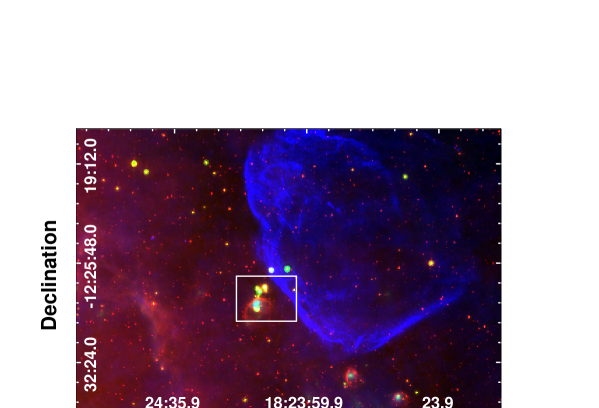
Figure 2: Three-color image of the SNR G18.8+0.3 and its surroundings. Again the radio continuum emission at 20 cm is presented in blue, the infrared bands at 8 $\mu$m and 24 $\mu$m are shown in red and green, respectively. The white rectangle shows the studied region.

Figure 1 shows the SNR G18.8+0.3 as seen in the radio continuum emission at 20 cm extracted from the MAGPIS (Helfand et al., 2006) (in blue) and its molecular environment in the ¹³CO J=1–0 emission averaged between 17 and 22 km s^-1 (in green). The ¹³CO data, with an angular resolution of 46^′′, were extracted from the Galactic Ring Survey (GRS; Simon et al. 2001). The image shows a clear large-scale morphological correspondence between the SNR southeastern border and the molecular gas, strongly suggesting an interaction between them, as was suggested in previous works. Figure 2 shows the SNR G18.8+0.3 radio continuum (again in blue) and its IR environment as seen in the Spitzer-IRAC band at 8 $\mu$m (red), and the Spitzer-MIPS band at 24 $\mu$m (green). The box indicates the region studied in this work. Figure 3 displays a zoom-in of this region showing the presence of several catalogued radio sources. The source RS1 is catalogued in the HII Region Discovery Survey (Anderson et al., 2011) as an irregular bubble (G18.751+0.254) with a recombination line at the LSR velocity 19.1 km s^-1, thus confirming that it is immersed in the same molecular cloud adjacent to the SNR G18.8+0.3. In Fig. 3, it can be appreciated the radio continuum emission of this HII region surrounded by 8 $\mu$m IR emission with a bright center emitting in 24 $\mu$m, as is usually observed in infrared dust bubbles (Churchwell et al., 2006, 2007). The sources RS2, RS3, and RS4, appear as discrete radio sources in the MAGPIS 20 cm Survey. In particular the source RS4, catalogued as a radio compact HII region (Giveon et al., 2005), lies at the same position as the 870 $\mu$m continuum source G18.76+0.26. This source, observed with the Large APEX Bolometer Camera (LABOCA) and catalogued in the ATLASGAL, has an angular extension of 59^′′$\times$42^′′ (Schuller et al., 2009). From observations of the NH₃ (1,1) line, these authors report a v${}_{\rm LSR}=20.8$ km s^-1 for G18.76+0.26, concluding that this source is located at the distance of about 14 kpc.

We conclude that the molecular complex abutting the eastern border of the SNR G18.8+0.3 is a very rich region populated by several HII regions. The HI absorption analysis performed by Tian et al. (2007) towards this region (region 6 in their work), gives an spectrum with the same absorption features as the spectra towards several regions over the SNR, strongly suggesting that this HII regions complex is located at the same distance as the SNR. Thus, we adopt a distance of about $14\pm 1$ kpc for the SNR, the molecular cloud and the HII regions complex. The error bar of 2 kpc comes by considering non-circular motions in the Galactic rotation model towards this region of the Galaxy.

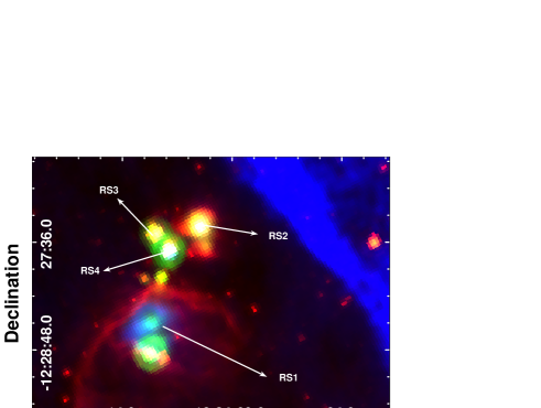
Figure 3: Three color image of the region marked with the white box in Fig. 2. Radio continuum at 20 cm = blue, 8 $\mu$m = red, and 24 $\mu$m = green. The catalogued radio sources described in the text are marked.

3 Observations

The molecular observations presented in this work were performed on June 12 and 13, 2011 with the 10 m Atacama Submillimeter Telescope Experiment (ASTE; Ezawa et al. 2004). We used the CATS345 GHz band receiver, which is a two-single band SIS receiver remotely tunable in the LO frequency range of 324-372 GHz. We simultaneously observed ¹²CO J=3–2 at 345.796 GHz and HCO⁺ J=4–3 at 356.734 GHz, mapping a region of 240^′′ $\times$ 150^′′ centered at RA $=$ 18^h24^m10.9^s, dec. $=-$12^∘28^′22.0^′′, J2000. We also observed ¹³CO J=3–2 at 330.588 GHz and CS J=7–6 at 342.883 GHz mapping a region of 120^′′ $\times$ 120^′′ centered at RA $=$ 18^h24^m10.9^s, dec. $=-$12^∘27^′20.0^′′. The mapping grid spacing was 20^′′ in all cases and the integration time was 30 and 60 sec per pointing in each case, respectively. All the observations were performed in position switching mode.

We used the XF digital spectrometer with a bandwidth and spectral resolution set to 128 MHz and 125 kHz, respectively. The velocity resolution was 0.11 km s^-1 and the half-power beamwidth (HPBW) was 22^′′ at 345 GHz. The weather conditions were optimal and the system temperature varied from T${}_{\rm sys}=150$ to 200 K. The main beam efficiency was $\eta_{\rm mb}\sim 0.65$. All quoted numbers for the line temperatures along this work were corrected for the antenna efficiency, i.e. in all cases they are the main brightness temperature. The spectra were Hanning smoothed to improve the signal-to-noise ratio and only linear or/and some third order polynomia were used for baseline fitting. The data were reduced with NEWSTAR and the spectra processed using the XSpec software package.

Figure 4: ¹²CO J=3–2 spectrum obtained towards the offset ($+$20^′′,$+$20^′′) position relative to RA $=$ 18^h24^m10.9^s, dec. $=-$12^∘28^′22.0^′′, J2000.

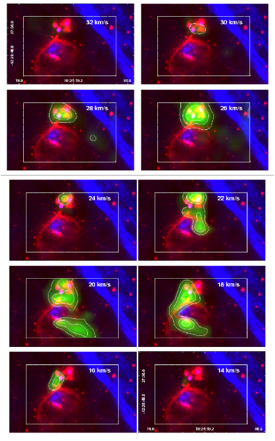
Figure 5: Integrated velocity channel maps of the ¹²CO J=3–2 emission every 2 km s^-1 (in green). As previous figures, in red is shown the IRAC emission at 8 $\mu$m and in blue the radio continuum emission at 20 cm. The contours levels in the upper panels (from 32 to 26 km s^-1) are 1.8, 3.6 and 7.0 K km s^-1, while the contours levels in the bottom panels (from 24 to 14 km s^-1) are 11.5, 15.0, and 19.5 K km s^-1. The dashed rectangle shows the mapped region.

4 Molecular gas

Figure 4 displays a typical ¹²CO J=3–2 spectrum obtained towards the surveyed region. This spectrum, corresponding to the offset position ($+$20^′′,$+$20^′′), exhibits two components: a weak one at $\sim$5 km s^-1, and the main component centered at $\sim 19$ km s^-1. The weak component corresponds to local gas emission and will not be further considered. The main component goes from $\sim$10 to 30 km s^-1, and represents the molecular gas that it is very likely related to the SNR and the HII regions complex. Figure 5 shows the gas distribution (in green) as seen in the ¹²CO J=3–2 emission integrated every 2 km s^-1 from 14 to 32 km s^-1. After integrating the ¹²CO J=3–2 emission from 10 to 30 km s^-1 we obtain the molecular clump shown in Fig. 6. The HII region G18.751+0.254 (source RS1 in Fig. 3, seen in blue in Fig. 4) appears surrounded by the molecular emission, whose peak coincides with the region where the sources RS2, RS3 and RS4 are located. Taking into account that the southeastern border of SNR G18.8+0.3 is surrounded by an extended molecular cloud detected in lower molecular transitions (see Fig. 1), we conclude that with the present observations we are analyzing a molecular clump belonging to this extended cloud.

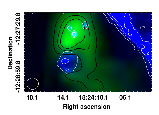
Figure 6: The ¹²CO J=3–2 emission integrated between 10 and 30 km s^-1 is presented in green with black contours with levels of 46, 65, and 80 K km s^-1. The radio continuum emission at 20 cm is shown in blue with white contours of 2.3, 6, and 11 mJy beam^-1. The angular resolutions are about 20^′′ and 6^′′ for the molecular and radio continuum emissions, respectively. The beam of the molecular observations is included towards the bottom left corner.

From the inspection of the other observed molecular transitions, we find that the HCO⁺ J=4–3 and ¹³CO J=3–2 lines are only bright near the peak of the molecular clump, i.e. towards the densest region. Figures 7 and 8 display the HCO⁺ J=4–3 and ¹³CO J=3–2 emissions, respectively, integrated between 10 and 30 km s^-1. In Fig. 8, the dashed yellow rectangle represents the region surveyed in the ¹³CO line.

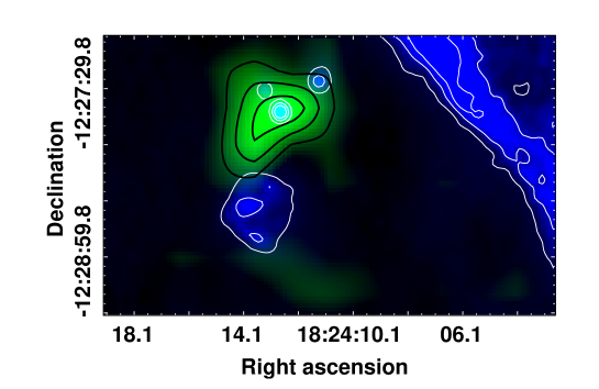
Figure 7: The HCO⁺ J=4–3 emission integrated between 10 and 30 km s^-1 is displayed in green with black contours with levels of 4, 6, and 8 K km s^-1. The radio continuum emission at 20 cm is shown in blue with white contours of 2.3, 6, and 11 mJy beam^-1.

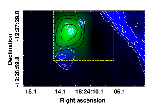
Figure 8: The ¹³CO J=3–2 emission integrated between 10 and 30 km s^-1 is presented in green with black contours with levels of 15, 20, and 30 K km s^-1. The radio continuum emission at 20 cm is shown in blue with white contours of 2.3, 6, and 11 mJy beam^-1. The dashed yellow rectangle represents the region surveyed in this line.

Based on the presented molecular maps we suggest that RS1 has shaped the surrounding gas, while the other radio sources, likely younger HII regions, are still embedded in the densest portion of the molecular clump. On the other hand it is important to note that the analyzed molecular clump is not in physical contact with the SNR G18.8+0.3 border, suggesting that the SNR shock front have not yet reached it or the clump is located at a different distance.

Figure 9 shows the spectra of each molecular species obtained towards the peak position of the molecular clump. The parameters determined from Gaussian fitting of these lines are presented in Table 1. T_mb represents the peak brightness temperature, V_LSR the central velocity referred to the Local Standard of Rest, and $\Delta$v is the FWHM line width. Errors are formal 1$\sigma$ value for the model of the Gaussian line shape. Additionally in this table are included the integrated intensities (I). It is noticeable that the HCO⁺ J=4–3 line appears significantly narrower than the CO lines, suggesting that the dense gas, mapped by the HCO⁺, occupies a different volume than the gas mapped by the ¹²CO and ¹³CO lines. Regarding the CS J=7–6 line, the data present some hints of emission towards this region. However the poor S/N ratio achieved in the observations of this transition does not allow us to perform a trustable analysis about this molecular species. The CS spectrum presented in Fig. 9, which was obtained towards the peak of the molecular clump, has a S/N ratio of about 2.2.

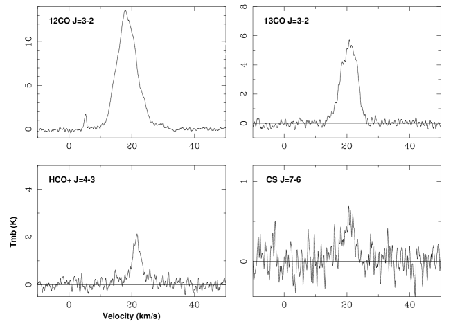
Figure 9: Spectra of each molecular species obtained towards the molecular clump peak. The ¹²CO, ¹³CO, and HCO⁺ lines have very high S/N ratio, while the CS emission has a S/N ratio of about 2.2.

Table 1: Observed and derived parameters of the molecular lines shown in Figure 9.

Emission	Tmb	VLSR	$\Delta$v	I
	(K)	(km s-1)	(km s-1)	(K km s-1)
12CO J=3–2	12.9 $\pm$0.1	18.5 $\pm$0.5	7.4 $\pm$0.1	104.7 $\pm$1.7
13CO J=3–2	5.5 $\pm$0.2	20.7 $\pm$0.5	6.0 $\pm$0.2	35.0 $\pm$1.8
HCO+ J=4–3	1.8 $\pm$0.3	21.5 $\pm$0.7	3.6 $\pm$0.5	9.0 $\pm$1.6

4.1 Column densities and abundances

To estimate the molecular column densities and abundances towards the clump we assume local thermodynamic equilibrium (LTE) and a beam filling factor of 1. From the peak temperature ratio between the CO isotopes (¹²T_mb/¹³T_mb), it is possible to estimate the optical depths from (e.g. Scoville et al. 1986):

$$\frac{{}^{12}{\rm T}_{mb}}{{}^{13}{\rm T}_{mb}}=\frac{1-exp(-\tau_{12})}{1-exp(-\tau_{12}/X)}$$ (1)

where $\tau_{12}$ is the optical depth of the ¹²CO gas and $X=$ [¹²CO]/[¹³CO] is the isotope abundance ratio. The [¹²CO]/[¹³CO] ratio can be estimated from the relation [¹²C]/[¹³C] $=6.21\times D_{G.C.}+18.77$ (Milam et al., 2005), where $D_{G.C.}=6.9$ kpc is the distance between the source and the Galactic Center, yielding [¹²C]/[¹³C] $=61\pm 14$. According to Milam et al. (2005) and Savage et al. (2002), the [¹²C]/[¹³C] isotope ratio exhibits a noticeable gradient with distance from the Galactic center, i.e. is strong dependent with $D_{G.C.}$. Then, from eq. 1, the ¹²CO J=3–2 optical depth is $\tau_{12}\sim 30$, while the ¹³CO J=3–2 optical depth is $\tau_{13}\sim 0.5$, revealing that the ¹²CO line appears optically thick, while the ¹³CO line is optically thin. Thus, we calculate the excitation temperature from

$$T_{ex}(3\rightarrow 2)=\frac{16.95{\rm K}}{{\rm ln}[1+16.59{\rm K}/(T_{\rm max}(^{12}{\rm CO})+0.036{\rm K})]}$$ (2)

obtaining $T_{ex}\sim 20$ K. Then, we derive the ¹²CO column density from:

$${\rm N(^{12}CO)}=7.96\times 10^{13}\leavevmode\nobreak\ e^{\frac{16.6}{T_{ex}}}\frac{T_{ex}+0.92}{1-exp(\frac{-16.6}{T_{ex}})}\int{\tau_{12}{\rm dv}}$$ (3)

where, taking into account that $\tau\geq 1$ we use the approximation:

$$\int{\tau\leavevmode\nobreak\ {\rm dv}}=\frac{1}{J(T_{ex})-J(T_{\rm BG})}\frac{\tau}{1-e^{-\tau}}\int{{\rm T_{mb}\leavevmode\nobreak\ dv}}$$ (4)

with

$$J(T)=\frac{h\nu/k}{exp(\frac{h\nu}{kT})-1}$$ (5)

Finally we obtain N(¹²CO) $\sim 1.5\times 10^{18}$ cm^-2. In the case of the ¹³CO J=3–2 line, we use:

$${\rm N(^{13}CO)}=8.28\times 10^{13}\leavevmode\nobreak\ e^{\frac{15.87}{T_{ex}}}\frac{T_{ex}+0.88}{1-exp(\frac{-15.87}{T_{ex}})}\int{\tau_{13}{\rm dv}}$$ (6)

and taking into account that this line appears optically thin, we use the approximation:

$$\int{\tau\leavevmode\nobreak\ {\rm dv}}=\frac{1}{J(T_{ex})-J(T_{\rm BG})}\int{{\rm T_{mb}\leavevmode\nobreak\ dv}}$$ (7)

yielding N(¹³CO) $\sim 1.8\times 10^{16}$ cm^-2.

The HCO⁺ column density was derived from:

$${\rm N(HCO^{+})}=5.85\times 10^{10}\leavevmode\nobreak\ e^{\frac{25.7}{T_{ex}}}\frac{T_{ex}+0.71}{1-exp(\frac{-17.12}{T_{ex}})}\int{\tau{\rm dv}}$$ (8)

and by assuming that the HCO⁺ J=4–3 is optically thin, we use the same approximation as used for the ¹³CO line (eq. 7). As excitation temperatures we use the range 20–50 K, obtaining N(HCO⁺) $\sim(3-5)\times 10^{12}$ cm^-2.

To estimate the molecular abundances it is necessary to have an H₂ column density value. As it will be shown in detail in the next section (Sect. 5), we independently estimate this parameter through the millimeter continuum emission, obtaining N(H₂) $\sim 4.4\times 10^{22}$ cm^-2. By using this value, we obtain the following molecular abundances: X(¹²CO) $\sim 3.4\times 10^{-5}$, X(¹³CO) $\sim 4.1\times 10^{-7}$, and X(HCO⁺) $\sim(0.7-1)\times 10^{-10}$. The obtained HCO⁺ abundance is very similar to the values derived by Cortes et al. (2010) and Cortes (2011) towards high-mass star-forming regions.

5 Millimeter continuum emission

We have also investigated the millimeter dust continuum emission at 1.1 mm using data from the Bolocam Galactic Plane Survey. We found a source in positional coincidence with the ¹²CO emission peak, BGPS 18.763+00.261 (Rosolowsky et al., 2010), which has a roughly elliptical morphology (41^′′$\times$29^′′). In Fig. 10, we present a two-color image of the BGPS 1.1 mm emission and the radio continuum emission at 20 cm. The positional agreement between the BGPS source and the molecular emission described above shows that the 1.1 mm emission originates in a densest portion of the molecular clump.

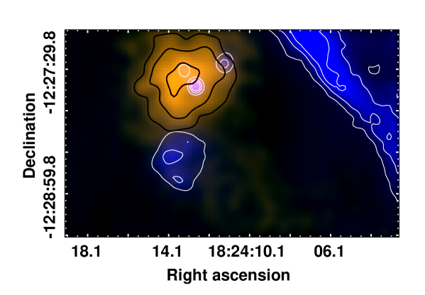
Figure 10: The smoothed 1.1 mm dust continuum emission is presented in orange with black contours. The radio continuum emission at 20 cm is shown in blue with white contours of 2.3, 6, and 11 mJy beam^-1.

We estimate the mass of the molecular gas associated with the BGPS source using the equations from Bally et al. (2010), M(H${}_{2})=14.26D^{2}S_{1.1}(e^{13/T_{d}}-1)M_{\odot}$, where $D$ is the distance in kpc, $S_{1.1}$ is the flux density at 1.1 mm in Jy, and $T_{d}$ is the dust temperature in K. Assuming that the dust and the gas are collisionally coupled, we can approximate $T_{d}=T_{K}$, where $T_{K}$ is the temperature of the gas. For $S_{1.1}$, we used the 80^′′ aperture flux density, which seems appropriate for the dimensions of this particular BGPS source. The flux value reported in Rosolowsky et al. (2010) was scaled with a calibration factor of 1.5 (Dunham et al., 2011). Thus, by adopting $D=14\pm 1$ kpc, $T_{d}=20$ K, and $S_{1.1}=2.21$ Jy we obtain M(H₂)$=5700\pm 800$ M_⊙. In addition, we estimated the column density of the molecular gas by applying N(H${}_{2})=2\times 10^{22}S_{1.1}$ cm^-2, obtaining N(H${}_{2})\sim 4.4\times 10^{22}$ cm^-2.

6 The compact radio sources embedded in the molecular gas

Figure 11 shows a three-color image (blue = radio continuum at 20 cm; green = 4.5 $\mu$m; red = 8 $\mu$m) of the studied region. The contours represent the ¹³CO J=3–2 emission integrated from 10 to 30 km s^-1 with levels of 15, 20, and 30 K km s^-1. The radio sources, RS2, RS3, and RS4 (see Section 2) are seen in projection onto the molecular gas condensation. The brightest one in the radio band, RS4, positionally coincides with the peak of the ¹³CO J=3–2 emission, while RS2 is located towards the northwestern border of the clump. From the figure it can be noticed that each radio source has 8 $\mu$m emission associated with an excellent spatial correlation, which confirms the thermal nature of the radio continuum emission. As noticed above, Giveon et al. (2005) identified RS4 as a young compact HII region. In this work we identify two new likely young HII regions, RS2 (G018.765+0.262) and RS3 (G018.762+0.270). While in the case of RS3 the radio continuum and the 8 $\mu$m emission have the same compact structure, in RS2 the 8 $\mu$m emission exhibits a shell-like structure that encircles the radio continuum emission.

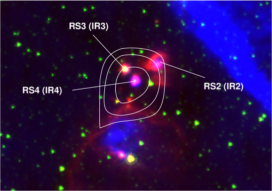
Figure 11: Three-color image (blue = radio continuum at 20 cm; green = 4.5 $\mu$m; red = 8 $\mu$m). The radio sources RS2, RS3, and RS4 are indicated, and between brackets it is indicated the nomenclature of the associated infrared sources: WISE J182411.60-122726.0 (IR2), J182413.49-122730.0 (IR3), and J182412.89-122742.2 (IR4). The contours represent the ¹³CO J=3–2 emission integrated between 10 and 30 km s^-1 with levels of 10, 15, and 30 K km s^-1.

From the WISE All-Sky Source Catalog (Wright et al., 2010) we searched for infrared sources related to radio ones. We identify the sources WISE J182411.60-122726.0 (IR2), J182413.49-122730.0 (IR3), and J182412.89-122742.2 (IR4), which are related to the radio sources RS2, RS3, and RS4, respectively.

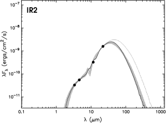
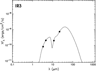
Figure 12: SED models for IR2, IR3, and IR4. The circles indicate the measured fluxes. Black and gray solid curves represent the best-fit model and the subsequent good fittings models (with $\chi^{2}-\chi^{2}_{best}<3$), respectively.

We performed a fitting of the spectral energy distribution (SED) of IR2, IR3, and IR4, using the tool developed by Robitaille et al. (2007) and adopting an interstellar extinction in the line of sight, $A_{v}$, between 14 and 50 magnitudes. The lower limit of $A_{v}$ was chosen by considering the typical value of one magnitude of absorption per kpc. The upper limit corresponds to that $A_{v}$ derived from the molecular material, estimated by using the relation $A_{v}=\frac{N(H_{2})}{0.94\times 10^{21}}$ mag (Frerking et al., 1982), with the N(H₂) derived in Sect. 5. In Figure 12 we show the SEDs for the three sources with the best-fitting model for each source (black curve) , and the subsequent good fitting models (grays curves) with $\chi^{2}-\chi^{2}_{best}<3$ (where $\chi^{2}_{best}$ is the $\chi^{2}$ per data point of the best-fitting model for each source). To construct the SED we consider the fluxes at the WISE 3.4, 4.6, 12, and 22 $\mu$m bands. Table LABEL:SEDpar presents the main physical parameters of each source as obtained from the best fitting model and the range from the subsequent models: star mass (Col. 2), star age (Col. 3), envelope accretion rate (Col. 4), bolometric luminosity (Col. 5), $\chi^{2}$ per data point of the best fitting model (Col. 6), and the number of subsequent good fitting models (Col. 7).

Table 2: Main physical parameters of IR2, IR3, and IR4 derived from the best fitting models for the SED of each source.

Source	$M_{\star}$		Age		$\dot{M}_{env}$		$L$		$\chi^{2}_{best}$	#models
	[M⊙]		[$\times 10^{5}$ yr]		[$\times 10^{-5}$ M⊙yr-1]		[$\times 10^{4}L_{\odot}$]			$\chi^{2}-\chi^{2}_{best}\leq 3$
	Best	Range	Best	Range	Best	Range	Best	Range
IR2	19	18-21	7	1-10	0	0-0.1	4	2-5	0.1	42
IR3	17	-	1	-	9.3	-	3	-	5.2	1
IR4	13	10-16	2	0.5-4	5.6	1-8	1	1-2	0.4	11

From the SED we conclude that the three sources are massive protostars. The derived ages are consistent with presence of ionized gas as detected in the radio continuum emission at 20 cm. It is well known that the formation of an ultracompact HII region around a massive protostar requires timescales about 10⁵ yr (Sridharan et al., 2002). The analysis of the SED also shows that IR2 seems to be the most evolved among the three sources. While IR3 and IR4 are protostars that are still accreting material at high rates ($\dot{M}_{env}>5\times 10^{-5}$ M_⊙yr^-1), IR2 probably finished its accretion stage ($\dot{M}_{env}\sim 0$). Moreover, from Fig. 11 it can be seen a shell-like morphology at 8 $\mu$m towards this source, which shows the border of an incipient photodissociation region. By comparing the age of these YSOs (see Table LABEL:SEDpar) with that of the SNR (about 10⁵ yrs), we conclude that the formation of the YSOs should be approximately coeval with the SN explosion, discarding the possibility that the SNR had triggered the star formation in the region. It it important to note that if the SED is performed using the near distances of 1–3 kpc, we obtain that the sources should be very young (ages of about $10^{4}$ yrs) with low masses (4-6 M_⊙); stellar sources with these parameters are unable to ionize the gas and generate an HII regions complex.

7 Concluding remarks

In this work we present the results from molecular observations (¹²CO and ¹³CO J=3–2, and HCO⁺ J=4–3) obtained with ASTE towards a molecular clump belonging to an extended cloud suggested to be interacting with the eastern flank of the SNR G18.8+0.3. Our observational study was complemented using IR, submillimeter and radio continuum data from public databases.

The surveyed region contains four radio sources, two of them catalogued as HII regions: G18.751+0.254 (RS1 in this work) and a compact one (RS4). The rest of the sources, IR2 and IR3, were identified as new young HII regions. We found a molecular clump, seen mainly in the ¹²CO J=3–2 line, partially surrounding the HII region G18.751+0.254 (RS1) with its densest portion located towards the north (seen at ¹³CO J=3–2 and HCO⁺ J=4–3). This densest portion coincides with the 1.1 mm continuum source BGPS 18.763+00.261, and the sources RS2, RS3, and RS4 are embedded in it.

The SNR G18.8+0.3 together with the radio sources RS1 and RS4, and the molecular gas have the same LSR velocity of about 20 km s^-1. We conclude that all the analyzed objects are located at the same distance of about $14\pm 1$ kpc. An important result is that the new molecular observations reveal that the surveyed molecular clump is not in physical contact with the SNR, suggesting that, either the SNR shock front have not yet reached the clump or they are located at different distances.

We identified the IR counterparts of the radio sources RS2, RS3, and RS4, those sources embedded in the densest portion of the molecular clump. From a SED fitting we conclude that they are YSOs of ages about 10⁵ yr, which is consistent with the presence of ionized gas as seen in the radio continuum emission at 20 cm. Their formation should be approximately coeval with the SN explosion, discarding triggered star formation by the action of the SNR.

References

- Anderson et al. (2011) Anderson, L. D., Bania, T. M., Balser, D. S., & Rood, R. T. 2011, ApJS, 194, 32
- Arnal et al. (1993) Arnal, E. M., Dubner, G., & Goss, W. M. 1993, Rev. Mexicana Astron. Astrofis., 26, 93
- Bally et al. (2010) Bally, J., Aguirre, J., Battersby, C., et al. 2010, ApJ, 721, 137
- Buckle et al. (2010) Buckle, J. V., Curtis, E. I., Roberts, J. F., & et al. 2010, MNRAS, 401, 204
- Churchwell et al. (2006) Churchwell, E., Povich, M. S., Allen, D., et al. 2006, ApJ, 649, 759
- Churchwell et al. (2007) Churchwell, E., Watson, D. F., Povich, M. S., et al. 2007, ApJ, 670, 428
- Cortes (2011) Cortes, P. C. 2011, ApJ, 743, 194
- Cortes et al. (2010) Cortes, P. C., Parra, R., Cortes, J. R., & Hardy, E. 2010, A&A, 519, A35
- Dubner et al. (1999) Dubner, G., Giacani, E., Reynoso, E., et al. 1999, AJ, 118, 930
- Dubner et al. (2004) Dubner, G., Giacani, E., Reynoso, E., & Parón, S. 2004, A&A, 426, 201
- Dubner et al. (1996) Dubner, G. M., Giacani, E. B., Goss, W. M., Moffett, D. A., & Holdaway, M. 1996, AJ, 111, 1304
- Dunham et al. (2011) Dunham, M. K., Rosolowsky, E., Evans, II, N. J., Cyganowski, C., & Urquhart, J. S. 2011, ApJ, 741, 110
- Ezawa et al. (2004) Ezawa, H., Kawabe, R., Kohno, K., & Yamamoto, S. 2004, in Presented at the Society of Photo-Optical Instrumentation Engineers (SPIE) Conference, Vol. 5489, Society of Photo-Optical Instrumentation Engineers (SPIE) Conference Series, ed. J. M. Oschmann, Jr., 763–772
- Frerking et al. (1982) Frerking, M. A., Langer, W. D., & Wilson, R. W. 1982, ApJ, 262, 590
- Giveon et al. (2005) Giveon, U., Becker, R. H., Helfand, D. J., & White, R. L. 2005, AJ, 129, 348
- Helfand et al. (2006) Helfand, D. J., Becker, R. H., White, R. L., Fallon, A., & Tuttle, S. 2006, AJ, 131, 2525
- Milam et al. (2005) Milam, S. N., Savage, C., Brewster, M. A., Ziurys, L. M., & Wyckoff, S. 2005, ApJ, 634, 1126
- Robitaille et al. (2007) Robitaille, T. P., Whitney, B. A., Indebetouw, R., & Wood, K. 2007, ApJS, 169, 328
- Rosolowsky et al. (2010) Rosolowsky, E., Dunham, M. K., Ginsburg, A., et al. 2010, ApJS, 188, 123
- Savage et al. (2002) Savage, C., Apponi, A. J., Ziurys, L. M., & Wyckoff, S. 2002, ApJ, 578, 211
- Schuller et al. (2009) Schuller, F., Menten, K. M., Contreras, Y., et al. 2009, A&A, 504, 415
- Scoville et al. (1986) Scoville, N. Z., Sargent, A. I., Sanders, D. B., et al. 1986, ApJ, 303, 416
- Simon et al. (2001) Simon, R., Jackson, J. M., Clemens, D. P., Bania, T. M., & Heyer, M. H. 2001, ApJ, 551, 747
- Sridharan et al. (2002) Sridharan, T. K., Beuther, H., Schilke, P., Menten, K. M., & Wyrowski, F. 2002, ApJ, 566, 931
- Tian et al. (2007) Tian, W. W., Leahy, D. A., & Wang, Q. D. 2007, A&A, 474, 541
- Wood & Churchwell (1989) Wood, D. O. S. & Churchwell, E. 1989, ApJ, 340, 265
- Wright et al. (2010) Wright, E. L., Eisenhardt, P. R. M., Mainzer, A. K., et al. 2010, AJ, 140, 1868