On some knot energies involving Menger curvature

Abstract

We investigate knot-theoretic properties of geometrically defined curvature energies such as integral Menger curvature. Elementary radii-functions, such as the circumradius of three points, generate a family of knot energies guaranteeing self-avoidance and a varying degree of higher regularity of finite energy curves. All of these energies turn out to be charge, minimizable in given isotopy classes, tight and strong. Almost all distinguish between knots and unknots, and some of them can be shown to be uniquely minimized by round circles. Bounds on the stick number and the average crossing number, some non-trivial global lower bounds, and unique minimization by circles upon compaction complete the picture.

Mathematics Subject Classification (2010): 49Q10, 53A04, 57M25

1 Introduction

In search of optimal representatives of given knot classes Fukuhara [23] proposed the concept of knot energies as functionals defined on the space of knots, providing infinite energy barriers between different knot types. This concept was made more precise later and was investigated by various authors; see e.g. [56], [12], [65], and we basically follow here the definition in the book of O’Hara [50, Definition 1.1].

Let $\mathcal{C}$ be the class of all closed rectifiable curves $\gamma\subset{\mathbb{R}}^{3}$ whose one-dimensional Hausdorff measure $\mathscr{H}^{1}(\gamma)$ is equal to 1. Moreover we assume that all curves in $\mathcal{C}$ contain a fixed point, say the origin in ${\mathbb{R}}^{3}$, and that all loops in $\mathcal{C}$ are parametrized by arclength defined on the interval $[0,1]$, i.e. $\gamma:[0,1]\to{\mathbb{R}}^{3}$ is Lipschitz continuous with $|\gamma^{\prime}|=1$ and $\gamma(0)=\gamma(1)$. Members of ${\mathcal{C}}$ will sometimes be referred to as (unit) loops.

Definition 1.1 (Knot energy).

Any functional $\mathscr{E}:{\mathcal{C}}\to[-\infty,\infty]$ that is finite on all simple smooth loops $\gamma\in{\mathcal{C}}$ with the property that $\mathscr{E}(\gamma_{i})$ tends to $+\infty$ as $i\to\infty$ on any sequence of simple loops $\gamma_{i}\in{\mathcal{C}}$ that converge uniformly to a limit curve with at least one self-intersection, is called self-repulsive or charge. If $\mathscr{E}$ is self-repulsive and bounded from below, it is called a knot energy.

One of the most prominent examples of a knot energy is the Möbius energy, introduced by O’Hara [47], and written here with a regularization slightly different from O’Hara’s [47, p. 243], and used, e.g., by Freedman, He, and Wang [22]:

$$\mathscr{E}_{\text{M\"{o}b}}(\gamma):=\int_{0}^{1}\int_{0}^{1}\left\{\frac{1}{|\gamma(s)-\gamma(t)|^{2}}-\frac{1}{d_{\gamma}(s,t)^{2}}\right\}\,ds\,dt\quad\,\,\,\text{for }\,\,\gamma\in{\mathcal{C}},$$

which is non-negative, since the intrinsic distance

$$d_{\gamma}(s,t):=\min\{|s-t|,1-|s-t|\}$$

of the two curve points $\gamma(s),\gamma(t)$ always dominates the extrinsic Euclidean distance $|\gamma(s)-\gamma(t)|.$ That this energy is indeed self-repulsive is proven in [49, Theorem 1.1] and [22, Lemma 1.2], and one is lead to the natural question if one can minimize $\mathscr{E}_{\text{M\"{o}b}}$ in a fixed knot class. In view of the direct method in the calculus of variations one would try to establish uniform bounds on minimizing sequences in appropriate norms to pass to a converging subsequence with limit hopefully in the same knot class.

However, O’Hara observed in [49, Theorem 3.1] that knots can pull tight in a convergent sequence of loops with uniformly bounded Möbius energy. This pull-tight phenomenon in a sequence of loops $\gamma_{i}\in{\mathcal{C}}$ is characterized by non-trivially knotted arcs $A_{i}\subset\gamma_{i}$ of a fixed knot type that are contained in open balls

$$B_{i}\equiv B_{r_{i}}(x_{i})\subset{\mathbb{R}}^{3},\quad\textnormal{such that $r_{i}\to 0$ as $i\to\infty;$}$$

see [50, Definition 1.3]. In principle this phenomenon could result in minimizing sequences for $\mathscr{E}_{\text{M\"{o}b}}$ of a fixed knot class, converging to a limit in a different knot class, and it is actually conjectured by Kusner and Sullivan [37] that this indeed happens. It was one of the great achievements of Freedman, He, and Wang in their seminal paper [22] to establish the existence of $\mathscr{E}_{\text{M\"{o}b}}$-minimizing knots but restricted to prime knot classes, with the help of the invariance of $\mathscr{E}_{\text{M\"{o}b}}$ under Möbius transformations.

Definition 1.2.

A knot energy $\mathscr{E}$ is minimizable if in each knot class there is at least one representative in ${\mathcal{C}}$ minimizing $\mathscr{E}$ within this knot class. $\mathscr{E}$ is called tight if $\mathscr{E}(\gamma_{i})$ tends to $+\infty$ on a sequence $\{\gamma_{i}\}\subset{\mathcal{C}}$ with a pull-tight phenomenon.

In that sense, $\mathscr{E}_{\text{M\"{o}b}}$ is conjectured to be not minimizable (on composite knots) since it fails to be tight. Changing the powers in the denominators, and allowing for powers of the integrand, there arises a whole family of different energies, and it depends on the ranges of parameters whether or not one finds minimizing knots; see [48, 49], [10].

The purpose of the present note is to investigate knot-energetic properties of geometrically defined curvature energies involving Menger curvature. The basic building block of these functionals are elementary geometric quantities like the circumcircle radius $R(x,y,z)$ of three distinct points $x,y,z\in{\mathbb{R}}^{3}$, the inverse of which is sometimes referred to as Menger curvature of $x,y,z$.

Varying one or several of the points $x,y,z$ along the curve $\gamma$ one obtains successive smaller radii, whose values then depend on the shape of the curve $\gamma$:

$$\varrho[\gamma](x,y):=\inf_{z\in\gamma\atop z\not=x\not=y\not=z}R(x,y,z),\quad\varrho_{G}[\gamma](x):=\inf_{y,z\in\gamma\atop z\not=x\not=y\not=z}R(x,y,z),\quad{\triangle}[\gamma]:=\inf_{x,y,z\in\gamma\atop z\not=x\not=y\not=z}R(x,y,z).$$ (1.1)

Repeated integrations over inverse powers of these radii with respect to the remaining variables lead to the various Menger curvature energies

$$\mathscr{M}_{p}(\gamma):=\int_{\gamma}\int_{\gamma}\int_{\gamma}\frac{d\mathscr{H}^{1}(x)d\mathscr{H}^{1}(y)d\mathscr{H}^{1}(z)}{R(x,y,z)^{p}},$$ (1.2)

$$\mathscr{I}_{p}(\gamma):=\int_{\gamma}\int_{\gamma}\frac{d\mathscr{H}^{1}(x)d\mathscr{H}^{1}(y)}{\varrho[\gamma](x,y)^{p}},$$ (1.3)

and

$${\mathscr{U}}_{p}(\gamma):=\int_{\gamma}\frac{d\mathscr{H}^{1}(x)}{\varrho_{G}[\gamma](x)^{p}},$$ (1.4)

where the integration is taken with respect to the one-dimensional Hausdorff-measure $\mathscr{H}^{1}$. By definition (1.1) of the radii the energy values on a fixed loop $\gamma\in{\mathcal{C}}$ are ordered as

$$\mathscr{M}_{p}(\gamma)\leq\mathscr{I}_{p}(\gamma)\leq{\mathscr{U}}_{p}(\gamma)\leq\frac{1}{\triangle[\gamma]^{p}}\,\,\,\text{for all }\,\,p\geq 1$$ (1.5)

with the limits

$$\lim_{p\to\infty}\mathscr{M}_{p}^{1/p}(\gamma)=\lim_{p\to\infty}\mathscr{I}_{p}^{1/p}(\gamma)=\lim_{p\to\infty}{\mathscr{U}}_{p}^{1/p}(\gamma)=\frac{1}{\triangle[\gamma]},$$ (1.6)

and each of the sequences $\{\mathscr{M}_{p}^{1/p}(\gamma)\}$, $\{\mathscr{I}_{p}^{1/p}(\gamma)\}$, $\{{\mathscr{U}}_{p}^{1/p}(\gamma)\}$ is non-decreasing as $p\to\infty$ on a fixed loop $\gamma\in{\mathcal{C}}.$

The idea of looking at minimal radii as in (1.1) goes back to Gonzalez and Maddocks [27], where $\varrho_{G}[\gamma]$ is introduced as the global radius of curvature of $\gamma$, and $\triangle$ stands for the thickness of the curve, which is justified by the fact that $\triangle$ equals the classic normal injectivity radius for smooth curves [27, Section 3]; see also [28, Lemma 3] for the justification in the non-smooth case. The quotient length/thickness (which equals $1/\triangle$ on the class ${\mathcal{C}}$ of unit loops) is called ropelength and plays a fundamental role in the search for ideal knots and links; see [28, Section 5], [16, Section 2], and [25]; see also [55] and [15]. Some knot-energetic properties of ropelength have been established (see e.g. [12, Theorems T4 and 4, Corollary 4.1]), and we are going to benefit from that.

Allowing higher order contact of circles (or spheres) to a given loop $\gamma\in{\mathcal{C}}$ one can define various other radii as discussed in detail in [26]. As a particular example we consider the tangent-point radius

$$r_{\textnormal{tp}}[\gamma](x,y)$$ (1.7)

as the radius of the unique circle through $x,y\in\gamma$ that is tangent to $\gamma$ at the point $x$, which, according to Rademacher’s theorem [19, Section 3.1, Theorem 1] on the differentiability of Lipschitz functions, is defined for almost every $x\in\gamma.$ This leads to the corresponding tangent-point and symmetrized tangent-point energy (as mentioned in [27, Section 6])

$$\mathscr{E}_{p}(\gamma):=\int_{\gamma}\int_{\gamma}\frac{d\mathscr{H}^{1}(x)d\mathscr{H}^{1}(y)}{r_{\textnormal{tp}}[\gamma](x,y)^{p}},\quad\mathscr{E}^{\textnormal{sym}}_{p}(\gamma):=\int_{\gamma}\int_{\gamma}\frac{d\mathscr{H}^{1}(x)d\mathscr{H}^{1}(y)}{\Big{(}r_{\textnormal{tp}}[\gamma](x,y)r_{\textnormal{tp}}[\gamma](y,x)\Big{)}^{p/2}}$$ (1.8)

to complement our list of Menger curvature energies on ${\mathcal{C}}$.

Remark 1.3.

In some of our earlier papers, see e.g. [54], [61], [57, 58], for technical reasons that are of no relevance here, parametric versions of (1.2)–(1.4) and (1.8) were considered. In the supercritical range of parameters that is considered throughout the present paper, finiteness of any of these curvature energies implies that $\gamma([0,1])\in{\mathcal{C}}$ is homeomorphic to a circle. Therefore, in virtually all the results below we assume, without any loss of generality, that $\gamma$ is a simple closed curve, i.e. $\gamma\colon[0,1)\to{\mathbb{R}}^{3}$ is injective and $\gamma(0)=\gamma(1)$.

Why do we care about these energies if there are already O’Hara’s potential energies such as $\mathscr{E}_{\text{M\"{o}b}}$, and – as a kind of hard or steric counterpart – ropelength? First of all, O’Hara’s energies require some sort of regularization due to the singularities of the integrands on the diagonal of the domain $[0,1]^{2}$, whereas the coalescent limit $x,y,z\to\zeta$ on a sufficiently smooth loop $\gamma$ leads to convergence of $1/R$ to classic curvature $\kappa_{\gamma}(\zeta)$:

$$\lim_{x,y,z\to\zeta}R^{-1}(x,y,z)=\kappa_{\gamma}(\zeta),$$

so that no regularization is necessary as pointed out by Banavar et al. in [3]. Moreover, using the elementary geometric definition of the respective integrands we have gained detailed insight in the regularizing effects of Menger curvature energies in a series of papers [61, 57, 58, 64, 32]. In particular, the uniform $C^{1,\alpha}$-a-priori estimates for supercritical values of the power $p$, that is, for $p$ above the respective critical value, for which the corresponding energy is scale-invariant, turn out to be the essential tool, not only for compactness arguments that play a central role in variational applications, but also in the present knot-theoretic context; see Section 2. Let us mention that even in the subcritical case these energies may exhibit regularizing behaviour if one starts on a lower level of regularity, e.g. with measurable sets [38],[39], [52, 53]. Integral Menger curvature $\mathscr{M}_{2}$, for example, plays a fundamental role in harmonic analysis for the solution of the Painlevé problem; see [43, 41, 67, 17, 66, 18]. Moreover, in contrast to O’Hara’s repulsive potentials, the elementary geometric integrands in (1.1) have lead to higher-dimensional analogues of discrete curvatures where one can establish similar $C^{1,\alpha}$-estimates for a priorily non-smooth admissible sets of finite energy of arbitrary dimension and co-dimension [59, 60, 62, 63, 33, 34, 35, 36], which could initiate further analysis of higher dimensional knot space. The problem of finding a higher-dimensional variant of, e.g., the Möbius energy that is analytically accessible to variational methods seems wide open; see [37, 2, 24]. Finally, recent work of Blatt and Kolasinski [7, 8],[9] characterizes the energy spaces of Menger-type curvatures in terms of (fractional) Sobolev spaces, so that one can hope to tackle evolution problems for integral Menger curvature $\mathscr{M}_{p}$, for instance, in order to untangle complicated configurations of the unknot, or to flow complicated representatives of a given knot class to a simpler configuration without leaving the knot class; see recent numerical work of Hermes in [30].

In order to investigate knot-energetic properties of the Menger curvature energies in (1.2)–(1.4) and (1.8) in more depth we will discuss three more properties (cf. [50, Definition 1.4]).

Definition 1.4.

1. A knot energy $\mathscr{E}$ on ${\mathcal{C}}$ is strong if there are only finitely many distinct knot types under each energy level.

2. A knot energy $\mathscr{E}$ distinguishes the unknot or is called unknot-detecting if the infimum of $\mathscr{E}$ over the trivial knots (the “unknots”) in ${\mathcal{C}}$ is strictly less than the infimum of $\mathscr{E}$ over the non-trivial knots in ${\mathcal{C}}$.

3. A knot energy $\mathscr{E}$ is called basic if the round circle is the unique minimizer of $\mathscr{E}$ in ${\mathcal{C}}.$

Many of the knot-energetic properties we establish here for Menger curvature energies can be summarized in the following table, where for comparison we have included the Möbius energy $\mathscr{E}_{\text{M\"{o}b}}$ and also total curvature

$$TK(\gamma):=\int_{\gamma}|\kappa_{\gamma}|\,ds\quad\textnormal{for sufficiently smooth loops $\gamma\in{\mathcal{C}}$,}$$ (1.9)

even though this energy as an integral over classic curvature, that is, over a purely local quantity, does not even detect self-intersections, so that total curvature fails to be a knot energy altogether.

Is the energy:	$\mathscr{M}_{p>3}$	$\mathscr{I}_{p>2}$	${\mathscr{U}}_{p>1}$	$\mathscr{E}_{p>2}$	$\mathscr{E}^{\textnormal{sym}}_{p>2}$	$1/\triangle$	$\mathscr{E}_{\text{M\"{o}b}}$	$TK$
charge	Yes	Yes	Yes	Yes	Yes	Yes	Yes	No
minimizable	Yes	Yes	Yes	Yes	Yes	Yes	No	No
tight	Yes	Yes	Yes	Yes	Yes	Yes	No	No
strong	Yes	Yes	Yes	Yes	Yes	Yes	Yes	No
unknot-detecting	?	Yes	Yes	Yes	Yes	Yes	Yes	Yes
basic	?	?	Yes	?	?	Yes	Yes	No

The respective index of each Menger curvature energy in this table denotes the admissible supercritical range of the power $p$, where we have neglected the fact that most of these energies do penalize self-intersections even in the scale-invariant case, that is, curves with double points have infinite energies $\mathscr{I}_{2}$, ${\mathscr{U}}_{1}$, $\mathscr{E}_{2}$; see [57, Proposition 2.1], [61, Lemma 1], and [64, Theorem 1.1].

Notice that the affirmative answers in the first five columns settle conjectures of Sullivan [65, p. 184] and O’Hara [50, p. 127] at least for the respective supercritical range of $p$ and for one-component links.

The Möbius energy $\mathscr{E}_{\text{M\"{o}b}}$ is strong since it bounds the average crossing number acn that according to [22, Section 3] can be written as

$$\text{acn}(\gamma):=\frac{1}{4\pi}\int_{0}^{1}\int_{0}^{1}\frac{|(\gamma^{\prime}(s)\times\gamma^{\prime}(t))\cdot(\gamma(t)-\gamma(s))|}{|\gamma(t)-\gamma(s)|^{3}}\,ds\,dt\quad\,\,\,\text{for }\,\,\gamma\in{\mathcal{C}},$$ (1.10)

where $\times$ denotes the usual cross-product in ${\mathbb{R}}^{3}.$ As a consequence of the good bound obtained in [22, Theorem 3.2] Freedman, He, and Wang can show that $\mathscr{E}_{\text{M\"{o}b}}$ also distinguishes the unknot; see [22, Corollary 3.4]. In [1] it is moreover shown that $\mathscr{E}_{\text{M\"{o}b}}$ is basic (as well as many other repulsive potentials), which settles the column for $\mathscr{E}_{\text{M\"{o}b}}$ in the table above. The only “Yes” for total curvature is due to the famous Farỳ-Milnor theorem [20], [45], which establishes the sharp lower bound $4\pi$ for the total curvature of non-trivially knotted loops, whereas the round circle has total curvature $2\pi$. Fenchel’s theorem ascertains the nontrivial lower bound $2\pi$ for $TK(\gamma)$ for any continuously differentiable loop $\gamma$ with equality if and only if $\gamma$ is a planar simple convex curve, which, however, does not suffice to single out the circle as the only minimizer, so $TK$ is not basic.

To justify the affirmative entries in the first four rows for the Menger curvature energies we are going to use compactness arguments based on the respective a priori estimates we obtained in our earlier work. This is carried out in Section 2. The properties “unknot-detecting” and “basic” are dealt with individually in Section 3, and there are some additional observations. The great circle on the boundary of a ball uniquely minimizes $\mathscr{I}_{p}$ for every $p\geq 2$ among all curves packed into that ball (Theorem 3.2). This restricted version of the property “basic” is accompanied by a non-trivial lower bound for $\mathscr{I}_{p}$ (Proposition 3.4), and the observation that $\gamma$ must be a circle if $R$, or $\varrho[\gamma]$, or $\varrho_{G}[\gamma]$ is constant along $\gamma$. In addition, we show that any minimizer of integral Menger curvature $\mathscr{M}_{p}$ is unknotted if $p$ is sufficiently large. In Section 4 we prove additional properties relevant for knot-theoretic considerations. In Theorem 4.1 we show that polygons inscribed in a loop of finite energy and with vertices spaced by some negative power of the energy value are isotopic to the curve. This produces a bound on the stick number (Corollary 4.2) and therefore also an alternative direct proof for these energies to be strong (Corollary 4.3); cf. [40, Theorem 2, Corollary 4] for related results for ropelength. Theorem 4.1 can also be used to prove that the energy level of two loops $\gamma_{1},\gamma_{2}\in{\mathcal{C}}$ determines a bound on the Hausdorff-distance $d_{\mathscr{H}}(\gamma_{1},\gamma_{2})$ below which the two curves are isotopic (Theorem 4.4). Both results rely on a type of excluded volume and restricted bending constraint that finite energy imposes on the curve, that we refer to as “diamond property” (see Definition 4.5), which is much weaker than positive reach [21]. It does not mean that there is a uniform neighbourhood guaranteeing the unique next-point projection, which would correspond to finite ropelength; see [28, Lemma 3]. Roughly speaking, it means that any chain of sufficiently densely spaced points carries along a “necklace” of diamond shaped regions as the only permitted zone for the curve within a larger tube; see Figure 2.

1.1 Open problems

The question marks in the table above depict unsolved problems. In particular the question if $\mathscr{M}_{p}$, $\mathscr{I}_{p}$, $\mathscr{E}_{p}$, or $\mathscr{E}_{p}^{\textnormal{sym}}$ are basic remains to be investigated. Notice, however, that Hermes recently proved that the circle is a critical point of $\mathscr{M}_{p}$ [30], which also supports our conjecture that all these energies are basic. Numerical experiments suggest that $\mathscr{M}_{p}$ should clearly distinguish the unknot, but so far we have not been able to prove that. Our bounds for the average crossing number acn are by far not good enough to capture that. Moreover, our compactness arguments to prove the properties in the first four rows of the table work in the respective supercritical case, i.e., for $p>3$ for $\mathscr{M}_{p}$, for $p>2$ for $\mathscr{I}_{p},\mathscr{E}_{p}$, and $\mathscr{E}_{p}^{\textnormal{sym}}$, and for $p>1$ for ${\mathscr{U}}_{p}$. But what happens for the geometrically interesting scale-invariant cases $\mathscr{M}_{3},\mathscr{I}_{2},\mathscr{E}_{2},\mathscr{E}_{2}^{\textnormal{sym}},{\mathscr{U}}_{1}$?

Further open problems include the regularity theory for minimizing knots of these energies (are they just $C^{1,\alpha}$, as all other curves of finite energy, or $C^{1,1}$, as the minimizers of the ropelength functional, cf. [16, Theorem 7] and [28, Theorem 4], or maybe $C^{\infty}$, like the minimizers of $\mathscr{E}_{\text{M\"{o}b}}$?), and better bounds — sharp for some knot families, if possible — for the average crossing number and stick number in terms of $\mathscr{M}_{p}$ and other energies, especially in the scale invariant cases mentioned above. Even partial answers would enlarge our knowledge of these curvature energies and their global properties.

Acknowledgement. The authors gratefully acknowledge: R. Ricca for organizing the ESF Conference on Knots and Links in Pisa in 2011, where parts of this work have been presented in progress; M. Giaquinta, for repeatedly hosting our stays at the Centro de Giorgi; and R. Kusner for creating the opportunity to finish this work at the Kavli Institute of Theoretical Physics (KITP) in Santa Barbara. This paper grew out of a larger project on geometric curvature energies financed, along with two workshops in Bȩdlewo and Steinfeld, by DFG and the Polish Ministry of Science. At KITP this research was supported in part by the National Science Foundation under Grant No. NSF PHY11-25915.

2 Charge, strong, and tight

We denote by $C^{0}([0,1])$ the space of continuous functions and recall the sup-norm

$$\|f\|_{C^{0}([0,1])}:=\sup_{s\in[0,1]}|f(s)|\quad\,\,\,\text{for }\,\,f\in C^{0}([0,1]),$$

and the Hölder seminorm

$$[f]_{0,\alpha}:=\sup_{s,t\in[0,1]\atop s\not=t}\frac{|f(s)-(t)|}{|s-t|^{\alpha}},$$

which together with the sup-norm constitutes the $C^{0,\alpha}$-norm

$$\|f\|_{C^{0,\alpha}([0,1])}:=\|f\|_{C^{0}([0,1])}+[f]_{0,\alpha}.$$

The higher order spaces $C^{k}([0,1])$, and $C^{k,\alpha}([0,1])$ consist of those functions that are $k$ times continuously differentiable on $[0,1]$ such that the sup-norm, respectively the sup-norm and the Hölder seminorm of the $k$-th derivative are finite.

Theorem 2.1.

Let $\mathscr{E}:{\mathcal{C}}\to(-\infty,\infty]$ be bounded from below such that

1. There exists $\delta=\delta(E)>0$, such that for all curves $\gamma\in{\mathcal{C}}$ with $\mathscr{E}(\gamma)<E$

   $$|\gamma(s)-\gamma(t)|>\min\big{\{}\delta,\frac{d_{\gamma}(s,t)}{2}\big{\}}.$$

2. $\mathscr{E}$ is sequentially lower semi-continuous on ${\mathcal{C}}\cap C^{1}([0,1],{\mathbb{R}}^{3})$ with respect to $C^{1}$-convergence.

3. There exist constants $C=C(E)$ and $\alpha=\alpha(E)\in(0,1]$ depending only on the energy level $E$ such that for all $\gamma\in{\mathcal{C}}$ with $\mathscr{E}(\gamma)\leq E$ one has $\gamma\in C^{1,\alpha}([0,1],{\mathbb{R}}^{3})$ with $\|\gamma\|_{C^{1,\alpha}([0,1],{\mathbb{R}}^{3})}\leq C.$

Then $\mathscr{E}$ is charge, minimizable, tight, and strong.

As an essential tool for the proof of this theorem let us recall that isotopy type is stable under $C^{1}$-convergence. In the $C^{2}$-category one finds this result, e.g., in Hirsch’s book [31, Chapter 8], whereas the only published proofs in $C^{1}$ we are aware of are in the papers by Reiter [51] and by Blatt in higher dimensions [6].

Theorem 2.2 (Isotopy).

For any curve $\gamma\in C^{1}([0,1],{\mathbb{R}}^{3})\cap{\mathcal{C}}$ there is $\epsilon_{\gamma}>0$ such that all closed curves $\beta\in C^{1}([0,1],{\mathbb{R}}^{3})$ with $\|\beta-\gamma\|_{C^{1}([0,1],{\mathbb{R}}^{3})}<\epsilon_{\gamma}$ are ambient isotopic to $\gamma.$

Proof of Theorem 2.1:  Assume that $\mathscr{E}$ is not charge, so that one finds a sequence of simple curves $\{\gamma_{i}\}\subset{\mathcal{C}}$ with uniformly bounded energy $\mathscr{E}(\gamma_{i})\leq E<\infty$, converging uniformly, that is, in the sup-norm to $\gamma$ which is not a simple loop. By assumption (i) there exist $\delta>0$ such that for all $i\in{\mathbb{N}}$ we have $|\gamma_{i}(s)-\gamma_{i}(t)|\geq\min\{\delta,d_{\gamma}(s,t)/2\}$. As $\gamma$ is not embedded, there exist $s\not=t\in[0,1)$ such that $\gamma(s)=\gamma(t)$ and for sufficiently large $i$ we have

$$\min\big{\{}\delta,\frac{d_{\gamma}(s,t)}{2}\big{\}}>|\gamma_{i}(s)-\gamma(s)|+|\gamma_{i}(t)-\gamma(t)|\geq|\gamma_{i}(s)-\gamma_{i}(t)|,$$

a contradiction. So, $\mathscr{E}$ is indeed charge.

Now we would like to minimize $\mathscr{E}$ on a given knot class $[K]$ within ${\mathcal{C}}$. Note first that by rescaling a smooth and regular representative of $[K]$ to length one and reparametrizing to arclength, we find that there is a representative of $[K]$ in ${\mathcal{C}}$. In particular, there is a minimal sequence $\{\gamma_{i}\}\subset{\mathcal{C}}$ with $\gamma_{i}\in[K]$ for all $i\in{\mathbb{N}}$, such that

$$\lim_{i\to\infty}\mathscr{E}(\gamma_{i})=\inf_{{\mathcal{C}}\cap[K]}\mathscr{E},$$

and the right-hand side is finite, since by assumption $\mathscr{E}$ is bounded from below. Thus the sequence of energy values $\mathscr{E}(\gamma_{i})$ is uniformly bounded by some constant $E\geq 0$ for all $i\in{\mathbb{N}}$ and by assumption (iii) there exist constants $C=C(E)$ and $\alpha=\alpha(E)\in(0,1]$ depending only on $E$ but not on $i\in{\mathbb{N}}$, such that

$$\|\gamma_{i}\|_{C^{1,\alpha}([0,1],{\mathbb{R}}^{3})}\leq C(E).$$

Thus, this sequence is equicontinuous, and by the theorem of Arzela-Ascoli we can extract a subsequence $\{\gamma_{i_{k}}\}\subset\{\gamma_{i}\}$ such that $\gamma_{i_{k}}$ converges to $\gamma$ in $C^{1}$, so that in particular $|\gamma^{\prime}|\equiv 1$. Assumption (i) implies that all $\gamma_{i_{k}}$ in the sequence are simple and, as $\mathscr{E}$ is charge, the limit curve is injective, hence

$$\mathscr{H}^{1}(\gamma)=\int_{0}^{1}|\gamma^{\prime}(s)|\,ds=\lim_{k\to\infty}\int_{0}^{1}|\gamma_{i_{k}}^{\prime}(s)|\,ds=\lim_{k\to\infty}\mathscr{H}^{1}(\gamma_{i_{k}})=1$$

because of the continuity of the length functional

$$\textnormal{length}(\gamma):=\int_{0}^{1}|\gamma^{\prime}(s)|\,ds$$

with respect to $C^{1}$-convergence. Therefore the limit curve $\gamma$ is in ${\mathcal{C}}\cap C^{1}([0,1],{\mathbb{R}}^{3}).$ We can use assumption (ii) to conclude

$$\mathscr{E}(\gamma)\leq\liminf_{k\to\infty}\mathscr{E}(\gamma_{i_{k}})=\inf_{{\mathcal{C}}\cap[K]}\mathscr{E}.$$

According to Theorem 2.2 we find that

$$[K]=[\gamma_{i_{k}}]=[\gamma]\quad\,\,\,\text{for all }\,\,k\gg 1,$$

so that $\gamma\in{\mathcal{C}}\cap[K]$ and therefore

$$\inf_{{\mathcal{C}}\cap[K]}\mathscr{E}\leq\mathscr{E}(\gamma)\leq\inf_{{\mathcal{C}}\cap[K]}\mathscr{E},$$

i.e. equality here, which establishes $\gamma\in{\mathcal{C}}$ as the (in general not unique) minimizer.

As to proving that $\mathscr{E}$ is tight we assume that there is a sequence with the pull-tight phenomenon with uniformly bounded energy. As above we find a $C^{1}$-convergent subsequence $\gamma_{i_{k}}$ with a $C^{1}$-limit curve $\gamma\in{\mathcal{C}}$ that necessarily has the same knot type as $\gamma_{i_{k}}$ for all sufficiently large $k$ according to Theorem 2.2. But this contradicts the fact that a subknot is pulled tight which would change the knot-type in the limit. Consequently, $\mathscr{E}$ is tight.

Assume finally that there are infinitely many knot-types $[K_{i}]$ with representatives $\gamma_{i}\in{\mathcal{C}}$ with uniformly bounded energy $\mathscr{E}(\gamma_{i})\leq E$ for all $i\in{\mathbb{N}}.$ Again, we extract a subsequence $\gamma_{i_{k}}\to\gamma$ in the $C^{1}$-topology. Hence $\mathscr{E}(\gamma)\leq E$ by assumption (ii), so that $\gamma$ is embedded by assumption (i). But then by means of Theorem 2.2 we reach a contradiction to infinitely many knot-types by $[\gamma]=[\gamma_{i_{k}}]$ for all sufficiently large $k\in{\mathbb{N}}.$ Consequently, $\mathscr{E}$ is also strong, which concludes the proof of the theorem. $\Box$

Corollary 2.3.

The energies $\mathscr{M}_{p}$ for $p>3$, $\mathscr{E}_{p}$, $\mathscr{E}^{\text{sym}}_{p}$, and $\mathscr{I}_{p}$ for $p>2$, and ${\mathscr{U}}_{p}$ for $p>1$ are charge, minimizable, tight, and strong.

Proof:    We need to check the validity of the assumptions in Theorem 2.1 for each of the energies under consideration.

For $\mathscr{I}_{p}$ assumption (i) follows from [57, Prop. 3.3], (ii) from [57, Lemma 3.5], and (iii) from Corollary 3.2 of [57].

For ${\mathscr{U}}_{p}$, assumption (ii) of Theorem 2.1 follows from [61, Thm. 3], (iii) of Theorem 2.1 is provided by [61, Thm. 1 (iv)], and to verify (i) one can use the results from Chapter 4 of the present paper, namely Lemma 4.6 and Proposition 4.7.

For integral Menger curvature $\mathscr{M}_{p}$ the situation is a little more subtle. By Theorem 1.4 in [58], if $\mathscr{M}_{p}(\gamma)<\infty$, then $\gamma([0,1])$ is, topologically, a segment or a circle. By the very definition of ${\mathcal{C}}$ for each $\gamma\in{\mathcal{C}}$ the first possibility can easily be excluded and we deal in fact with an arclength parametrized, simple closed curve $\gamma$. Thus, one can apply Theorems 1.2 and 4.3 in [58] to obtain the a priori estimate needed in (iii) along with (i), whereas (ii) is dealt with in Remark 4.5 of that paper.

To justify (i) for $\mathscr{E}_{p}$ we need to combine Theorem 1.1 in [64] with the aforementioned result of [58], which requires only one simple point of the locally homeomorphic curve to deduce injectivity of the arclength parametrization. (One simply has to copy the arguments in [58, Section 3.1] to extend the proof of Theorem 3.7 from that paper to cover the case of the tangent-point energy $\mathscr{E}_{p}$.) Uniform $C^{1,\alpha}$ bounds are given in Proposition 4.1 of [64]. With that information, the verification of lower semicontinuity of $\mathscr{E}_{p}$ on ${\mathcal{C}}\cap C^{1}$ is a simple exercise, requiring an application of Fatou’s lemma. Indeed, since

$$\frac{1}{r_{\text{tp}}(\gamma(t),\gamma(s))}=\frac{2\mathop{\rm dist}\nolimits(\gamma(s),\ell(t))}{|\gamma(t)-\gamma(s)|^{2}},$$

where $\ell(t)=\{\gamma(t)+\tau\gamma^{\prime}(t)\,\colon\,\tau\in{\mathbb{R}}\}$ is the tangent line to $\gamma$ at $\gamma(t)$, for curves $\gamma_{j}\to\gamma$ in $C^{1}$ we obviously have $1/r_{\text{tp}}(\gamma_{j}(t),\gamma_{j}(s))\to 1/r_{\text{tp}}(\gamma(t),\gamma(s))$ whenever the limit is nonzero, and the result follows.

As to $\mathscr{E}^{\text{sym}}_{p}$ we refer to Lemma 3.1.3 in [32], and in particular to the final estimate of its proof in [32, p. 23] to verify assumption (iii). Assumptions (i) and (ii) can be proven as we indicated above for $\mathscr{E}_{p}$. $\Box$

3 Basic, detecting unknots

Proposition 3.1.

The energy ${\mathscr{U}}_{p}$ is basic and unknot-detecting for all $p\geq 1$.

Proof:    We may assume ${\mathscr{U}}_{p}(\gamma)<\infty$, so that by [61, Theorem 1] $\gamma$ is in the Sobolev space $W^{2,1}$ of twice weakly differentiable functions with weak second derivatives in $L^{1}$. In particular, classic local curvature $\kappa_{\gamma}$ of $\gamma$ exists almost everywhere. Since $\varrho_{G}$ does not exceed the local radius of curvature wherever the latter exists [54, Lemma 7], we can estimate

$$4\pi\leq\int_{\gamma}|\kappa_{\gamma}|\,ds\leq\left(\int_{\gamma}|\kappa_{\gamma}|^{p}\,ds\right)^{1/p}\leq\left(\int_{\gamma}\big{(}{\varrho_{G}}[\gamma]\big{)}^{-p}\,ds\right)^{1/p}={\mathscr{U}}_{p}^{1/p}(\gamma)$$

for any non-trivially knotted curve $\gamma$ of length 1 by the Farý–Milnor theorem and Hölder’s inequality, whereas

$${\mathscr{U}}_{p}^{1/p}(\text{circle})=2\pi<4\pi\,.$$

Lemma 7 in [61] states that the circle uniquely minimizes ${\mathscr{U}}_{p}$. $\Box$

We do not know if the energies $\mathscr{M}_{p}$, $\mathscr{I}_{p},$ $\mathscr{E}_{p}$, and $\mathscr{E}^{\text{sym}}_{p}$ are basic or not. But for $\mathscr{I}_{p}$ we can at least prove a restricted version of that property, which may be interpreted as a relation between energy and compaction: When stuffing a unit loop into a closed ball the most energy efficient way (with respect to $\mathscr{I}_{p}$) is to form a great circle. Buck and Simon have established a non-trivial lower bound for their normal energy for curves packed into a ball in [12, Theorem 1], however, without presenting an explicit minimizer. It turns out that this normal energy is proportional to the tangent-point energy $\mathscr{E}_{2}$, and one might hope to use their bound for $\mathscr{I}_{2}$ by the simple ordering $\mathscr{I}_{2}\geq\mathscr{E}_{2}$ (cf. (3.16) in the proof of Corollary 3.7 below). But we obtain a better bound for $\mathscr{I}_{p}$ using a powerful sweeping argument which requires the infimum in the definition of the particular radius $\varrho[\gamma]$ in the integrand. Moreover, this technique of proof permits our uniqueness argument.

Theorem 3.2 (Optimal packing in ball).

Among all loops in ${\mathcal{C}}$ that are contained in a fixed closed ball $\overline{B_{\frac{1}{2\pi}}}$, circles of length $1$, i.e., great circles on $\partial B_{\frac{1}{2\pi}}$, “uniquely” minimize $\mathscr{I}_{p}$ for all $p\geq 2.$

We start with a technical lemma that also contains the aforementioned sweeping argument.

Lemma 3.3 (Sweeping).

Let $\gamma\subset{\mathcal{C}}$, and assume that there are two distinct points $x,y\in\gamma$ with

$$\rho:=\varrho[\gamma](x,y)>\frac{|x-y|}{2}.$$ (3.1)

Then no point of $\gamma$ is contained in the “sweep-out region”

$$S(x,y):=\bigcup_{x,y\in\partial B_{\rho}}B_{\rho}\setminus\overline{\bigcap_{x,y\in\partial B_{\rho}}B_{\rho}},$$ (3.2)

which is the union of all balls of radius $\rho$ containing $x$ and $y$ in their boundary $\partial B_{\rho}$ minus the closure of their intersection.

If, moreover, $|x-y|<\mathop{\rm diam}\nolimits\gamma$, or if the weaker assumption $|x-y|\leq|\xi-\eta|$ for at least one pair $(\xi,\eta)\in\gamma\times\gamma\setminus\{(x,y)\}$ holds, then $\gamma$ is not completely contained in the lens-shaped region

$$\ell(x,y):=\overline{\bigcap_{x,y\in\partial B_{\rho}}B_{\rho}},$$ (3.3)

and we have the estimate

$$1\geq|x-y|+\Big{(}2\pi-2\arcsin\frac{|x-y|}{2\rho}\Big{)}\rho,$$ (3.4)

in particular,

$$\rho\leq\frac{1}{\pi+2}.$$ (3.5)

Proof:    The first statement follows from elementary geometry.

 

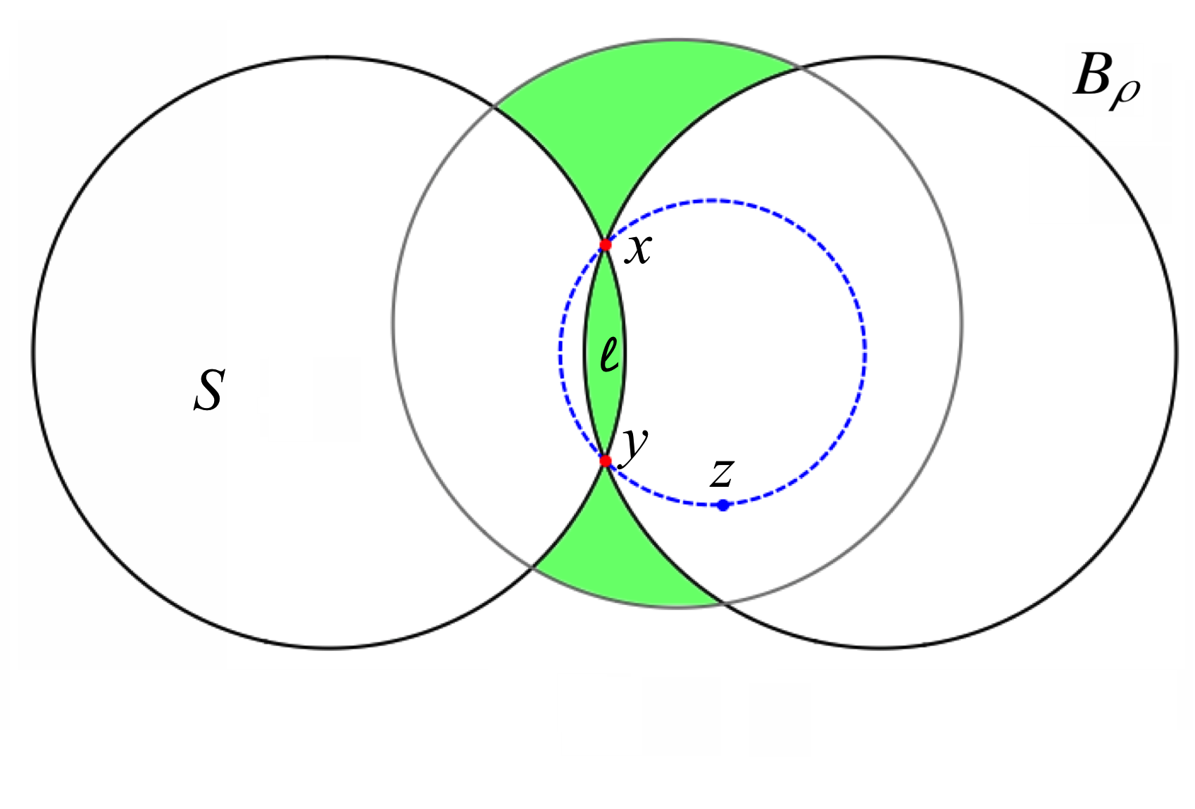
Figure 1: Left: If $x,y\in\gamma$ and $\varrho[\gamma](x,y)>|x-y|/2$, then $\gamma\cap S=\emptyset$ for a fairly large region $S=S(x,y)$. In the situation of Theorem 3.2 $\gamma$ is confined to the shaded zones. The solid circle in the middle depicts the boundary of the ball $B_{1/2\pi}$ containing $\gamma$. Right: A three-dimensional view of the sweep-out region $S$, whose boundary coincides with a self-intersecting torus of rotation, and of the ball $B_{1/2\pi}$, of which a substantial portion is immersed in that torus.

Indeed, if there were $z\in S(x,y)\cap\gamma$, then by elementary geometry carried out in the plane spanned by $x,y,$ and $z$, we would find

$$R(x,y,z)<\rho=\varrho[\gamma](x,y),$$

contradicting the very definition of $\varrho[\gamma](x,y)$; see the the dashed circle with radius $R(x,y,z)$ in the left image of Figure 1.

As to the second statement we use the weaker assumption and suppose to the contrary that $\gamma\subset\ell(x,y)$ which implies a direct contradiction via

$$\mathop{\rm diam}\nolimits\gamma=|x-y|>|\xi-\eta|\quad\,\,\,\text{for all }\,\,(\xi,\eta)\in\gamma\times\gamma\setminus\{(x,y)\}.$$

Next, observe that since $\gamma$ is a simple closed curve connecting $x$ and $y$, its unit length is bounded from below by the shortest possible simple loop connecting $x$ and $y$ without staying in $\ell(x,y)$ and without entering $S(x,y)$. Such a loop is the straight segment from $x$ to $y$ together with the circular great arc on the boundary of one of the balls $B_{\rho}$; hence (3.4) follows. The rough estimate (3.5) stems from comparing to the worst case scenario, when $x$ and $y$ are antipodal on a ball $B_{\rho}.$ $\Box$

Proof of Theorem 3.2.  We will simply say “circle” when we refer to a circle of unit length, i.e., a round circle in ${\mathcal{C}}$. It suffices to prove the statement for $p=2$, since

$$\mathscr{I}_{2}(\text{circle})<\mathscr{I}_{2}(\gamma)$$ (3.6)

for any $\gamma\in{\mathcal{C}}$ different from the circle implies by Hölder’s inequality

$$\mathscr{I}_{p}^{1/p}(\text{circle})=2\pi=\mathscr{I}_{2}^{1/2}(\text{circle})<\mathscr{I}_{2}^{1/2}(\gamma)\leq\mathscr{I}_{p}^{1/p}(\gamma)$$

for any $p>2.$

To show (3.6) we consider first the set $M^{+}(\gamma)$ of pairs of points $x,y\in\gamma$ such that

$$\varrho[\gamma](x,y)>\frac{1}{2\pi}=\frac{\mathop{\rm diam}\nolimits B_{\frac{1}{2\pi}}}{2}.$$ (3.7)

We shall prove that $M^{+}(\gamma)$ contains at most one such pair. If $M^{+}(\gamma)$ is empty, there is nothing to prove. Assume the contrary. Observe that $\varrho[\gamma](x,y)>|x-y|/2$ for each $(x,y)\in M^{+}(\gamma)$ since $\gamma\subset\overline{B_{\frac{1}{2\pi}}}$, and we can apply the first part of Lemma 3.3 to deduce that $\gamma$ has no point in common with the sweep-out region $S(x,y)$ defined in (3.2). Next, there can be at most one pair $(x,y)\in M^{+}(\gamma)$ such that $|x-y|=\mathop{\rm diam}\nolimits\gamma$, since $\gamma\cap S(x,y)=\emptyset$ and so $\gamma\subset\ell(x,y),$ which implies that $|\xi-\eta|<\mathop{\rm diam}\nolimits\gamma$ for all pairs $(\xi,\eta)\in\gamma\times\gamma$ different from $(x,y)$.

Now, fix $(x,y)\in M^{+}(\gamma)$ (with $|x-y|=\mathop{\rm diam}\nolimits\gamma$, if such a pair exists in $M^{+}(\gamma)$, and arbitrary otherwise). We claim that there cannot be any other point contained in $M^{+}(\gamma)$. Indeed, if there were $(u,w)\in M^{+}(\gamma)\setminus\{(x,y)\}$, then $|u-w|<\mathop{\rm diam}\nolimits\gamma$ and we could apply the second statement of Lemma 3.3 to the pair $(u,w)$ replacing $(x,y)$ to conclude that $\gamma\not\subset\ell(u,w)$. But then the simple curve $\gamma$ could not connect the points $u$ and $w$ and remain closed, since the complement $B_{\frac{1}{2\pi}}\setminus\big{(}S(u,w)\cup\ell(u,w)\big{)}$ is disconnected for each $(u,w)\in M^{+}(\gamma)$; see Figure 1, again with $(u,w)$ replacing $(x,y)$.

Thus, $M^{+}(\gamma)$ contains at most one pair of points. In other words,

$$\varrho[\gamma](\xi,\eta)\leq\frac{1}{2\pi}\quad\textnormal{for all $(\xi,\eta)\in\gamma\times\gamma\setminus(x,y)$,}$$ (3.8)

which immediately implies the energy inequality

$$\mathscr{I}_{2}^{1/2}(\gamma)\geq 2\pi=\mathscr{I}_{2}^{1/2}(\text{circle}).$$ (3.9)

To prove uniqueness of the minimizer we assume equality in (3.9), which implies by means of (3.8) that equality holds in (3.8) for almost all pairs $(\xi,\eta)\in\gamma\times\gamma.$ Now we claim that the set

$$M_{\textnormal{int}}(\gamma):=\{(\xi,\eta)\in\gamma\times\gamma:\varrho[\gamma](\xi,\eta)=\frac{1}{2\pi}\,\,\textnormal{ and $\xi$ or $\eta$ lie in the open ball $B_{\frac{1}{2\pi}}$}\}$$

contains at most one element. Indeed, for all pairs $(\xi,\eta)\in M_{\textnormal{int}}(\gamma)$ one has $\varrho[\gamma](\xi,\eta)>|\xi-\eta|/2$. Assuming that $M_{\textnormal{int}}(\gamma)$ has at least two elements we can select $(x,y),(\xi,\eta)$ in that set such that $|x-y|\leq|\xi-\eta|$ and apply Lemma 3.3 to obtain $\gamma\cap S(x,y)=\emptyset$ as well as $\gamma\not\subset\ell(x,y)$ which again implies a contradiction since $\gamma$ cannot connect $x$ and $y$ within $\overline{B_{\frac{1}{2\pi}}}$.

So we have shown that almost all $(\xi,\eta)\in\gamma\times\gamma$ satisfy equality in (3.8) and $\xi,\eta\in\partial B_{\frac{1}{2\pi}}(0)$. If there was any point $z\in\gamma\cap B_{\frac{1}{2\pi}}(0)$ then a whole subarc $\alpha\subset\gamma$ of positive length would lie in the open ball. Thus, $\alpha\times\alpha\subset M_{\textnormal{int}}(\gamma)$, contradicting the statement we just made. Hence $\gamma$ is completely contained in the boundary $\partial B_{\frac{1}{2\pi}}(0),$ and thus any three points $x,y,z\in\gamma$ must span an equatorial plane, otherwise $R(x,y,z)<1/(2\pi)$. But then there can be at most one such equatorial plane, which implies that $\gamma$ equals the great circle in that plane. $\Box$

The sweeping argument demonstrated in the proof of Theorem 3.2 can also be used to derive the following non-trivial lower bound, which states that one needs at least $\mathscr{I}_{2}$-energy level $16$ to close up a curve.

Proposition 3.4 (Lower bound for $\mathbf{\mathscr{I}_{p}}$).

For any loop $\gamma\in{\mathcal{C}}$ and $p\geq 2$ one has the energy estimate

$$\mathscr{I}_{p}^{1/p}(\gamma)\geq\mathscr{I}_{2}^{1/2}(\gamma)\geq\min\Big{\{}2+\pi,\frac{2}{\mathop{\rm diam}\nolimits\gamma}\Big{\}}\geq 4.$$ (3.10)

Proof:    The first inequality is just Hölder’s inequality, the last can be seen directly, since the diameter of $\gamma$ is bounded by half of its length. The second inequality in (3.10), however, requires a proof.

First we claim that there is a set $T\subset\gamma\times\gamma$ of positive measure such that for each pair of points $(x,y)\in T$ one has

$$\frac{1}{\varrho[\gamma](x,y)^{2}}\leq\mathscr{I}_{2}(\gamma),$$ (3.11)

since otherwise we could integrate the reverse inequality to get the contradictory statement

$$\mathscr{I}_{2}(\gamma)=\int_{\gamma}\int_{\gamma}\frac{d\mathscr{H}^{1}(\xi)d\mathscr{H}^{1}(\eta)}{\varrho[\gamma](\xi,\eta)^{2}}>\mathscr{I}_{2}(\gamma).$$

If one pair $(x,y)\in T$ satisfies $\varrho[\gamma](x,y)=|x-y|/2$ which is bounded from above by $\mathop{\rm diam}\nolimits\gamma/2$, then we obtain from (3.11)

$$\frac{1}{\mathscr{I}_{2}^{1/2}(\gamma)}\leq\varrho[\gamma](x,y)\leq\frac{\mathop{\rm diam}\nolimits\gamma}{2},$$

which gives the second alternative of the minimum in (3.10).

In the other case, $\varrho[\gamma](x,y)>|x-y|/2$ for all $(x,y)\in T$, and we can apply Lemma 3.3 again since we can pick two pairs $(x,y),(\xi,\eta)\in T$ with $|x-y|\leq|\xi-\eta|$. This results in $\gamma\cap S=\emptyset$ and $\gamma\not\subset\ell(x,y)$, where $S$ and $\ell$ are defined in (3.2) and (3.3), respectively. Then we insert the rough estimate (3.5) into (3.11) to obtain the remaining alternative in the desired estimate (3.10). $\Box$

As another immediate consequence of the sweeping technique we observe that constant $R$, $\varrho[\gamma]$, or $\varrho_{G}[\gamma]$ allows only for the circle. Recall that constant classic local curvature does not imply anything like that; see, e.g. the construction of arbitrary $C^{2}$-knots of constant curvature in [42].

Corollary 3.5 (Rigidity).

If there is $R_{0}\in(0,\infty)$, such that a curve $\gamma\in{\mathcal{C}}$ satisfies either $R(x,y,z)\equiv R_{0}$, or $\varrho[\gamma](x,y)\equiv R_{0}$, or $\varrho_{G}[\gamma](x)\equiv R_{0}$ for all $x,y,z\in\gamma$, then $R_{0}=1/(2\pi)$ and $\gamma$ is the round circle of radius $1/(2\pi)$.

Proof:    By definition (1.1) of the respective radii it suffices to prove the statement under the assumption that $\varrho_{G}[\gamma](x)=R_{0}$ for all $x\in\gamma.$ Notice first that this implies $1/\triangle[\gamma]=1/R_{0}<\infty$ such that by [28, Lemmata 1 & 2] $\gamma$ is simple and of class $C^{1,1}([0,1],{\mathbb{R}}^{3})$. Moreover, by the elementary geometric expression for $R$ one finds $\mathop{\rm diam}\nolimits\gamma\leq 2R_{0}$.

We claim that, in fact, $\mathop{\rm diam}\nolimits\gamma=2R_{0}$, since if not, we could find points $x,y\in\gamma$ with

$$\mathop{\rm diam}\nolimits\gamma=|x-y|<2R_{0}=2\varrho_{G}[\gamma](x),$$

and we deduce from the first part of Lemma 3.3 that $S(x,y)\cap\gamma=\emptyset$, where $S(x,y)$ is the sweep-out region defined in (3.2) for $\rho:=\varrho_{G}[\gamma](x)=R_{0}\leq\varrho[\gamma](x,y).$ Since $x$ and $y$ realize the diameter of $\gamma$ we conclude that $\gamma$ is completely contained in the lens-shaped region $\ell(x,y)$ defined in (3.3) for $\rho=\varrho_{G}[\gamma](x),$ which immediately gives a contradiction, since $\gamma$ is of class $C^{1}$ and can therefore have no corner points at $x$ and $y$. This proves $\mathop{\rm diam}\nolimits\gamma=2R_{0}$, so that $\gamma$ is contained in the closure of the ball $B^{*}:=B_{R_{0}}(\frac{x+y}{2})$, since any point on $\gamma$ but outside the closed slab of width $|x-y|$ and orthogonal to the segment $x-y$ would lead to a larger diameter, and any point $\zeta\in\gamma\setminus\overline{B^{*}}$ inside the slab would lead to the contradiction $R(x,y,\zeta)<R_{0}=\varrho_{G}[\gamma](x).$ But with $\gamma\subset\overline{B^{*}}$ we can apply our best packing result, Theorem 3.2, to conclude that $\gamma$ must coincide with a great circle on the boundary $\partial B^{*}$ because of the identity

$$\frac{1}{R_{0}}=\mathscr{I}_{2}^{1/2}(\gamma)=\mathscr{I}_{2}^{1/2}(\textnormal{great circle on $\partial B^{*}$})=\frac{1}{R_{0}}.$$

Since $\gamma\in{\mathcal{C}}$ has length one, we compute $R_{0}=1/(2\pi).$ $\Box$

The energies $\mathscr{I}_{p}$, $\mathscr{E}_{p}$ and $\mathscr{E}_{p}^{\text{sym}}$ for $p\geq 2$ are also unknot-detecting. This follows via simple applications of Hölder and Young inequalities from a key ingredient which is an inequality, due to Simon and Buck, cf. [12, Theorem 3], between $\mathscr{E}_{2}^{\text{sym}}$ and the average crossing number, defined in (1.10).

Here is the result, for which we present here a short proof for the sake of completeness.

Theorem 3.6 (Buck, Simon).

Let $\gamma\in{\mathcal{C}}$ be a simple curve of class $C^{1}$. Then

$$\mathscr{E}_{2}^{\text{\rm sym}}(\gamma)\geq 16\pi\,\text{\rm acn}\,(\gamma).$$ (3.12)

Proof:    The theorem follows from a pointwise inequality between the integrands. To see that, let $s\not=t\in[0,1]$ and $r(s,t)=\frac{\gamma(s)-\gamma(t)}{|\gamma(s)-\gamma(t)|}$. Set

$$\alpha=\alpha(s,t)=\mathop{\mbox{$<\!\!\!)$}}\nolimits\big{(}\gamma^{\prime}(s),r(s,t)\big{)}\,,\qquad\beta=\beta(s,t)=\mathop{\mbox{$<\!\!\!)$}}\nolimits\big{(}\gamma^{\prime}(t),r(s,t)\big{)}\,,$$

and rewrite (1.10) as

$$\text{acn}\,(\gamma)=\frac{1}{4\pi}\iint_{[0,1]\times[0,1]}\frac{\big{|}\det(\gamma^{\prime}(s),\gamma^{\prime}(t),r(s,t))\big{|}}{|\gamma(s)-\gamma(t)|^{2}}\;ds\,dt.$$ (3.13)

We have

$$\big{|}\det(\gamma^{\prime}(s),\gamma^{\prime}(t),r(s,t))\big{|}=|\gamma^{\prime}(s)\times r(s,t)|\cdot\mathop{\rm dist}\nolimits\big{(}\gamma^{\prime}(t),\text{span}(\gamma^{\prime}(s),r(s,t))\big{)}=\sin\alpha\cdot\sin\varphi,$$

where $\varphi=\varphi(s,t)$ denotes the angle between $\gamma^{\prime}(t)$ and $\text{span}(\gamma^{\prime}(s),r(s,t))$. Denoting the orthogonal projection of ${\mathbb{R}}^{3}$ onto $P:=\text{span}(\gamma^{\prime}(s),r(s,t))$ by $\pi$, one clearly obtains

$$\sin\varphi=|\gamma^{\prime}(t)-\pi(\gamma^{\prime}(t))|=\mathop{\rm dist}\nolimits\big{(}\gamma^{\prime}(t),P\big{)}\leq\big{|}\gamma^{\prime}(t)-\langle\gamma^{\prime}(t),r(s,t)\rangle\,r(s,t)\big{|}=\sin\beta.$$

Thus,

$$\frac{\sin\alpha(s,t)\;\sin\beta(s,t)}{|\gamma(s)-\gamma(t)|^{2}}\geq\frac{\big{|}\det(\gamma^{\prime}(s),\gamma^{\prime}(t),r(s,t))\big{|}}{|\gamma(s)-\gamma(t)|^{2}}\,.$$ (3.14)

The left–hand side above is directly related to the tangent–point radius, as a simple geometric argument shows that

$$\frac{1}{r_{\textnormal{tp}}[\gamma](\gamma(s),\gamma(t))}=\frac{2\mathop{\rm dist}\nolimits(\gamma(t),\gamma(s)+\text{span}\,\gamma^{\prime}(s))}{|\gamma(s)-\gamma(t)|^{2}}=\frac{2\sin\alpha(s,t)}{|\gamma(s)-\gamma(t)|}\,.$$

Hence, (3.14) translates to

$$\frac{1}{r_{\textnormal{tp}}[\gamma](\gamma(s),\gamma(t))}\cdot\frac{1}{r_{\textnormal{tp}}[\gamma](\gamma(t),\gamma(s))}\geq 4\frac{\big{|}\det(\gamma^{\prime}(s),\gamma^{\prime}(t),r(s,t))\big{|}}{|\gamma(s)-\gamma(t)|^{2}}\,.$$

Integrating, we obtain (3.12). $\Box$

Corollary 3.7 (Unknot-detecting).

The energies $\mathscr{I}_{p}$, $\mathscr{E}_{p}$ and $\mathscr{E}_{p}^{\text{sym}}$ are unknot-detecting for each $p\geq 2$.

Proof:    By Hölder’s inequality, for curves of unit length we have

$$\mathscr{F}_{p}(\gamma)^{2/p}\geq\mathscr{F}_{2}(\gamma),\qquad p\geq 2,$$ (3.15)

for each energy $\mathscr{F}_{p}\in\{\mathscr{E}_{p},\mathscr{E}_{p}^{\text{sym}},\mathscr{I}_{p}\}$. Besides,

$$\mathscr{I}_{2}\geq\mathscr{E}_{2}\geq\mathscr{E}_{2}^{\text{sym}}.$$ (3.16)

To verify the second inequality in (3.16), just note

$$\frac{1}{2}\biggl{(}\frac{1}{r_{\textnormal{tp}}[\gamma](\gamma(s),\gamma(t))^{2}}+\frac{1}{r_{\textnormal{tp}}[\gamma](\gamma(t),\gamma(s))^{2}}\biggr{)}\geq\frac{1}{r_{\textnormal{tp}}[\gamma](\gamma(s),\gamma(t))}\cdot\frac{1}{r_{\textnormal{tp}}[\gamma](\gamma(t),\gamma(s))}$$

and integrate both sides with respect to $(s,t)\in[0,1]^{2}$.

In order to check that $\mathscr{I}_{2}\geq\mathscr{E}_{2}$ we use the explicit formula for the tangent-point radius from elementary geometry

$$r_{\textnormal{tp}}[\gamma](x,y)=\frac{|x-y|}{2\sin\mathop{\mbox{$<\!\!\!)$}}\nolimits(y-x,t_{x})},$$

where we assumed that the unit tangent $t_{x}$ of $\gamma$ at the point $x$ exists, to express the denominator in terms of the cross-product of $t_{x}$ and the unit vector $(x-y)/|x-y|$ to obtain

$$r_{\textnormal{tp}}[\gamma](x,y)=\lim_{\gamma\ni z\to x}\frac{|x-y|}{2\Big{|}\frac{y-z}{|y-z|}\times\frac{x-z}{|x-z|}\Big{|}}=\lim_{\gamma\ni z\to x}R(x,y,z)\geq\inf_{z\in\gamma}R(x,y,z)=\varrho[\gamma](x,y).$$ (3.17)

Thus, combining (3.15) and (3.16) with Theorem 3.12, we obtain for each of the energies $\mathscr{F}_{p}\in\{\mathscr{E}_{p},\mathscr{E}_{p}^{\text{sym}},\mathscr{I}_{p}\}$, each $p\geq 2$ and each nontrivially knotted curve $\gamma$

$$\mathscr{F}_{p}(\gamma)^{2/p}\geq\mathscr{E}_{2}^{\text{sym}}(\gamma)\geq 16\pi\cdot\text{acn}\,(\gamma)\geq 48\pi\,,$$ (3.18)

whereas for the circle of length 1 (hence, radius $1/2\pi$) we have

$$\mathscr{E}_{p}(\text{circle})^{2/p}=\mathscr{E}_{p}^{\text{sym}}(\text{circle})^{2/p}=\mathscr{I}_{p}(\text{circle})^{2/p}=(2\pi)^{2}=4\pi^{2}<16\pi.$$

The proof is complete now. $\Box$

Remark 3.8.

(i)  Instead of (3.18) we could have written

$$\mathscr{I}_{p}(\gamma)^{2/p}\geq\mathscr{I}_{2}(\gamma)\geq\mathscr{E}_{2}(\gamma)\geq\mathscr{E}_{2}^{\text{sym}}(\gamma)\geq 16\pi\cdot\text{acn}\,(\gamma),$$

and sending $p\to\infty$ does two things. Firstly, it reproves one part of [12, Theorem 4], namely the inequality

$$\Big{(}\frac{1}{\triangle[\gamma]}\Big{)}^{2}\geq\mathscr{E}_{2}(\gamma).$$ (3.19)

Secondly, it provides the lower ropelength bound (as stated in [12, Corollary 4.1])

$$\Big{(}\frac{1}{\triangle[\gamma]}\Big{)}^{2}\geq 16\pi\cdot\text{acn}\,(\gamma)\geq 48\pi$$ (3.20)

for nontrivial knots, which is not quite as good as the lower bound $1/\triangle[\gamma]\geq 5\pi$ for any non-trivial knot obtained in [40, Corollary 3].

(ii)  We can extend the inequality (3.17) as $r_{\textnormal{tp}}[\gamma](x,y)\geq\varrho[\gamma](x,y)\geq\varrho_{G}[\gamma](x)\geq\triangle[\gamma],$ which implies the following order of energies for any unit loop $\gamma\in{\mathcal{C}}$ (complementing the order in (1.5) mentioned in the introduction):

$$(\mathscr{E}^{\text{sym}}_{p})^{1/p}(\gamma)\leq\mathscr{E}_{p}^{1/p}(\gamma)\leq\mathscr{I}_{p}^{1/p}(\gamma)\leq{\mathscr{U}}_{p}^{1/p}(\gamma)\leq\frac{1}{\triangle[\gamma]}\quad\,\,\,\text{for all }\,\,p\geq 2,$$

and in particular again (3.19).

We end this section by showing that for $p$ sufficiently large, there is no non-trivial knot minimizing integral Menger curvature $\mathscr{M}_{p}$, or $\mathscr{E}_{p},$ $\mathscr{E}^{\text{sym}}_{p}$, or $\mathscr{I}_{p}.$

Theorem 3.9 (Trivial minimizers for multiple integral energies).

There is a universal constant $p_{0}$ such that for all $p\geq p_{0}$ any minimizer of $\mathscr{M}_{p}$, $\mathscr{E}_{p}$, $\mathscr{E}^{\text{sym}}_{p}$, or $\mathscr{I}_{p}$ is unknotted.

Proof:    We restrict our proof to $\mathscr{M}_{p}$, analogous arguments work for the other energies as well. We start with a general observation due to Hölder’s inequality. If there is a curve $\gamma\in{\mathcal{C}}$ with $\mathscr{M}_{p}(\gamma)\leq\mathscr{M}_{p}(\text{circle})$ for some $p>1,$ then the same inequality holds true for any $q\in[1,p)$.

Assume that for all $n\in{\mathbb{N}}$ , $n\geq 4$, there exist $p_{n}>n,$ $p_{n+1}>p_{n},$ and a non-trivially knotted simple curve $\gamma_{n}\in{\mathcal{C}}$ minimizing $\mathscr{M}_{p_{n}}$ in the class ${\mathcal{C}}.$ Then in particular,

$$\mathscr{M}_{p_{n}}^{1/p_{n}}(\gamma_{n})\leq\mathscr{M}_{p_{n}}^{1/p_{n}}(\text{circle})=2\pi\quad\,\,\,\text{for all }\,\,n\geq 4,$$

so that we can use our initial remark for $\gamma:=\gamma_{n}$, $p:=p_{n}>4$ and $q:=4$ to obtain

$$\mathscr{M}_{4}^{1/4}(\gamma_{n})\leq 2\pi\quad\,\,\,\text{for all }\,\,n\geq 4.$$

According to [58, Theorem 4.3] this implies the uniform a priori estimate

$$\|\gamma_{n}\|_{C^{1,\alpha}([0,1],{\mathbb{R}}^{3})}\leq C\quad\,\,\,\text{for all }\,\,n\geq 4,$$

where $\alpha=(4-3)/(4+6)=1/10.$ Hence there is a subsequence (still denoted by $\gamma_{n}$) converging in the $C^{1}$-norm to a simple $C^{1}$-curve $\gamma_{\infty}\in{\mathcal{C}}$ with finite energy $\mathscr{M}_{4}(\gamma)$, since $\mathscr{M}_{p}$ is lower-semicontinuous with respect to $C^{1}$-convergence (cf. Corollary 4.4 and Remark 4.5 in [58]).

We claim that $\gamma_{\infty}$ is a circle of unit length. Once this is shown we know by the isotopy result, Theorem 2.2, that $\gamma_{n}$ is unknotted for sufficiently large $n$ contradicting our initial assumption, which proves the theorem.

Indeed, we can estimate by lower semi-continuity of $\mathscr{M}_{p_{n}}$ for arbitrary $n\geq 4$

$$\mathscr{M}_{p_{n}}^{1/p_{n}}(\gamma_{\infty}) \leq \liminf_{k\to\infty}\mathscr{M}_{p_{n}}^{1/p_{n}}(\gamma_{k})$$

$$\leq \liminf_{k\to\infty}\mathscr{M}_{p_{n}}^{1/p_{n}}(\text{circle})=\mathscr{M}_{p_{n}}^{1/p_{n}}(\text{circle}),$$

where we have used our initial remark for $\gamma:=\gamma_{k}$, $p:=p_{k}$ for $k>n$, and $q:=p_{n}$ in the last inequality. Letting $n\to\infty$ and hence also $p_{n}\to\infty$ we find

$$\frac{1}{\triangle[\gamma_{\infty}]}\leq\frac{1}{\triangle[\text{circle}]},$$

which implies our claim since the circle uniquely minimizes ropelength. $\Box$

4 Isotopies to polygonal lines and crossing number bounds

In this section, we prove the following two results, alluded to in the introduction.

Theorem 4.1 (Finite energy curves and their polygonal models).

Let $\gamma\in{\mathcal{C}}$ be simple and $0<E<\infty$. Assume one of the following:

1. $\mathscr{M}_{p}(\gamma)\leq E$ for some $p>3$;

2. $\mathscr{F}_{p}(\gamma)\leq E$ for some $p>2$, where $\mathscr{F}_{p}\in\{\mathscr{I}_{p},\mathscr{E}_{p},\mathscr{E}_{p}^{\text{sym}}\}$;

3. ${\mathscr{U}}_{p}(\gamma)\leq E$ for some $p>1$.

Then, there exist constants $\delta_{1}=\delta_{1}(p)\in(0,1)$ and $\beta=\beta(p)>0$ such that $\gamma$ is ambient isotopic to the polygonal line $\bigcup_{i=1}^{N}[x_{i},x_{i+1}]$ for each choice of points

$$x_{i}=\gamma(t_{i}),\quad 0=t_{1}<t_{2}<\ldots<t_{N},\quad x_{N+1}=x_{1},$$

that satisfy

$$|x_{i}-x_{i+1}|<\delta_{1}(p)E^{-\beta}\qquad\mbox{for $i=1,2,\ldots,N$}.$$

We can take $\beta=1/(p-3)$ in case (i), $\beta=1/(p-2)$ in case (ii), and $\beta=1/(p-1)$ in case (iii).

As an immediate consequence we note the following bound on the stick number $\textnormal{seg}[K]$ of an isotopy class $[K]$, i.e., on the minimal number of segments needed to construct a polygonal representative of $[K].$

Corollary 4.2 (Stick number).

Let $\gamma\in{\mathcal{C}}$ be a representative of a knot class $[K]$, satisfying at least one of the conditions (i), (ii), or (iii) in Theorem 4.1. Then

$$\textnormal{seg}[K]\leq\frac{E^{\beta(p)}}{\delta_{1}(p)}+1.$$ (4.21)

Since stick number and minimal crossing number are strongly related (see, e.g.,[40, Lemma 4]) one immediately deduces an alternative direct proof of the fact that all energies in Theorem 4.1 are strong for the respective range of the parameter $p$, and one could use the results in [22, Section 3] to produce explicit bounds on the number of knot-types under a given energy level.

Corollary 4.3 (Finiteness).

Given $E>0$ and $p>1$, there can be at most finitely many knot types $[K_{i}]$ such that there is a representative $\gamma_{i}\in{\mathcal{C}}$ of $[K_{i}]$ with $\mathscr{M}_{p}(\gamma_{i})\leq E$ if $p>3$, or with $\mathscr{E}_{p}(\gamma),\mathscr{E}^{\text{sym}}_{p}(\gamma),$ or $\mathscr{I}_{p}(\gamma)$ $\leq E$ if $p>2$, or with ${\mathscr{U}}_{p}(\gamma)\leq E$.

Theorem 4.4 (Hausdorff distance related to energy implies isotopy).

Let $\gamma_{1},\gamma_{2}\in{\mathcal{C}}$ and $0<E<\infty$. Assume one of the following:

1. $\mathscr{M}_{p}(\gamma_{j})\leq E$ for some $p>3$ and $j=1,2$;

2. $\mathscr{F}_{p}(\gamma_{j})\leq E$ for some $p>2$ and $j=1,2$, where $\mathscr{F}_{p}\in\{\mathscr{I}_{p},\mathscr{E}_{p},\mathscr{E}_{p}^{\text{sym}}\}$;

3. ${\mathscr{U}}_{p}(\gamma)\leq E$ for some $p>1$.

Then, there exists a $\delta_{2}=\delta_{2}(p)\in(0,1)$ such that the two curves $\gamma_{1}$ and $\gamma_{2}$ are ambient isotopic if their Hausdorff distance does not exceed $\delta_{2}(p)E^{-\beta}$, with $\beta=1/(p-3)$ in case (i), $\beta=1/(p-2)$ in case (ii), and $\beta=1/(p-1)$ in case (iii).

For $x\not=y\in{\mathbb{R}}^{3}$ and $\varphi\in(0,\frac{\pi}{2})$ we denote by

$$C_{\varphi}(x;y)\,:=\,\{z\in{\mathbb{R}}^{3}\setminus\{x\}\colon\exists\ t\neq 0\ \ \textrm{such that}\ \ \mathop{\mbox{$<\!\!\!)$}}\nolimits(t(z-x),y-x)<\frac{\varphi}{2}\}\cup\{x\}$$

the double cone whose vertex is at the point $x$, with cone axis passing through $y$, and with opening angle $\varphi$.

Definition 4.5 (Diamond property).

We say that a curve $\gamma\in{\mathcal{C}}$ has the diamond property at scale $d_{0}$ and with angle $\varphi\in(0,\pi/2)$, in short the $(d_{0},\varphi)$–diamond property, if and only if for each couple of points $x,y\in\gamma$ with $|x-y|=d\leq d_{0}$ two conditions are satisfied: we have

$$\gamma\cap B_{2d}(x)\cap B_{2d}(y)\ \subset\ C_{\varphi}(x;y)\cap C_{\varphi}(y;x)$$ (4.22)

(cf. Figure 2 below), and moreover each plane $a+(x-y)^{\perp}$, where $a\in B_{2d}(x)\cap B_{2d}(y)$, contains exactly one point of $\gamma\cap B_{2d}(x)\cap B_{2d}(y)$.

Figure 2: The $(d_{0},\varphi)$–diamond property: at small scales, the curve is trapped in a conical region and does not meander back and forth: each cross section of the cones contains exactly one point of the curve.

Before proceeding further, let us note one immediate consequence of this property.

Lemma 4.6 (Bi-lipschitz estimate).

Suppose a simple curve $\gamma\in{\mathcal{C}}$ has the $(d_{0},\varphi)$–diamond property with $\varphi<1$. Then, whenever $|\gamma(s)-\gamma(t)|\leq d_{0}\,$ for $|s-t|\leq 1-|s-t|$, we have

$$|\gamma(s)-\gamma(t)|\geq(1-\varphi)|s-t|\,.$$

Proof:    It is a simple argument, see e.g. [64, Prop. 4.1]. Assume first that $s\in[0,1]$ is a point of differentiability of $\gamma$. W.l.o.g suppose that $s<t$ and estimate

$$|\gamma(t)-\gamma(s)| \geq (\gamma(t)-\gamma(s))\cdot\gamma^{\prime}(s)$$

$$= \int_{s}^{t}\bigl{(}\gamma^{\prime}(\tau)-\gamma^{\prime}(s)+\gamma^{\prime}(s)\bigr{)}\,d\tau\cdot\gamma^{\prime}(s)$$

$$\geq (t-s)\Big{(}1-\sup_{\tau\in[s,t]}|\gamma^{\prime}(\tau)-\gamma^{\prime}(s)|\Big{)}\ \geq\ (1-\varphi)(t-s)\,.$$

(To verify the last inequality, let $S$ be the closed slab bounded by two planes passing through $x=\gamma(s)$ and $y=\gamma(t)$, and perpendicular to $x-y$, i.e., to the common axis of the two cones; note that for each $\tau\in[s,t]$ we have in fact $\gamma(\tau)\in C_{\varphi}(x,y)\cap C_{\varphi}(y,x)\cap S$. Thus, for all such $\tau$’s, we have $|\gamma^{\prime}(s)-\gamma^{\prime}(\tau)|\leq\varphi$, as both vectors are of unit length and belong to the same double cone with tips at $\gamma(s)$ and $\gamma(\tau)$ and opening angle $\varphi$.)

Since the points of differentiability of $\gamma$ are dense in $[0,1]$, the lemma follows easily. $\Box$

As we shall see, the diamond property allows to control the geometric behaviour (in particular, the bending at small and intermediate scales – we will come to that later) of the curve. The main point is that finiteness of $\mathscr{M}_{p}$ (for $p>3$) or any one of the energies $\mathscr{I}_{p}$, $\mathscr{E}_{p}$ or $\mathscr{E}_{p}^{\text{sym}}$ (for $p>2$) implies the existence of two positive numbers $\alpha(p)$ and $\beta(p)$ such that each curve $\gamma\in{\mathcal{C}}$ of finite energy has the $(d_{0},\varphi)$–diamond property at all sufficiently small scales $d_{0}\lesssim E^{-\beta}$ (where $E$ stands for the energy bound) with angle $\varphi\lesssim d_{0}^{\alpha}\ll 1$. Here is a more precise statement.

Proposition 4.7 (Energy bounds imply the diamond property).

Let $\gamma\in{\mathcal{C}}$ and $0<E<\infty$. Assume one of the following:

1. $\mathscr{M}_{p}(\gamma)\leq E$ for some $p>3$;

2. $\mathscr{F}_{p}(\gamma)\leq E$ for some $p>2$, where $\mathscr{F}_{p}\in\{\mathscr{I}_{p},\mathscr{E}_{p},\mathscr{E}_{p}^{\text{sym}}\}$;

3. ${\mathscr{U}}_{p}(\gamma)\leq E$ for some $p>1$.

Then, there exist constants $\delta=\delta(p)\in(0,1)$, $\alpha=\alpha(p)>0$, $\beta=\beta(p)>0$ and $c(p)<\infty$ (all four depending only on $p$) such that $\gamma$ has the $(d_{0},\varphi)$–diamond property for each couple of numbers $(d_{0},\varphi)$ satisfying

$$d_{0}\leq\delta(p)E^{-\beta},\qquad\varphi\geq c(p)E^{\alpha\beta}d_{0}^{\alpha}\,.$$ (4.23)

Specifically, we can take $\beta=1/(p-3)$, $\alpha=(p-3)/(p+6)$ in case (i), $\beta=1/(p-2)$, $\alpha=(p-2)/(p+4)$ in case (ii), and $\beta=1/(p-1)$, $\alpha=(p-1)/(p+2)$ in case (iii).

The proof of this proposition can be easily obtained from our earlier work (see [58, Section 2] for the case of $\mathscr{M}_{p}$, [57, Section 3] for the case of $\mathscr{I}_{p}$, [64, Section 4] for the case of $\mathscr{E}_{p}$) and Kampschulte’s master’s thesis [32] for the case of $\mathscr{E}_{p}^{\text{sym}}$. The last case of ${\mathscr{U}}_{p}$ can be treated via an application of [58, Remark 7.2 and Theorem 7.3], as the finiteness of ${\mathscr{U}}_{p}(\gamma)$ for $p>1$ and a simple curve $\gamma\in{\mathcal{C}}$ implies, by Hölder inequality,

$$\iiint_{B_{r}(\tau_{1})\times B_{r}(\tau_{2})\times B_{r}(\tau_{3})}\frac{ds\,dt\,d\sigma}{R(\gamma(s),\gamma(t),\gamma(\tau))}\leq 8r^{2+\delta}{\mathscr{U}}_{p}(\gamma),\qquad\delta=1-\frac{1}{p}>0,$$

which is condition (7.2) of [58].

In the remaining part of this section we will be working with double cones positioned along the curve. Let us introduce some notation first. For $x\not=y\in{\mathbb{R}}^{3}$ we denote the closed halfspace

$$H^{+}(x;y)\colon=\{z\in{\mathbb{R}}^{3}\colon\langle z-x,y-x\rangle\geq 0\}\,,$$ (4.24)

and use the ‘double cones’

$$K(x,y)\colon=C_{1/4}(x;y)\cap C_{1/4}(y;x)\cap H^{+}(x;y)\cap H^{+}(y;x)\,.$$ (4.25)

Figure 3: The meaning of the “Necklace Lemma 4.8”: small double cones with vertices along the curve have pairwise disjoint interiors. Moreover, it follows from the $(d_{0},\frac{1}{4})$–diamond property that the angle between the axes of two neighbouring cones is at most $\frac{1}{8}$, and that different portions of the necklace stay well away from each other. If the points $x_{i}$ are evenly spaced, $|x_{i}-x_{i+1}|\equiv d_{0}$, then each ball $B_{d_{0}}(x_{i})$ contains only the arcs of $\gamma$ coming from the two double cones with common vertex at $x_{i}$. The polygonal curve isotopic to $\gamma$, cf. Theorem 4.10, joins the consecutive vertices of the cones.

Lemma 4.8 (Necklace of disjoint double cones).

Suppose that $\gamma\in{\mathcal{C}}$ is simple and has the $(d_{0},\frac{1}{4})$–diamond property. If $0=t_{1}<\ldots<t_{N}<1$ and $t_{N+1}=t_{1}$ and $x_{i}=\gamma(t_{i})$ are such that $|x_{i+1}-x_{i}|\leq d_{0}$, then the open double cones

$$K_{i}=\text{int}\,K(x_{i},x_{i+1})\qquad\mbox{and}\qquad K_{j}=\text{int}\,K(x_{j},x_{j+1})$$

are disjoint whenever $i\not=j\pmod{N}$. Moreover, the vectors $v_{i}=x_{i+1}-x_{i}$ satisfy $\mathop{\mbox{$<\!\!\!)$}}\nolimits(v_{i+1},v_{i})<1/8$.

Remark 4.9.

The number $1/4$ in the lemma has been chosen just for the sake of simplicity, in favour of simple arithmetics used now instead of more complicated computations in the theorems that follow. The result holds in fact for any angle $\varphi\leq\frac{1}{4}$, with $\frac{1}{8}$ replaced by $\varphi/2$.

Proof:    By the $(d_{0},\frac{1}{4})$–diamond property, for each $z\in K_{i}$ the intersection of $\gamma$ and the two-dimensional disk

$$D_{i}(z):=K_{i}\cap(z+v_{i}^{\perp})$$

contains precisely one point. Now, suppose to the contrary that

$$K_{i}\cap K_{j}\not=\emptyset,$$ (4.26)

and assume without loss of generality

$$\mathop{\rm diam}\nolimits K_{j}\leq\mathop{\rm diam}\nolimits K_{i}.$$ (4.27)

If $x_{j}=\gamma(t_{j})$ were contained in $K_{i}$ then either the disk $D_{i}(x_{j})$ would contain two distinct curve points contradicting the second condition of the diamond property, or there would be a parameter $\tau\in(t_{i},t_{i+1})$ such that $\gamma(\tau)=\gamma(t_{j})$ although $\gamma$ is injective, a contradiction. The same reasoning can be applied to $x_{j+1}=\gamma(t_{j+1}),$ so that we conclude from assumptions (4.26) and (4.27) that the two tips $x_{j},$ $x_{j+1}$ of $K_{j}$ are contained in the set $Z_{i}$ defined as

$$Z_{i}:=C_{\frac{1}{4}}(x_{i};x_{i+1})\cap C_{\frac{1}{4}}(x_{i+1};x_{i})\cap B_{2|v_{i}|}(x_{i})\cap B_{2|v_{i}|}(x_{i+1})\;\setminus\;K_{i},$$ (4.28)

which is just the intersection of the two cones within the balls centered in $x_{i}$ and $x_{i+1}$ but without the open slab bounded by the two parallel planes $\partial H^{+}(x_{i},x_{i+1})$ and $\partial H^{+}(x_{i+1},x_{i})$.

Since $\mathop{\rm diam}\nolimits K_{j}=|v_{j}|\leq\mathop{\rm diam}\nolimits K_{i}=|v_{i}|$, we either have $\{x_{i},x_{i+1}\}=\{x_{j},x_{j+1}\}$ which in combination with the diamond property clearly contradicts the injectivity of $\gamma$, or both points $x_{j},x_{j+1}$ are in the same connected component of $Z_{i}$, say in the one contained in ${\mathbb{R}}^{3}\setminus H^{+}(x_{i+1},x_{i})$. To fix the ideas, suppose that $x_{j}$ is closer to the plane $\partial H^{+}(x_{i+1},x_{i})$ than $x_{j+1}$ (or both points are equidistant from that plane). Then, the segment $[x_{j},x_{j+1}]$ is contained in $H^{+}(x_{j},x_{j}+v_{i})$ so that all points of $K_{j}$ are contained outside the infinite half-cone

$$S:=C_{\pi-\frac{1}{4}}(x_{j};x_{j}+v_{i})\cap H^{+}(x_{j};x_{j}-v_{i}),$$

which clearly contradicts (4.26) since, as it is easy to see, $K_{i}\subset S$.

The condition $\mathop{\mbox{$<\!\!\!)$}}\nolimits(v_{i},v_{i+1})<\frac{1}{8}$ follows directly from the diamond property: without loss of generality, reversing the orientation of $\gamma$ if necessary, we may suppose that $|x_{i+2}-x_{i+1}|\leq|x_{i+1}-x_{i}|=:d$. Then, $v_{i+1}\in C_{1/4}(0;v_{i})$, and the inequality follows. $\Box$

Theorem 4.10 (Isotopies to polygonal lines).

Suppose that $\gamma\in{\mathcal{C}}$ is simple and has the $(d_{0},\frac{1}{4})$–diamond property. Then $\gamma$ is ambient isotopic to the polygonal curve

$$P_{\gamma}=\bigcup_{i=1}^{N}[x_{i},x_{i+1}]$$

with $N$ vertices $x_{i}=\gamma(t_{i})$, whenever the parameters $0=t_{1}<\ldots<t_{N}<1$ and $t_{N+1}=t_{1}$ are chosen in $[0,1]$ so that

$$|x_{i}-x_{i+1}|<d_{0}\,,\qquad i=1,\ldots,N.$$ (4.29)

Proof:    To construct the isotopy from $\gamma$ to a polygonal curve, we rely on Lemma 4.8 and the diamond property. Cover $\gamma$ with a necklace of double cones $K(x_{i},x_{i+1})$ that have pairwise disjoint interiors. The desired isotopy is constant off the union of $K(x_{i},x_{i+1})$, and on each double cone it maps each two dimensional cross section $D_{i}(z):=K_{i}\cap(z+v_{i}^{\perp})$, where $z\in[x_{i},x_{i+1}]$ and $v_{i}=x_{i+1}-x_{i}$, homeomorphically to itself, keeping the boundary of $D_{i}(z)$ fixed and moving the point $\gamma(s)\in D_{i}(z)$ along a straight segment until it hits the axis of the cone. $\Box$

Theorem 4.11 (Isotopy by Hausdorff distance).

Suppose that two simple curves $\gamma_{1},\gamma_{2}\in{\mathcal{C}}$ are of class $C^{1}$ and have the $(d_{0},\frac{1}{4})$–diamond property. If their Hausdorff distance is smaller than $\epsilon=d_{0}/150$ then $\gamma_{1}$ and $\gamma_{2}$ are ambient isotopic.

Remark 4.12.

As in Theorem 1.2 of [64] it is actually not necessary to assume equal length of $\gamma_{1}$ and $\gamma_{2}$.

Proof:    Fix $\eta=\frac{1}{3}d_{0}$ and pick $N>1/\eta\geq N-1$, so that $t_{i}:=(i-1)\eta\in[0,1]$, $i=1,\ldots,N+1$, with the standard convention $t_{N+1}=t_{1}$ yield an equidistant partition of $[0,1]$. Assume now that $\mathop{\rm dist}\nolimits_{H}(\gamma_{1},\gamma_{2})<\epsilon=d_{0}/150$. By Theorem 4.10, $\gamma_{1}$ is ambient isotopic to the polygonal line

$$P_{\gamma_{1}}:=\sum_{i=1}^{N}[x_{i},x_{i+1}]\,,$$

where $x_{i}:=\gamma_{1}(t_{i})$. Now, for $i=1,\ldots,N$ we set $w_{i}:=\gamma_{1}^{\prime}(t_{i})$, $\alpha_{i}:=\gamma_{1}\bigl{(}[t_{i},t_{i+1}]\bigr{)}\subset\gamma_{1}$, and introduce the half-spaces $H^{+}_{i}:=H^{+}(x_{i},x_{i}+w_{i})$ and $H_{i}^{-}:={\mathbb{R}}^{3}\setminus H_{i}^{+}$, which are bounded by affine planes $P_{i}:=x_{i}+w_{i}^{\perp}$.

The goal of the proof is to select points $y_{i}\in\gamma_{2}$ in each of the $P_{i}$ so that the polygonal line $P_{\gamma_{2}}$ with vertices at the $y_{i}$ would be isotopic both to $\gamma_{2}$ (via Theorem 4.10) and to $P_{\gamma_{1}}$ (via an appropriate sequence of $\Delta$ and $\Delta^{-1}$ moves).

Throughout the whole proof, $|\sigma-\tau|$ etc. always refers to the intrinsic distance of parameters on the circle of length 1.

Step 1. Disjoint tubular regions around $P_{\gamma_{1}}$. Consider the tubular regions

$$T_{i}:=H_{i}^{+}\cap H_{i+1}^{-}\cap B_{18\epsilon}(\alpha_{i}).$$

Their union contains $\gamma_{1}=\bigcup\alpha_{i}$; we clearly have $T_{i}\cap T_{i+1}=\emptyset$ as $\alpha_{i+1}\subset H_{i+1}^{+}$. In fact, we claim that $T_{i}\cap T_{j}=\emptyset$ whenever $|i-j|\geq 1$. To see this, we will use Lemma 4.6 to prove

$$\inf\{|\gamma_{1}(\tau)-\gamma_{1}(\sigma)|\ \colon\ (\sigma,\tau)\in[0,1]\times[0,1],\ |\sigma-\tau|\geq\eta\}\geq\frac{3}{4}\eta=\frac{3}{4}\cdot 50\epsilon.$$ (4.30)

Before doing so, let us conclude from (4.30): If there existed a point $z\in T_{i}\cap T_{j}$ with $|i-j|>1$, we could find $\sigma\in[t_{i},t_{i+1})$ and $\tau\in[t_{j},t_{j+1})$ such that $|\gamma_{1}(\sigma)-\gamma_{1}(\tau)|\leq 36\epsilon<150\epsilon/4=3\eta/4$ by the triangle inequality, a contradiction to (4.30).

To verify (4.30), notice that Lemma 4.6 applied to $\gamma_{1}$ implies

$$|\gamma_{1}(\tau)-\gamma_{1}(\sigma)|\geq\frac{3}{4}|\tau-\sigma|\geq\frac{3}{4}\eta\quad\,\,\,\text{for all }\,\,\eta\leq|\tau-\sigma|\leq 3\eta.$$ (4.31)

Now, since $\gamma$ is injective on $[0,1)$, the continuously differentiable function $g:[0,1]^{2}\to{\mathbb{R}}$ given by $g(s,t):=|\gamma_{1}(s)-\gamma_{1}(t)|^{2}$ attains a positive minimum $g_{0}>0$ on the compact set $K_{3\eta}$, where we set $K_{\rho}:=[0,1]^{2}\setminus\{|s-t|<\rho\}$. Let $(s^{*},t^{*})\in K_{3\eta}$ be such that $g(s,t)\geq g(s^{*},t^{*})=g_{0}$ for all $(s,t)\in K_{3\eta}.$ If $|s^{*}-t^{*}|=3\eta$ we can apply (4.31) to find

$$|\gamma_{1}(\tau)-\gamma_{1}(\sigma)|=\sqrt{g(\tau,\sigma)}\geq\sqrt{g(s^{*},t^{*})}=|\gamma_{1}(s^{*})-\gamma_{1}(t^{*})|\overset{\eqref{plus}}{\geq}\frac{3}{4}\eta\quad\,\,\,\text{for all }\,\,(\tau,\sigma)\in K_{3\eta}.$$

If, on the other hand, $|s^{*}-t^{*}|>3\eta$ then by minimality $\nabla g(s^{*},t^{*})=0$, which implies that both tangents $\gamma_{1}^{\prime}(s^{*})$ and $\gamma_{1}^{\prime}(t^{*})$ are perpendicular to the segment $\gamma_{1}(s^{*})-\gamma_{1}(t^{*}).$ Thus the intersection

$$\gamma_{1}([0,1])\cap B_{2\sqrt{g_{0}}}(\gamma_{1}(s^{*}))\cap B_{2\sqrt{g_{0}}}(\gamma_{1}(t^{*}))$$

cannot be contained in the intersection $C_{1/4}(\gamma_{1}(s^{*}),\gamma_{1}(t^{*}))\cap C_{1/4}(\gamma_{1}(t^{*}),\gamma_{1}(s^{*})),$ which according to the diamond property means that

$$|\gamma_{1}(s^{*})-\gamma_{1}(t^{*})|>d_{0}=3\eta,$$

thereby establishing (4.30) also in this case.

Step 2. To choose a polygonal line that is ambient isotopic to $\gamma_{2}$, we prove the following: for each $i=1,\ldots,N$ there is a point $y_{i}\in P_{i}\cap\gamma_{2}\cap B_{2\epsilon}(x_{i}).$

Without loss of generality we can assume that the curve $\gamma_{1}$ is oriented in such a way that

$$\mathop{\mbox{$<\!\!\!)$}}\nolimits(\gamma_{1}^{\prime}(t_{i}),v_{i})<\frac{1}{8}\quad\,\,\,\text{and }\,\,\quad\mathop{\mbox{$<\!\!\!)$}}\nolimits(\gamma_{1}^{\prime}(t_{i}),v_{i-1})<\frac{1}{8}\quad\,\,\,\text{for all }\,\,i=1,\ldots,N,$$ (4.32)

that is, each tangent $\gamma_{1}^{\prime}(t_{i})$ points into the set $K_{i}:=K(x_{i},x_{i+1})=K(\gamma_{1}(t_{i}),\gamma_{1}(t_{i+1})),$ which readily implies for the hyperplanes $P_{i}\perp\gamma_{1}^{\prime}(t_{i})$, $i=1,\ldots,N$,

$$\mathop{\mbox{$<\!\!\!)$}}\nolimits(P_{i},v_{i})\geq\mathop{\mbox{$<\!\!\!)$}}\nolimits(P_{i},\gamma_{1}^{\prime}(t_{i}))-\mathop{\mbox{$<\!\!\!)$}}\nolimits(\gamma_{1}^{\prime}(t_{i}),v_{i})>\frac{\pi}{2}-\frac{1}{8},$$

and similarly $\mathop{\mbox{$<\!\!\!)$}}\nolimits(P_{i},v_{i-1})>\frac{\pi}{2}-\frac{1}{8}$. Indeed, according to the diamond property,

$$\Big{[}\gamma_{1}\cap B_{2|v_{i}|}(x_{i})\cap B_{2|v_{i}|}(x_{i+1})\cap H^{+}(x_{i},x_{i+1})\cap H^{+}(x_{i+1},x_{i})\Big{]}\subset K_{i},$$

which implies that the tangent direction of the curve $\gamma_{1}$ at $x_{i}$ cannot deviate too much from the straight line through $x_{i}$ and $x_{i+1}$; the inequalities in (4.32) provide a quantified version of this fact.

Since $\mathop{\rm dist}\nolimits_{H}(\gamma_{1},\gamma_{2})<\epsilon$ we find three points

$$z_{i}\in\gamma_{2}\cap B_{\epsilon}(x_{i}),\quad z_{i+1}\in\gamma_{2}\cap B_{\epsilon}(x_{i+1})\quad\,\,\,\text{and }\,\,\quad z_{i-1}\in\gamma_{2}\cap B_{\epsilon}(x_{i-1})\quad\,\,\,\text{for all }\,\,i=1,\ldots,N.$$

If $z_{i}\in P_{i}$ we set $y_{i}:=z_{i}$, and we are done. Else we know that $z_{i}\in H^{+}_{i}\setminus P_{i}$ or that $z_{i}\in H_{i}^{-}.$ In the first case we will work with the two points $z_{i}$ and $z_{i-1}$, in the second with $z_{i}$ and $z_{i+1}$ in the same way, so let us assume the second situation $z_{i}\in H_{i}^{-}.$ We know that $z_{i+1}\in H_{i}^{+}\setminus P_{i}$ since by Lemma 4.6

$$\mathop{\rm dist}\nolimits(z_{i+1},H^{-}_{i})\geq\mathop{\rm dist}\nolimits(x_{i+1},H_{i}^{-})-\epsilon\geq\left(\frac{3}{4}-\frac{1}{50}\right)\eta>0.$$

On the other hand, $z_{i}$ and $z_{i+1}$ are not too far apart,

$$\rho_{i}:=|z_{i}-z_{i+1}|\leq|z_{i}-x_{i}|+|x_{i}-x_{i+1}|+|x_{i+1}-z_{i+1}|<2\epsilon+\eta<d_{0}$$

so that we can infer from the diamond property of $\gamma_{2}$ applied to the points $x:=z_{i}$ and $y:=z_{i+1}$ that

$$\gamma_{2}\cap B_{2\rho_{i}}(z_{i})\cap B_{2\rho_{i}}(z_{i+1})\cap H^{+}(z_{i},z_{i+1})\cap H^{+}(z_{i+1},z_{i})\subset K(z_{i},z_{i+1}).$$ (4.33)

We will now show that

$$\Big{[}K(z_{i},z_{i+1})\cap P_{i}\Big{]}\subset B_{2\epsilon}(x_{i}).$$ (4.34)

Notice that $K(z_{i},z_{i+1})\setminus P_{i}$ consists of two components, one containing $z_{i}\in\gamma_{2}$, and the other one containing $z_{i+1}\in\gamma_{2},$ which implies that the intersection in (4.34) is not empty. Since $\gamma_{2}$ connects $z_{i}$ and $z_{i+1}$ by (4.33) within the set $K(z_{i},z_{i+1})$, the inclusion in (4.34) yields the desired curve point

$$y_{i}\in P_{i}\cap\gamma_{2}\cap B_{2\epsilon}(x_{i})\quad\,\,\,\text{for all }\,\,i=1,\ldots,N,$$

thus proving the claim.

To prove (4.34) we first estimate the angle $\mathop{\mbox{$<\!\!\!)$}}\nolimits(z_{i+1}-z_{i},v_{i})$ by the largest possible angle between a line tangent to both $B_{\epsilon}(x_{i})$ and $B_{\epsilon}(x_{i+1})$ and the line connecting the centers $x_{i},$ $x_{i+1}$:

$$\mathop{\mbox{$<\!\!\!)$}}\nolimits(z_{i+1}-z_{i},v_{i})\leq\arcsin\frac{\epsilon}{|v_{i}|/2},$$

so that, using (4.32) and the estimate of $|v_{i}|$ that follows from Lemma 4.6,

$$\mathop{\mbox{$<\!\!\!)$}}\nolimits(z_{i+1}-z_{i},\gamma_{1}^{\prime}(t_{i}))<\frac{1}{8}+\arcsin\frac{2\epsilon}{|v_{i}|}<\frac{1}{8}+\arcsin\frac{2\eta/50}{3\eta/4}<\frac{1}{5}.$$

Now, let $\tilde{z_{i}}$ be the orthogonal projection of $z_{i}$ onto $P_{i}$. Since $\mathop{\mbox{$<\!\!\!)$}}\nolimits(\tilde{z}_{i}-z_{i},z_{i+1}-z_{i})=\mathop{\mbox{$<\!\!\!)$}}\nolimits(\gamma^{\prime}(t_{i}),z_{i+1}-z_{i})<\frac{1}{5}$, it is easy to see that $K(z_{i},z_{i+1})\cap P_{i}\subset B_{\tilde{h}}(\tilde{z}_{i})\cap P_{i}$ where

$$\tilde{h}\leq|z_{i}-\tilde{z}_{i}|\tan\Big{(}\frac{1}{5}+\frac{1}{8}\Big{)}<\epsilon\tan\Big{(}\frac{8+5}{40}\Big{)}<\frac{\epsilon}{2}$$

(see Figure 4 below), which establishes $K(z_{i},z_{i+1})\cap P_{i}\subset B_{2\epsilon}(x_{i})$ and hence (4.34).

Figure 4: The intersection of the double cone $K(z_{i},z_{i+1})$ with the plane $P_{i}$ is contained in $B_{\tilde{h}}(\tilde{z}_{i})\subset B_{2\epsilon}(x_{i})$.

Since $|y_{i}-y_{i+1}|<\eta+4\epsilon<3\eta=d_{0}$, the curve $\gamma_{2}$ is ambient isotopic to the polygonal curve $P_{\gamma_{2}}=\bigcup_{i=1}^{N}[y_{i},y_{i+1}]$.

Step 3. To finish the proof of Theorem 4.11, it is now sufficient to check that $P_{\gamma_{1}}$ and $P_{\gamma_{2}}$ are combinatorially equivalent. Since the sets $T_{i}$ are pairwise disjoint according to Step 1, and

$$B_{5\epsilon}\bigl{(}[x_{i},x_{i+1}]\bigr{)}\cap H^{+}_{i}\cap H^{-}_{i+1}\ \subset\ T_{i},$$

we have

$$\mathrm{conv}(x_{i},x_{i+1},y_{i},y_{i+1})\cap P_{\gamma_{1}}=[x_{i},x_{i+1}].$$

This guarantees that all steps in the construction that follows involve legitimate $\Delta$ and $\Delta^{-1}$-moves. (For the definition of these moves, and the distinction between them and the so-called Reidemeister moves, we refer to Burde and Zieschang’s monograph [14, Chapter 1]). The first step, taking place in $\overline{T}_{1}$, is to replace $[x_{1},x_{2}]$ by the union of $[x_{1},y_{1}]$ and $[y_{1},x_{2}]$, and then to replace $[y_{1},x_{2}]$ by the union of $[y_{1},y_{2}]$ and $[y_{2},x_{2}]$. Next we perform one $\Delta^{-1}$ and one $\Delta$-move in each of the $\overline{T}_{j}$ for $j=2,\ldots,N-1$, replacing first $[y_{j},x_{j}]$ and $[x_{j},x_{j+1}]$ by $[y_{j},x_{j+1}]$, and next trading $[y_{j},x_{j+1}]$ for the union of $[y_{j},y_{j+1}]$ and $[y_{j+1},x_{j+1}]$. Finally, for $j=N$ we perform two $\Delta^{-1}$-moves: first replace $[y_{N},x_{N}]$ and $[x_{N},x_{1}]$ by $[y_{N},x_{1}]$, and then replace $[y_{N},x_{1}]$ and $[x_{1},y_{1}]$ (which has been added at the very beginning of the construction) by $[y_{N},y_{1}]$. This concludes the whole proof. $\Box$

Proof of Theorems 4.1 and 4.4.  For $E$ fixed and $d_{0}\to 0$ condition (4.23) of Proposition 4.7 gives angles $\varphi\approx d_{0}^{\alpha}\to 0$. As we have already noted, this observation can be used to prove that all curves with bounded $\mathscr{M}_{p>3}$, $\mathscr{I}_{p>2}$, $\mathscr{E}_{p>2}$, or $\mathscr{E}_{p>2}^{\text{sym}}$ energy are in fact $C^{1}$, even $C^{1,\alpha}$ for some $\alpha>0$. Therefore, both Theorem 4.10 and Theorem 4.11 can be used for these energies; in combination with Proposition 4.7 this clearly yields the two theorems stated at the beginning of this section. $\Box$

We end this section with a crude estimate of the average crossing number for curves that have the diamond property.

Proposition 4.13.

Let $\gamma\in{\mathcal{C}}$. Assume that there exists $d_{1}$ such that for each $d\leq d_{1}$ the curve $\gamma$ satisfies the $\big{(}d,\varphi(d)\big{)}$-diamond property, where $\varphi(d)=Cd^{\alpha}$ for some $\alpha\in(\frac{1}{2},1]$ and $\varphi(d_{1})\leq\frac{1}{4}$ . Then the average crossing number of the curve is finite and there exist absolute constants $\xi_{1}$ and $\xi_{2}$ such that

$$\mbox{{\em acn}}(\gamma)<\frac{C^{2}\xi_{1}}{2\alpha-1}d_{1}^{2\alpha-1}+\xi_{2}d_{1}^{-\frac{4}{3}}$$ (4.35)

The general idea of the proof of Proposition 4.13 is analogous to [12, Cor. 4.1] and [13, Cor. 2.1]. We split the integral expressing the average crossing number into two parts; one of them, the local contribution, can be controlled using the local smoothness properties of the curve; the other one takes into account the interactions of distant portions of the curve. The novelty here is that the diamond property can be used to provide an excluded volume constraint and bound the length of the curve in a spherical shell around each of its points.

Proof:    First we notice that the expression in the numerator of the integrand of (3.13) is equal to the volume of the parallelepiped spanned by vectors $\gamma^{\prime}(s),\gamma^{\prime}(t)$ and $\gamma(s)-\gamma(t)$. For a curve which satisfies the $(d,\varphi)$-diamond property the angles between the derivatives, and the derivatives and the secant, can be easily estimated. Thus, for $|\gamma(s)-\gamma(t)|\leq d_{1}$, we obtain, proceeding as in the proof of Theorem 3.12,

$$|(\gamma^{\prime}(s)\times\gamma^{\prime}(t))\cdot(\gamma(t)-\gamma(s))|=|\det(\gamma^{\prime}(s),\gamma^{\prime}(t),\gamma(s)-\gamma(t))|\leq|\gamma^{\prime}(s)||\gamma^{\prime}(t)||\gamma(s)-\gamma(t)|\sin\varphi\sin\frac{\varphi}{2},$$

where, by assumption, we can use $\varphi=C|\gamma(s)-\gamma(t)|^{\alpha}$. Hence,

$$\frac{|\det(\gamma^{\prime}(s),\gamma^{\prime}(t),\gamma(s)-\gamma(t))|}{|\gamma(s)-\gamma(t)|^{3}}\leq\frac{1}{2}C^{2}|\gamma(s)-\gamma(t)|^{2\alpha-2}.$$ (4.36)

To estimate $\text{acn}(\gamma)$ we split the domain of integration into two parts. We denote $S^{1}={\mathbb{R}}/{\mathbb{Z}}$ and set

$$X_{s}:=\{t\in S^{1}\ |\ |s-t|\leq d_{1}\}.$$

Inequality (4.36) implies

$$I_{X} :=\int_{S^{1}}\int_{X_{s}}\frac{|\text{det}(\gamma^{\prime}(s),\gamma^{\prime}(t),\gamma(s)-\gamma(t))|}{|\gamma(s)-\gamma(t)|^{3}}dt\,ds$$

$$\leq\int_{S^{1}}\int_{X_{s}}\frac{1}{2}C^{2}|\gamma(s)-\gamma(t)|^{2\alpha-2}dt\,ds$$

$$\leq\int_{S^{1}}\int_{s-d_{1}}^{s+d_{1}}\frac{1}{2}C^{2}\Big{(}\frac{3}{4}\Big{)}^{2\alpha-2}|s-t|^{2\alpha-2}dt\,ds\qquad\mbox{by Lemma~{}\ref{34-bilip}}$$

$$\leq\frac{C^{2}}{2\alpha-1}\Big{(}\frac{3}{4}\Big{)}^{2\alpha-2}d_{1}^{2\alpha-1}\leq\frac{4}{3}\cdot\frac{C^{2}}{2\alpha-1}d_{1}^{2\alpha-1}\qquad\mbox{ as $\alpha\in(\frac{1}{2},1]$.}$$

To estimate the integral on the remaining part of the domain $S^{1}\times Y_{s}$, where $Y_{s}:=S^{1}\setminus X_{s}$, we notice that for $t\in Y_{s}$ we have

$$|\gamma(s)-\gamma(t)|>\frac{3}{4}d_{1},$$

for otherwise, according to Lemma 4.6, we would have $\frac{3}{4}|s-t|\leq|\gamma(s)-\gamma(t)|\leq\frac{3}{4}d_{1}$, a contradiction for $t\in Y_{s}$. We define a family of sets, whose union contains $Y_{s}$:

$$Y_{s}^{0}:= \{t\in Y_{s}\ |\ \frac{3}{4}d_{1}<|\gamma(s)-\gamma(t)|\leq d_{1}\}\,,$$

$$Y_{s}^{n}:= \{t\in Y_{s}\ |\ nd_{1}<|\gamma(s)-\gamma(t)|\leq(n+1)d_{1}\}\quad\text{for }n\in{\mathbb{N}}.$$

Since the length of $\gamma$ is finite, there exists $N=N(d_{1})$ such that

$$I_{Y}=\int_{S^{1}}\int_{Y_{s}}\frac{|\det(\gamma^{\prime}(s),\gamma^{\prime}(t),\gamma(s)-\gamma(t))|}{|\gamma(s)-\gamma(t)|^{3}}dt\,ds\leq\sum_{n=0}^{N}\int_{S_{1}}\int_{Y_{s}^{n}}|\gamma(s)-\gamma(t)|^{-2}dt\,ds.$$

Now our aim is to estimate from above the measure of each $Y_{s}^{n}$. We fix a polygonal curve with vertices

$$x_{i}=\gamma(t_{i})\,\,\,\text{for }\,\,0=t_{1}<t_{2}<\ldots<t_{k}\quad\textnormal{with $x_{k+1}=x_{1}$},$$

and with

$$\frac{3}{4}d_{1}\leq|x_{i+1}-x_{i}|\leq d_{1}\,.$$ (4.37)

Since $\varphi(d_{1})\leq\frac{1}{4}$, $\gamma$ has the $(d_{1},\frac{1}{4})$–diamond property. Thus, by Lemma 4.8,

$$\gamma\subset\bigcup_{i\in I}K(x_{i},x_{i+1}),\qquad I=\{1,2,\ldots,k\},$$

where $K(x,y)$ is the ’double cone’ (with opening angle $\frac{1}{4}$) given by (4.25). Using this inclusion we will find an upper bound for the length of the curve included in the spherical shells $A(a,b):=\overline{B_{b}(\gamma(s))}\setminus\overline{B_{a}(\gamma(s))}$ for $0<a<b$ (if $a<0<b$ we simply put $A(a,b):=\overline{B_{b}(\gamma(s))}$). For fixed $a,b$, let $J\subseteq I$ denote the set of all indices $i\in I$ for which

$$[\gamma\cap A(a,b)]\cap K(x_{i},x_{i+1})\neq\emptyset.$$

Then we have

$$\gamma\cap A(a,b)\subset\bigcup_{i\in J}K(x_{i},x_{i+1})\subseteq A(a-d_{1},b+d_{1}).$$

Thus, the length of the portion of $\gamma$ within the spherical shell, measured in the one-dimensional Hausdorff measure, satisfies

$$\mathscr{H}^{1}\big{(}A(a,b)\cap\gamma\big{)}\leq\mathscr{H}^{1}\big{(}\gamma\cap\bigcup_{i\in J}K(x_{i},x_{i+1})\big{)}\leq\sum_{i\in J}\frac{4}{3}|x_{i}-x_{i+1}|,$$ (4.38)

where in the last inequality the bi-lipschitz continuity of the parametrization is used.

By Lemma 4.8 we know that $\text{int}\,K(x_{i},x_{i+1})\cap\text{int}\,K(x_{j},x_{j+1})=\emptyset$ for $i\neq j$. Thus we can estimate the volume of the union of ’double cones’ from below

$$\mathscr{H}^{3}\big{(}\bigcup_{i\in J}K(x_{i},x_{i+1})\big{)}=\frac{\pi}{12}\tan^{2}{\frac{1}{8}}\sum_{i\in J}|x_{i}-x_{i+1}|^{3}\stackrel{{\scriptstyle\eqref{34d1}}}{{\geq}}\frac{\pi}{4^{4}}\Big{(}\frac{3d_{1}}{4}\Big{)}^{2}\sum_{i\in J}\frac{4}{3}|x_{i}-x_{i+1}|.$$ (4.39)

On the other hand, the volume of $\bigcup_{i\in J}K(x_{i},x_{i+1})$ cannot exceed the volume of $A(a-d_{1},b+d_{1})$. Therefore for $a>d_{1}$, combining (4.38) and (4.39), we obtain

$$\mathscr{H}^{1}\big{(}A(a,b)\cap\gamma\big{)}\leq\frac{4^{4}}{\pi}\Big{(}\frac{4}{3d_{1}}\Big{)}^{2}\mathscr{H}^{3}\Big{(}\bigcup_{i\in J}K(x_{1},x_{i+1})\Big{)}\leq 4^{4}\Big{(}\frac{4}{3}\Big{)}^{3}d_{1}^{-2}[(b+d_{1})^{3}-(a-d_{1})^{3}].$$

Since $Y_{s}^{n}$ is just the preimage of $\gamma\cap A(nd_{1},(n+1)d_{1})$ for $n\geq 1$, and $\gamma$ is simple and parametrized by arclength,

$$\mathscr{H}^{1}\big{(}Y_{s}^{n}\big{)}\leq\frac{4^{7}}{3^{3}}[(n+2)^{3}-(n-1)^{3}]d_{1}.$$ (4.40)

Analogously, for $a<d_{1}$,

$$\mathscr{H}^{1}\big{(}A(a,b)\cap\gamma\big{)}\leq\frac{4^{7}}{3^{3}}d_{1}^{-2}(b+d_{1})^{3},$$

and (inserting $b:=d_{1}$)

$$\mathscr{H}^{1}\big{(}Y_{s}^{0}\big{)}\leq\frac{4^{7}}{3^{3}}8d_{1}.$$ (4.41)

To estimate the integral $I_{Y}$ we assume the worst case which occurs when the curve is densely packed around the single point $\gamma(s)$ i.e. each shell $A(nd_{1},(n+1)d_{1})$ contains the maximum possible amount of length of the curve which is controlled by (4.40). In this case, we can give an upper estimate for $N=N(d_{1})$, taking the smallest $N$ such that

$$\sum_{n=0}^{N}\mathscr{H}^{1}(Y_{s}^{n})\geq\mathscr{H}^{1}(\gamma)=1.$$

Using (4.40)–(4.41) we obtain

$$1 \leq\frac{4^{7}}{3^{3}}8d_{1}+\sum_{n=1}^{N}\frac{4^{7}}{3^{3}}[(n+2)^{3}-(n-1)^{3}]d_{1}=d_{1}\frac{4^{7}}{3^{3}}\big{(}(N+2)^{3}+(N+1)^{3}+N^{3}-1\big{)}.$$

Thus it is enough to take the smallest integer $N$ such that $N^{3}>\frac{3^{2}}{4^{7}}{d_{1}^{-1}}$. This gives the following estimation of the integral $I_{Y}$:

$$I_{Y} \leq\int_{S^{1}}\int_{Y_{s}^{0}}\Big{(}\frac{4}{3}\Big{)}^{2}d_{1}^{-2}dt\,ds+\sum_{n=1}^{N}\int_{S^{1}}\int_{Y_{s}^{n}}(nd_{1})^{-2}dt\,ds$$

$$\leq d_{1}^{-1}\Big{(}8\frac{4^{9}}{3^{5}}+\frac{4^{7}}{3^{3}}\sum_{n=1}^{N}\frac{1}{n^{2}}[(n+2)^{3}-(n-1)^{3}]\Big{)}$$

$$\leq 8d_{1}^{-1}\frac{4^{9}}{3^{5}}+\frac{4^{7}}{3^{3}}d_{1}^{-1}\cdot 3^{3}N\leq 2d_{1}^{-1}\frac{4^{10}}{3^{5}}+\bigg{(}\Big{(}\frac{3^{2}}{4^{7}}{d_{1}^{-1}}\Big{)}^{1/3}+1\bigg{)}{4^{7}}d_{1}^{-1}<\xi d_{1}^{-\frac{4}{3}},$$

for some absolute constant $\xi$.

Eventually, we get the desired estimation for the average crossing number

$$\text{acn}(\gamma)=\frac{1}{4\pi}I_{X}+\frac{1}{4\pi}I_{Y}\leq\frac{C^{2}\xi_{1}}{2\alpha-1}d_{1}^{2\alpha-1}+\xi_{2}d_{1}^{-\frac{4}{3}}\,.$$

$\Box$

Using Proposition 4.7 we get an estimate for the average crossing number for the curves with finite $\mathscr{M}_{p}$ energy.

Corollary 4.14.

Let $\gamma\in{\mathcal{C}}$ and $0<E<\infty$. If $\mathscr{M}_{p}(\gamma)<E$ for some $p>12$ then there exist constants $c_{1}(p)$ and $c_{2}(p)$, such that

$$\text{\em{acn}}(\gamma)<c_{1}(p)+c_{2}(p)E^{\frac{4}{3(p-3)}}.$$

Proof:    According to Proposition 4.7, we can express the constants $d_{1}$ and $C$ from Proposition 4.13 as

$$d_{1}=\delta(p)E^{-\beta},\qquad C=c(p)E^{\alpha\beta},$$

where $\beta=1/(p-3)$ and $\alpha=(p-3)/(p+6)$. To obtain the required estimates, we insert the above quantities into formula (4.35), and next use the inequality $E^{\beta}\leq 1+E^{4\beta/3}$. $\Box$

Remark 4.15.

Since $\mathscr{M}_{p}(\gamma)^{1/p}$ approaches $1/\triangle[\gamma]$ as $p\to\infty$, and the constants $c_{1}(p)$, $c_{2}(p)$ do not blow up as $p\to\infty$, Corollary 4.14 gives, in the limit $p\to\infty$, a result which qualitatively agrees with Buck and Simon’s [12, Cor. 4.1] estimate of the average crossing number by a constant multiple of $(1/\triangle[\gamma])^{4/3}$. Our constant $c_{2}(p)$ is (far) worse, though.

Paweł Strzelecki, Marta Szumańska: Instytut Matematyki, Uniwersytet Warszawski, ul. Banacha 2, PL-02-097 Warsaw, Poland.

Heiko von der Mosel: Institut für Mathematik, RWTH Aachen University, Templergraben 55, D-52062 Aachen, Germany.

References

- [1] Aaron Abrams, Jason Cantarella, Joseph H. G. Fu, Mohammad Ghomi, and Ralph Howard. Circles minimize most knot energies. Topology, 42(2):381–394, 2003.
- [2] David Auckly and Lorenzo Sadun. A family of Möbius invariant -knot energies. In Geometric topology (Athens, GA, 1993), volume 2 of AMS/IP Stud. Adv. Math., pages 235–258. Amer. Math. Soc., Providence, RI, 1997.
- [3] Jayanth R. Banavar, Oscar Gonzalez, John H. Maddocks, and Amos Maritan. Self-interactions of strands and sheets. J. Statist. Phys., 110(1-2):35–50, 2003.
- [4] S. Blatt and P. Reiter. Regularity theory for tangent-point energies: The non-degenerate sub-critical case, 2012. Preprint.
- [5] S. Blatt, P. Reiter, and A. Schikorra. Hard analysis meets critical knots (Stationary points of the Moebius energy are smooth), 2012. arXiv:1202.5426v2.
- [6] Simon Blatt. Note on continuously differentiable isotopies, 2009. Preprint Nr. 34, Institut für Mathematik, RWTH Aachen University.
- [7] Simon Blatt. The energy spaces of the tangent–point energies, 2011. Preprint.
- [8] Simon Blatt. A note on integral Menger curvature, 2011. Preprint.
- [9] Simon Blatt and Sławomir Kolasiński. Sharp boundedness and regularizing effects of the integral Menger curvature for submanifolds. Adv. Math., 230(3):839–852, 2012.
- [10] Simon Blatt and Philipp Reiter. Does finite knot energy lead to differentiability? J. Knot Theory Ramifications, 17(10):1281–1310, 2008.
- [11] Leonard M. Blumenthal and Karl Menger. Studies in geometry. W. H. Freeman and Co., San Francisco, Calif., 1970.
- [12] Gregory Buck and Jonathan Simon. Energy and length of knots. In Lectures at KNOTS ’96 (Tokyo), volume 15 of Ser. Knots Everything, pages 219–234. World Sci. Publ., River Edge, NJ, 1997.
- [13] Gregory Buck and Jonathan Simon. Thickness and crossing number of knots. Topology Appl., 91(3):245–257, 1999.
- [14] Gerhard Burde and Heiner Zieschang. Knots, volume 5 of de Gruyter Studies in Mathematics. Walter de Gruyter & Co., Berlin, second edition, 2003.
- [15] Jason Cantarella, Joseph H. G. Fu, Rob Kusner, John M. Sullivan, and Nancy C. Wrinkle. Criticality for the Gehring link problem. Geom. Topol., 10:2055–2116 (electronic), 2006.
- [16] Jason Cantarella, Robert B. Kusner, and John M. Sullivan. On the minimum ropelength of knots and links. Invent. Math., 150(2):257–286, 2002.
- [17] Guy David. Analytic capacity, Calderón-Zygmund operators, and rectifiability. Publ. Mat., 43(1):3–25, 1999.
- [18] James J. Dudziak. Vitushkin’s conjecture for removable sets. Universitext. Springer, New York, 2010.
- [19] Lawrence C. Evans and Ronald F. Gariepy. Measure theory and fine properties of functions. Studies in Advanced Mathematics. CRC Press, Boca Raton, FL, 1992.
- [20] István Fáry. Sur la courbure totale d’une courbe gauche faisant un nœud. Bull. Soc. Math. France, 77:128–138, 1949.
- [21] Herbert Federer. Curvature measures. Trans. Amer. Math. Soc., 93:418–491, 1959.
- [22] Michael H. Freedman, Zheng-Xu He, and Zhenghan Wang. Möbius energy of knots and unknots. Ann. of Math. (2), 139(1):1–50, 1994.
- [23] Shinji Fukuhara. Energy of a knot. In A fête of topology, pages 443–451. Academic Press, Boston, MA, 1988.
- [24] E.J. Fuller and M.K. Vemuri. The Brylinski beta function of a surface, 2010. arXiv:1012.4096v1 [math.DG].
- [25] O. Gonzalez and R. de la Llave. Existence of ideal knots. J. Knot Theory Ramifications, 12(1):123–133, 2003.
- [26] O. Gonzalez, J. H. Maddocks, and J. Smutny. Curves, circles, and spheres. In Physical knots: knotting, linking, and folding geometric objects in (Las Vegas, NV, 2001), volume 304 of Contemp. Math., pages 195–215. Amer. Math. Soc., Providence, RI, 2002.
- [27] Oscar Gonzalez and John H. Maddocks. Global curvature, thickness, and the ideal shapes of knots. Proc. Natl. Acad. Sci. USA, 96(9):4769–4773 (electronic), 1999.
- [28] Oscar Gonzalez, John H. Maddocks, Friedemann Schuricht, and Heiko von der Mosel. Global curvature and self-contact of nonlinearly elastic curves and rods. Calc. Var. Partial Differential Equations, 14(1):29–68, 2002.
- [29] Zheng-Xu He. The Euler-Lagrange equation and heat flow for the Möbius energy. Comm. Pure Appl. Math., 53(4):399–431, 2000.
- [30] Tobias Hermes. Analysis of the first variation and a numerical gradient flow for integral Menger curvature. PhD thesis, RWTH Aachen University, 2012. Available at http://darwin.bth.rwth-aachen.de/opus3/volltexte/2012/4186/.
- [31] Morris W. Hirsch. Differential topology. Springer-Verlag, New York, 1976. Graduate Texts in Mathematics, No. 33.
- [32] Malte Laurens Kampschulte. The symmetrized tangent-point energy. Master’s thesis, RWTH Aachen University, 2012.
- [33] Sławomir Kolasiński. Integral Menger curvature for sets of arbitrary dimension and codimension. PhD thesis, Institute of Mathematics, University of Warsaw, 2011. arXiv:1011.2008v4.
- [34] Sławomir Kolasiński. Geometric Sobolev-like embedding using high-dimensional Menger-like curvature, 2012, submitted. arXiv:1205.4112v1; Trans. Amer. Math. Soc., accepted for publication.
- [35] Sławomir Kolasiński, Paweł Strzelecki, and Heiko von der Mosel. Characterizing -submanifolds by -integrability of global curvatures, 2012. arXiv:1203.4688v2 [math.CA]; Geometric and Functional Analysis, accepted for puublication.
- [36] Sławomir Kolasiński, Paweł Strzelecki, and Heiko von der Mosel. Tangent-point repulsive potentials for a class of non-smooth -dimensional sets in . Part II: Compactness and finiteness results, 2012. In preparation.
- [37] R. B. Kusner and J. M. Sullivan. Möbius-invariant knot energies. In Ideal knots, volume 19 of Ser. Knots Everything, pages 315–352. World Sci. Publ., River Edge, NJ, 1998.
- [38] Jean-Christophe Léger. Menger curvature and rectifiability. Ann. of Math. (2), 149(3):831–869, 1999.
- [39] Yong Lin and Pertti Mattila. Menger curvature and regularity of fractals. Proc. Amer. Math. Soc., 129(6):1755–1762 (electronic), 2001.
- [40] R. A. Litherland, J. Simon, O. Durumeric, and E. Rawdon. Thickness of knots. Topology Appl., 91(3):233–244, 1999.
- [41] Pertti Mattila, Mark S. Melnikov, and Joan Verdera. The Cauchy integral, analytic capacity, and uniform rectifiability. Ann. of Math. (2), 144(1):127–136, 1996.
- [42] Jenelle Marie McAtee. Knots of constant curvature, 2004. arXiv:math/0403089v1 [math.GT].
- [43] Mark S. Melnikov and Joan Verdera. A geometric proof of the boundedness of the Cauchy integral on Lipschitz graphs. Internat. Math. Res. Notices, (7):325–331, 1995.
- [44] Karl Menger. Untersuchungen über allgemeine Metrik. Math. Ann., 103(1):466–501, 1930.
- [45] J. W. Milnor. On the total curvature of knots. Ann. of Math. (2), 52:248–257, 1950.
- [46] J. C. C. Nitsche. The smallest sphere containing a rectifiable curve. Amer. Math. Monthly, 78:881–882, 1971.
- [47] Jun O’Hara. Energy of a knot. Topology, 30(2):241–247, 1991.
- [48] Jun O’Hara. Family of energy functionals of knots. Topology Appl., 48(2):147–161, 1992.
- [49] Jun O’Hara. Energy functionals of knots. II. Topology Appl., 56(1):45–61, 1994.
- [50] Jun O’Hara. Energy of knots and conformal geometry, volume 33 of Series on Knots and Everything. World Scientific Publishing Co. Inc., River Edge, NJ, 2003.
- [51] Philipp Reiter. All curves in a -neighbourhood of a given embedded curve are isotopic, 2005. Preprint Nr. 4, Institut für Mathematik, RWTH Aachen University.
- [52] Sebastian Scholtes. For which positive is the integral Menger curvature finite for all simple polygons?, 2011. arXiv:1202.0504v1.
- [53] Sebastian Scholtes. Tangency properties of sets with finite geometric curvature energies. Fund. Math., 218(2):165–191, 2012.
- [54] Friedemann Schuricht and Heiko von der Mosel. Global curvature for rectifiable loops. Math. Z., 243(1):37–77, 2003.
- [55] Friedemann Schuricht and Heiko von der Mosel. Characterization of ideal knots. Calc. Var. Partial Differential Equations, 19(3):281–305, 2004.
- [56] Jonathan Simon. Energy functions for knots: beginning to predict physical behavior. In Mathematical approaches to biomolecular structure and dynamics (Minneapolis, MN, 1994), volume 82 of IMA Vol. Math. Appl., pages 39–58. Springer, New York, 1996.
- [57] Paweł Strzelecki, Marta Szumańska, and Heiko von der Mosel. A geometric curvature double integral of Menger type for space curves. Ann. Acad. Sci. Fenn. Math., 34(1):195–214, 2009.
- [58] Paweł Strzelecki, Marta Szumańska, and Heiko von der Mosel. Regularizing and self-avoidance effects of integral Menger curvature. Ann. Sc. Norm. Super. Pisa Cl. Sci. (5), 9(1):145–187, 2010.
- [59] Paweł Strzelecki and Heiko von der Mosel. On a mathematical model for thick surfaces. In Physical and numerical models in knot theory, volume 36 of Ser. Knots Everything, pages 547–564. World Sci. Publ., Singapore, 2005.
- [60] Paweł Strzelecki and Heiko von der Mosel. Global curvature for surfaces and area minimization under a thickness constraint. Calc. Var. Partial Differential Equations, 25(4):431–467, 2006.
- [61] Paweł Strzelecki and Heiko von der Mosel. On rectifiable curves with -bounds on global curvature: Self-avoidance, regularity, and minimizing knots. Math. Z., 257:107–130, 2007.
- [62] Paweł Strzelecki and Heiko von der Mosel. Integral Menger curvature for surfaces. Adv. Math., 226:2233–2304, 2011.
- [63] Paweł Strzelecki and Heiko von der Mosel. Tangent-point repulsive potentials for a class of non-smooth -dimensional sets in . Part I: Smoothing and self-avoidance effects, 2011. arXiv:1102.3642; J. Geom. Anal., accepted, DOI: 10.1007/s12220-011-9275-z.
- [64] Paweł Strzelecki and Heiko von der Mosel. Tangent-point self-avoidance energies for curves. J. Knot Theory Ramifications, 21(5):28 pages, 2012.
- [65] John M. Sullivan. Approximating ropelength by energy functions. In Physical knots: knotting, linking, and folding geometric objects in (Las Vegas, NV, 2001), volume 304 of Contemp. Math., pages 181–186. Amer. Math. Soc., Providence, RI, 2002.
- [66] Xavier Tolsa. Analytic capacity, rectifiability, and the Cauchy integral. In International Congress of Mathematicians. Vol. II, pages 1505–1527. Eur. Math. Soc., Zürich, 2006.
- [67] Joan Verdera. boundedness of the Cauchy integral and Menger curvature. In Harmonic analysis and boundary value problems (Fayetteville, AR, 2000), volume 277 of Contemp. Math., pages 139–158. Amer. Math. Soc., Providence, RI, 2001.