HWM–12–11

EMPG–12–19

Curve counting, instantons
and McKay correspondences

Michele Cirafici^(a)  and  Richard J. Szabo^(b)

^(a) Centro de Análise Matemática, Geometria e Sistemas Dinâmicos
Departamento de Matemática and LARSyS
Instituto Superior Técnico
Av. Rovisco Pais, 1049-001 Lisboa, Portugal
Email:  cirafici@math.ist.utl.pt
^(b) Department of Mathematics
Heriot–Watt University
Colin Maclaurin Building, Riccarton, Edinburgh EH14 4AS, UK
and
Maxwell Institute for Mathematical Sciences, Edinburgh, UK
Email: R.J.Szabo@hw.ac.uk

We survey some features of equivariant instanton partition functions of topological gauge theories on four and six dimensional toric Kähler varieties, and their geometric and algebraic counterparts in the enumerative problem of counting holomorphic curves. We discuss the relations of instanton counting to representations of affine Lie algebras in the four-dimensional case, and to Donaldson-Thomas theory for ideal sheaves on Calabi-Yau threefolds. For resolutions of toric singularities, an algebraic structure induced by a quiver determines the instanton moduli space through the McKay correspondence and its generalizations. The correspondence elucidates the realization of gauge theory partition functions as quasi-modular forms, and reformulates the computation of noncommutative Donaldson-Thomas invariants in terms of the enumeration of generalized instantons. New results include a general presentation of the partition functions on ALE spaces as affine characters, a rigorous treatment of equivariant partition functions on Hirzebruch surfaces, and a putative connection between the special McKay correspondence and instanton counting on Hirzebruch-Jung spaces.

1 Introduction

The purpose of this survey is to outline some connections between various topics in mathematical physics. Instantons, enumerative invariants associated with holomorphic curves, quivers and the McKay correspondence are recurrent themes which arise in different areas of physics and mathematics, but are all common ingredients which enter into the description of the BPS sectors of supersymmetric theories. Whether we are talking about field theory or string theory, the study of the BPS sector has unveiled an amazing series of insights and surprises. On the physics side, the computation of quantities protected from quantum corrections has led to a deeper understanding of the quantum physics beyond the perturbative regime. Mathematically the computation of enumerative invariants, in the guise of quantum correlators, has been rewarded with the discovery of new structures within algebraic and differential geometry. Thus Donaldson-Witten theory, Seiberg-Witten invariants of four manifolds, the relation between Chern-Simons gauge theory and knot invariants, mirror symmetry, Gromov-Witten invariants, and the Kontsevich-Soibelman wall-crossing formula are currently subjects of intense investigation.

In this review we will focus on the problem of counting holomorphic curves on toric varieties, instantons and Donaldson-Thomas invariants. While these topics are well studied and several reviews are already available in the literature (which we indicate throughout this paper), we wish to present them from a different angle. The perspective we will take is that all of these topics can be understood from constructions of instantons in suitable topological gauge theories, with certain variations, via techniques of equivariant localization. We will find that this perspective highlights the role played by quivers, and by the McKay correspondence and its generalizations.

Topological string theory on toric varieties is a prominent model to study Gromov-Witten invariants since the toric symmetries make many computations feasible. The enumerative invariants are the numbers of worldsheet instantons which wrap holomorphic curves in the ambient toric variety. A rather sophisticated mathematical theory allows one to make very precise sense of the notion of “counting curves”, via the intersection theory of the Deligne-Mumford moduli space of curves. This problem has a combinatorial reformulation as the statistical mechanics of a classical melting crystal. The underlying mathematical reason is Donaldson-Thomas theory. In physical parlance this represents a dual formulation of the curve counting problem. Donaldson-Thomas invariants are associated with the intersection theory of the moduli spaces of coherent sheaves on Calabi-Yau threefolds. They are naturally related to a higher-dimensional generalization of the four-dimensional concept of instanton. This is directly transparent from a D-brane perspective, where the Donaldson-Thomas invariants count BPS bound states of D-branes wrapping holomorphic cycles in the Calabi-Yau geometry.

Yet this is only part of the full story. A more complete and beautiful picture has recently emerged. It has been known for some time that stable BPS states of D-branes on a Calabi-Yau manifold have a rather intricate structure, dictated by Douglas’ $\Pi$-stability conditions on the derived category of coherent sheaves. But only in the last few years has a combination of mathematical and physical insight paved the way to high precision computations and direct evaluation of the partition functions of BPS states in many cases. Thanks to the work of Denef-Moore [32] on enumeration of black hole microstates and of Kontsevich-Soibelman [63] on the mathematics of generalized Donaldson-Thomas invariants, the study of BPS physics has intensified into new and exciting directions.

As we explain more precisely later on, the counting of BPS states is physically encoded in the computation of the Witten index

$$\Omega\left(\gamma;t\right)={\rm Tr\,}_{{\cal H}_{(\gamma;t),\mathrm{BPS}}}\,(-1)^{F}\ .$$ (1.1)

This index has a hidden dependence on the value of the background Kähler moduli $t=B+{\,{\rm i}\,}J$. It can “jump” when the Kähler parameters cross real codimension one walls in the moduli space. This is at the core of the wall-crossing behaviour of BPS states: The Kähler moduli space is divided into chambers by walls of marginal stability and the index of BPS states is a piecewise constant function inside each of the chambers, which however jumps as we cross a wall of marginal stability. This means that as a wall is crossed some BPS states may become unstable and decay into other states, or novel bound states can form. Therefore the index can jump because the single-particle Hilbert space, over which we are taking the trace, can lose or gain a sector. It is only in a certain chamber of the Kähler moduli space that the corresponding generating function coincides with the Donaldson-Thomas partition function. As we move along the moduli space the partition function of BPS states defines different enumerative problems. All of these enumerative problems are related by wall crossings, and a formula to account precisely for this phenomenon was proposed by Kontsevich-Soibelman in [63].

To illustrate the wall crossing phenomenon, let us consider a particular simple decay. Suppose a BPS particle with charge $\gamma$ decays into two constituents with charges $\gamma_{1}$ and $\gamma_{2}$ after crossing a wall of marginal stability. Charge conservation implies that $\gamma=\gamma_{1}+\gamma_{2}$. In particular the same relation must hold between the central charges which are linear functions of the charge vectors, and one has

$$Z(\gamma;t)=Z(\gamma_{1};t)+Z(\gamma_{2};t)\ .$$ (1.2)

However, conservation of energy implies that at the location of the wall given by $t=t_{ms}$ we have (see e.g. [31] for a review)

$$\big{|}Z(\gamma;t_{ms})\big{|}=\big{|}Z(\gamma_{1};t_{ms})+Z(\gamma_{2};t_{ms})\big{|}=\big{|}Z(\gamma_{1};t_{ms})\big{|}+\big{|}Z(\gamma_{2};t_{ms})\big{|}\ .$$ (1.3)

This implies that at the location of the wall of marginal stability the phases of the two central charges $Z(\gamma_{1};t)$ and $Z(\gamma_{2};t)$ align and therefore the equation of the wall is

$$\mathcal{W}(\gamma_{1};\gamma_{2})=\big{\{}t\ \big{|}\ Z(\gamma_{1};t)=\lambda\,Z(\gamma_{2};t)\ \text{for some}\ \lambda\in{\mathbb{R}}_{\geq 0}\big{\}}\ .$$ (1.4)

The problem now is to find the form of the walls of marginal stability for a generic Calabi-Yau threefold and to compute the generating function of stable BPS states in each chamber. This moreover hints towards the existence of a generalized enumerative problem counting certain mathematical objects that also depend on a stability parameter, which is identified with the physical notion of stability. These enumerative invariants should reduce to the ordinary Donaldson-Thomas invariants in a certain chamber but allow for walls of marginal stability. Ordinary Donaldson-Thomas invariants are automatically stable since they are represented geometrically by ideal sheaves. There are currently far reaching proposals for theories of generalized Donaldson-Thomas invariants by Kontsevich-Soibelman [63], Joyce-Song [58], and a very explicit construction by Nagao-Nakajima for certain non-compact threefolds [76, 75].

While a solution of the full problem is currently out of reach, there are certain chambers where a direct evaluation of the invariants is possible. An example is the case of noncommutative Donaldson-Thomas invariants. These quantities still enumerate BPS bound states of D-branes, but defined in a certain “non-geometric” chamber. This chamber is called the noncommutative crepant resolution chamber. Here the classical notions of geometry break down, and the problem is better described in the language of quivers and their representations. It happens that a certain noncommutative algebra associated with a quiver, the path algebra, is itself the correct description of the geometry in this chamber. Similarly the enumerative problem can be reformulated in terms of the moduli space of quiver representations. It is precisely this role played by quivers that allows one to reformulate the problem again as an instanton counting problem. In this chamber the concept of instanton requires some slightly exotic gauge theory construction, in terms of what we dub a stacky gauge theory.

This leads to the exploration of how the corresponding enumeration of BPS bound states of D-branes is reflected in the more familiar world of four-dimensional gauge theories, but now defined on toric varieties. The wrapped D-branes in this case can be regarded as BPS particle states in a four-dimensional supersymmetric gauge theory obtained by dimensional reduction over a Calabi-Yau threefold. Flop transitions in a toric Calabi-Yau threefold interpolate between instanton partition functions on different non-compact toric four-cycles via wall-crossings. The same concepts, i.e. quivers, the McKay correspondence and its generalizations, play a prominent role and imply a relationship between the instanton counting problem and the enumeration of holomorphic curves on complex toric surfaces. Understanding the associated curve counting problems elucidates the nonperturbative and geometric nature of supersymmetric gauge theories in four dimensions, particularly those which arise by dimensional reduction as low-energy effective field theories in superstring compactifications. They moreover serve as toy models for their higher-dimensional counterparts wherein the moduli spaces involved are much better behaved and simpler in general, and computational progress is much more feasible: By entering this realm we are able to transport a wealth of instanton counting techniques in four dimensions over to the six-dimensional cases. The enumerative problems in four and six dimensions share many common features, and their similarities and differences can shed light on each other; for instance, one can in principle study the connections of the six-dimensional generating functions with quasi-modular forms from the known modularity properties of the instanton partition functions in four dimensions. From a six-dimensional perspective, these gauge theories arise from dimensional reductions of the self-dual tensor field theory of M5-branes over punctured Riemann surfaces; in this setting they are expected to be related to two-dimensional conformal field theory within the framework of the AGT correspondence [6, 103], which conjectures that their instanton moduli spaces carry natural geometric actions of certain affine Lie algebras.

We have attempted to write this article in a way which we hope is palatable to both mathematicians and physicists alike. While we do make extensive use of jargon and concepts from string theory and gauge theory, we have attempted to present them in formal mathematical terms with the minimalist physical intuition required; likewise, many intricate technical details of the mathematics we present have been streamlined for brevity and readability. We consider various explicit examples of the general formalism throughout. The next three sections deal exclusively with the geometric problems of curve counting and their relations to the enumeration of BPS states of D-branes. In §2 we look at the problem on Calabi-Yau threefolds in the large radius limit and indicate some reasons why a gauge theory description will become relevant. Then we consider in §3 the analogous problems in the noncommutative crepant resolution chamber where the D-branes typically probe regions near conifold or orbifold singularities in the Calabi-Yau moduli space. This inspires the much simpler problem of curve counting on toric surfaces in §4, which we relate to instanton counting in four-dimensional maximally supersymmetric gauge theory in §5; in particular, we look in detail at the example of ALE spaces where the explicit construction of the instanton moduli space is based on the McKay quiver, and the gauge theory partition function is related to the representation theory of affine Lie algebras through the McKay correspondence. In §6 we study ${\cal N}=2$ gauge theories on resolutions of toric singularities based on the equivariant cohomology of the framed instanton moduli spaces; we give a new detailed rigorous analysis in the case of $A_{p,1}$ singularities and discuss how the cohomology of the instanton moduli space is related to more general affine Lie algebra representations. In §7 we consider the extension of these instanton counting techniques to the case of six-dimensional maximally supersymmetric gauge theory, and how singular instanton solutions can be used to reproduce Donaldson-Thomas invariants of toric Calabi-Yau threefolds. In §8 we discuss the extension to the problem of computing orbifold Donaldson-Thomas invariants by means of instanton solutions on toric Calabi-Yau orbifolds, and discuss how the formalism of stacky gauge theory naturally captures the noncommutative Donaldson-Thomas theory of the orbifold singularity via the generalized McKay correspondence. Finally, we close in §9 with a novel putative construction of instantons on generic Hirzebruch-Jung resolutions by generalizing earlier constructions using the special McKay correspondence; in particular, we propose how one may generalize the ADHM construction to this general class. Although this project is far from complete, we highlight the problems which need to be resolved and why it may lead to novel descriptions of instantons in terms of representation theoretic aspects of the instanton moduli spaces; in particular, it could help elucidate the role of affine algebra representations in this more general context.

For the reader’s convenience, in §10 we briefly summarise the various topological invariants discussed in this paper, their mathematical and physical definitions, and the relations among them.

2 Counting curves in Calabi-Yau threefolds

2.1 BPS states and Hilbert schemes

Type IIA string theory compactified on a Calabi-Yau threefold $X$ leads via dimensional reduction to a low-energy effective field theory in four dimensions with ${\cal N}=2$ supersymmetry. The BPS states are those which preserve half of these supersymmetries. In the large radius approximation they are labelled by a charge vector $\gamma$ which sits in a lattice $\Gamma$ given by

$$\gamma\ \in\ \Gamma=\Gamma^{\rm m}\oplus\Gamma^{\rm e}=\left(H^{0}(X,{\mathbb{Z}})\oplus H^{2}(X,{\mathbb{Z}})\right)\ \oplus\ \left(H^{4}(X,{\mathbb{Z}})\oplus H^{6}(X,{\mathbb{Z}})\right)\ ,$$ (2.1)

which we have separated into electric and magnetic charge sublattices $\Gamma^{\rm e}$ and $\Gamma^{\rm m}$. The cohomology groups correspond to the individual charges of the D$p$-branes wrapping $p$-cycles of $X$ which form the BPS states as

$${\rm D}p\ \longleftrightarrow\ H^{6-p}(X,{\mathbb{Z}})=H_{p}(X,{\mathbb{Z}})\ ,\qquad p=0,2,4,6$$ (2.2)

where we have used Poincaré duality (for non-compact Calabi-Yau manifolds this whole discussion needs to be refined using cohomology with compact support). The Dirac-Schwinger-Zwanziger intersection product on $\Gamma$ is defined by

$$\big{\langle}\gamma\,,\,\gamma^{\prime}\,\big{\rangle}_{\Gamma}=\int_{X}\,\gamma\wedge(-1)^{{\rm deg}/2}\,\gamma^{\prime}\ .$$ (2.3)

In the large radius limit these BPS states have central charge

$$Z_{X}(\gamma;t)=-\int_{X}\,\gamma\wedge{\,\rm e}\,^{-t}$$ (2.4)

where $t=B+{\,{\rm i}\,}J$ is the Kähler modulus consisting of the background supergravity two-form $B$-field and the Kähler $(1,1)$-form $J$ of $X$.

The single-particle Hilbert space of BPS states is graded into sectors of fixed charge as

$${\cal H}_{\mathrm{BPS}}^{X}=\bigoplus_{\gamma\in\Gamma}\,{\cal H}^{X}_{\gamma,\mathrm{BPS}}\ .$$ (2.5)

BPS states have an associated enumerative problem characterized by the Witten index

$$\Omega_{X}\left(\gamma\right)={\rm Tr\,}_{{\cal H}^{X}_{\gamma,\mathrm{BPS}}}\,(-1)^{F}$$ (2.6)

which counts BPS states of a given charge $\gamma$ (up to a universal contribution associated with the centre of mass of the BPS particles); here $F$ is a suitable operator in the isometry group acting on one-particle states of charge $\gamma$ in the four-dimensional ${\cal N}=2$ supersymmetric gauge theory. Ordinary Donaldson-Thomas invariants correspond to a specific choice of the charge vector $\gamma=(1,0,-\beta,n)$ and are physically interpreted as the number of bound states of D2 and D0 branes with a single D6-brane. This information is encoded in the Donaldson-Thomas partition function

$${\cal Z}_{\rm BPS}^{X}(q,Q)=\sum_{\beta\in H_{2}(X,{\mathbb{Z}})}\,Q^{\beta}\ Z_{\beta}^{X}(q)\qquad\mbox{with}\quad Z_{\beta}^{X}(q)=\sum_{n\in{\mathbb{Z}}}\,q^{n}\ \Omega_{X}(n,\beta)\ ,$$ (2.7)

where $Q^{\beta}:=\prod_{i}\,Q_{i}^{n_{i}}$ for an expansion $\beta=\sum_{i}\,n_{i}\,S_{i}$, with $n_{i}\in{\mathbb{Z}}$, in a basis of two-cycles $S_{i}\in H_{2}(X,{\mathbb{Z}})$, and $Q_{i}={\,\rm e}\,^{-t_{i}}$ with $t_{i}=\int_{S_{i}}\,t$.

The Donaldson-Thomas invariants $\Omega_{X}(n,\beta)$ have a more geometrical definition via the introduction of a virtual fundamental class on the moduli space of stable sheaves defined by Thomas in [96]. In string theory we are interested in a slightly specialized case of Thomas’ construction for ideal sheaves. An ideal sheaf ${\cal I}$ on a Calabi-Yau threefold $X$ is a torsion free sheaf of rank one with trivial determinant. The torsion free condition means that ${\cal I}$ can be embedded in a bundle; we will loosely think of ${\cal I}$ as a “singular bundle”, i.e. an entity which fails to be a holomorphic line bundle only on a set of singularities. The triviality of the determinant implies that the double dual of the sheaf ${\cal I}$ is isomorphic to the trivial bundle, i.e. ${\cal I}^{\vee\vee}\cong{\cal O}_{X}$, and that $c_{1}({\cal I})=0$. Note that in general the double dual of a sheaf is not the sheaf itself, contrary to what happens for holomorphic bundles. Each ideal sheaf ${\cal I}$ is associated with a subscheme $Y$ of $X$ via the short exact sequence

(2.8)

which means that ${\cal I}$ is the kernel of the restriction map ${\cal O}_{X}\rightarrow{\cal O}_{Y}$ of structure sheaves. In Donaldson-Thomas theory we are interested in the moduli space ${\mathscr{M}}^{\rm BPS}_{n,\beta}(X)$ of ideal sheaves ${\cal I}$ specified by the topological data

$$\chi({\cal I})=n\qquad\mbox{and}\qquad{\rm ch}_{2}({\cal I})=-\beta\ .$$ (2.9)

Because of (2.8), this moduli space can also be identified with the projective Hilbert scheme $\mathrm{Hilb}_{n,\beta}(X)$ of points and curves on $X$, i.e. subschemes $Y\subset X$ with no component of codimension one such that

$$n=\chi({\cal O}_{Y})\qquad\mbox{and}\qquad\beta=[Y]\ \in\ H_{2}(X,{\mathbb{Z}})\ ,$$ (2.10)

where here $\chi$ denotes the holomorphic Euler characteristic. Then the Donaldson-Thomas invariants are defined by

$$\Omega_{X}(n,\beta)={\tt DT}_{n,\beta}(X):=\int_{[{\mathscr{M}}^{\rm BPS}_{n,\beta}(X)]^{\mathrm{vir}}}\,1\ .$$ (2.11)

The proper definition of how to integrate over this moduli scheme, i.e. the definition of the length of the zero-dimensional virtual fundamental class $[{\mathscr{M}}^{\rm BPS}_{n,\beta}(X)]^{\mathrm{vir}}$ within the framework of a symmetric perfect obstruction theory, can be found in [96] (see [93] for a description within the present context). Alternatively, we can use Behrend’s formulation [11] of Donaldson-Thomas invariants as the weighted topological Euler characteristics

$${\tt DT}_{n,\beta}(X)=\chi\big{(}{\mathscr{M}}^{\rm BPS}_{n,\beta}(X)\,,\,\nu_{X}\big{)}=\sum_{n\in{\mathbb{Z}}}\,n\ \chi\big{(}\nu_{X}^{-1}(n)\big{)}\ ,$$ (2.12)

where $\nu_{X}:{\mathscr{M}}^{\rm BPS}_{n,\beta}(X)\to{\mathbb{Z}}$ is a canonical constructible function; this equivalent definition avoids non-compactness issues and is somewhat closer to the physical intuition of the Witten index (2.6) as the virtual number of BPS particles on $X$.

These invariants have a clear physical interpretation: They can be thought of as the “volume” of the moduli space of BPS states on $Y\subset X$ in that they enumerate stable bound states that a single D6-brane (since ideal sheaves have rank one) wrapping the whole Calabi-Yau threefold $X$ can form with D2-branes wrapping rational curves $Y$ in class $\beta$ and a number $n$ of pointlike D0-branes; in this case the singularity sets of ideal sheaves ${\cal I}$ are the subschemes being counted. This identification essentially comes from the interpretation of D-branes on a Calabi-Yau manifold as coherent sheaves. We will provide direct evidence for this in the following sections, where we study the moduli space of this D-brane system and explicitly compute its partition function.

Using $\chi({\rm Hilb}_{n}(X),\nu_{X})=(-1)^{n}\,\chi({\rm Hilb}_{n}(X))$ and Cheah’s formula for the generating function for the Euler characteristics of Hilbert schemes ${\rm Hilb}_{n}(X)$ of zero-dimensional subschemes of length $n$ in $X$, the degree zero contributions to the partition function (2.7) can be summed explicitly to give [12]

$$Z_{0}^{X}(q)=\sum_{n=0}^{\infty}\,(-q)^{n}\ \chi\big{(}{\rm Hilb}_{n}(X)\big{)}=M(-q)^{\chi(X)}\ ,$$ (2.13)

where $\chi(X)$ is the topological Euler characteristic of $X$ and

$$M(q)=\prod_{n=1}^{\infty}\,\big{(}1-q^{n}\big{)}^{-n}=\sum_{\pi}\,q^{|\pi|}$$ (2.14)

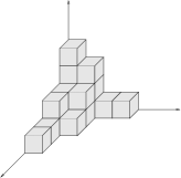
is the MacMahon function which enumerates plane partitions (three-dimensional Young diagrams) $\pi$ with $n=|\pi|$ boxes (see Fig. 1).

Figure 1: A three-dimensional Young diagram (plane partition) $\pi$. The corners of the upper boxes are located at lattice points $(i,j,\pi_{i,j})=(n_{1},n_{2},n_{3})\in\mathbb{Z}_{\geq 0}^{3}$ with $\pi_{i,j}\geq\pi_{i+1,j}$ and $\pi_{i,j}\geq\pi_{i,j+1}$. The total number boxes of $\pi$ is $|\pi|=\sum_{i,j}\,\pi_{i,j}$.

We use the convention $\chi(X)=1$ when $X={\mathbb{C}}^{3}$, so that

$${\cal Z}_{\rm BPS}^{{\mathbb{C}}^{3}}(q)=M(-q)\ .$$ (2.15)

2.2 Topological string theory

The Donaldson-Thomas partition function (2.7) is widely believed (and in some cases rigorously proven) to be equivalent via dualities to the partition function of the A-model topological string theory on the same threefold $X$. The topological A-model can be defined as a topological twist of an ${\cal N}=(2,2)$ superconformal sigma-model coupled to gravity. After localization onto classical (BRST) minima, the result is a theory of holomorphic maps

$$\phi\,:\,\Sigma_{g}\ \longrightarrow\ X$$ (2.16)

from a string worldsheet, which is a smooth projective curve $\Sigma_{g}$ of arithmetic genus $g\geq 0$, into the Calabi-Yau threefold $X$. This map describes a worldsheet instanton wrapping a curve in the homology class $\beta=\phi_{*}[\Sigma_{g}]\in H_{2}(X,{\mathbb{Z}})$. The string theory path integral of the topological A-model localizes onto a sum of integrals over the moduli spaces of these maps. Each (compactified) moduli space $\overline{{\mathscr{M}}}_{g,\beta}(X)$ parametrizes stable maps of genus $g$ wrapping a cycle $\beta$. The “number” of worldsheet instantons in each topological sector is computed via the “volume” of this moduli space as

$${\tt GW}_{g,\beta}(X)=\int_{[\,\overline{{\mathscr{M}}}_{g,\beta}(X)\,]^{\rm vir}}\ 1\ .$$ (2.17)

This formula defines the $\mathbb{Q}$-valued Gromov-Witten invariants of $X$. The integration is properly defined using a symmetric perfect obstruction theory in virtual dimension zero, which yields a virtual fundamental cycle $[\,\overline{{\mathscr{M}}}_{g,\beta}(X)\,]^{\rm vir}$ in the degree zero Chow group of subvarieties. The topological string amplitude has a genus expansion

$$F_{\rm top}^{X}(\lambda,Q)=\sum_{g=0}^{\infty}\,F^{X}_{g}(Q)\ \lambda^{2g-2}\qquad\mbox{with}\quad F^{X}_{g}(Q)=\sum_{\beta\in H_{2}(X,{\mathbb{Z}})}\ {\tt GW}_{g,\beta}(X)\ Q^{\beta}\ ,$$ (2.18)

where $\lambda=g_{s}$ is the string coupling, and the topological string partition function is

$$Z_{\rm top}^{X}(\lambda,Q)={\,\rm e}\,^{F_{\rm top}^{X}(\lambda,Q)}\ .$$ (2.19)

For toric threefolds $X$ the duality is based on the following observation. In the “classical” limit where the Kähler classes of $X$ are large, which is the limit $Q\to 0$ wherein the Calabi-Yau threefold is well approximated by gluing together ${\mathbb{C}}^{3}$ patches, the individual genus $g\geq 2$ amplitudes reduce to

$${\tt GW}_{g,0}(X)=\lim_{Q\to 0}\,F_{g}^{X}(Q)=\frac{\chi(X)}{2}\,\int_{\overline{{\mathscr{M}}}_{g}}\,c_{g-1}\left({\mathscr{H}}_{g}\right)^{\wedge 3}\ .$$ (2.20)

The topological string amplitude can thus be compactly expressed as an integral over Chern classes of the Hodge bundle ${\mathscr{H}}_{g}$ over the Deligne-Mumford moduli space $\overline{{\mathscr{M}}}_{g}$ of Riemann surfaces, whose fibre at a point $\Sigma_{g}$ is the complex vector space of holomorphic sections $H^{0}(\Sigma_{g},K_{\Sigma_{g}})$ of the canonical line bundle $K_{\Sigma_{g}}\to\Sigma_{g}$. This contribution comes from the constant maps: As the Kähler classes tend to infinity, every instanton contribution is suppressed and the path integral is well approximated by a sum over constant maps $\phi$ which take all of $\Sigma_{g}$ to a fixed point in $X$, with $\beta=0$. There are additional terms in genera $g=0,1$ which are divergent in this limit. The integrals in (2.20) were explicitly computed by Faber-Pandharipande [38] as

$$\int_{\overline{{\mathscr{M}}}_{g}}\,c_{g-1}\left({\mathscr{H}}_{g}\right)^{\wedge 3}=\frac{(-1)^{g}\,|B_{2g}\,B_{2g-2}|}{2g\,(2g-2)\,(2g-2)!}$$ (2.21)

with $B_{2g}$ the Bernoulli numbers for $g\geq 2$, and consequently [50]

$$\lim_{Q\to 0}\,Z_{\rm top}^{X}(\lambda,Q)=M(q)^{\chi(X)/2}$$ (2.22)

where $q=-{\,\rm e}\,^{{\,{\rm i}\,}\lambda}$ and $M(q)$ is the MacMahon function (2.14). Heuristically, if we send the Kähler classes to infinity, the topological string amplitude becomes a product of generating functions of three-dimensional Young diagrams, each factor associated with one of the copies of ${\mathbb{C}}^{3}$ needed to cover the Calabi-Yau manifold (in the sense of toric geometry), the total number of which is $\chi(X)$.

2.3 Topological vertex formalism

The proposed gauge/string theory duality can be stated precisely as the remarkable fact that the Gromov-Witten and Donaldson-Thomas partition functions are actually the same in the sense that [69]

$$Z_{\rm top}^{\,X}(\lambda,Q)=M(q)^{-\chi(X)/2}\ {{\cal Z}}_{\rm BPS}^{\,X}(q=-{\,\rm e}\,^{{\,{\rm i}\,}\lambda},Q)\ .$$ (2.23)

We interpret this equality as saying that the topological string amplitude captures the degeneracies of the D6–D2–D0 BPS bound states on a local threefold $X$. The duality can be extended to include open strings and topological D-branes which wrap Lagrangian submanifolds of a Calabi-Yau variety $X$.

This equality can be proven for toric manifolds $X$, wherein the partition functions can be evaluated combinatorially by applying virtual equivariant localization techniques to the BPS indices (2.11) with respect to the induced action of the three-torus ${\mathbb{T}}^{3}$ on the Hilbert scheme [69]. Localization involving virtual fundamental classes constructs a model for the virtual tangent space at the fixed points of the torus action: One considers the infinitesimal deformations around the fixed point and then subtracts the obstructions to these deformations. In this way one can regard the virtual tangent space roughly as the difference between two cohomology groups, and the relevant localization theorem gives the virtual Bott localization formula.

In the present case we can choose an affine cover of $X$ whose local charts $U_{\alpha}\cong\mathbb{C}^{3}$ are centred at the fixed points of the toric action. The integral (2.11) receives only two types of contributions, from the torus fixed points and the torus fixed lines in $X$, which correspond respectively to the vertices and edges of the toric diagram $\Delta$ of $X$. A torus fixed point $\pi_{\alpha}$ on $U_{\alpha}$ is represented by a monomial ideal

$$I_{\alpha}={\cal I}\big{|}_{U_{\alpha}}\ \subset\ {\mathbb{C}}[z_{1},z_{2},z_{3}]$$ (2.24)

which can be concretely represented by a three-dimensional Young diagram

$$\pi_{\alpha}=\big{\{}(m_{1},m_{2},m_{3})\in{\mathbb{Z}}^{3}_{\geq 0}\ \big{|}\ z_{1}^{m_{1}}\,z_{2}^{m_{2}}\,z_{3}^{m_{3}}\notin I_{\alpha}\big{\}}\ .$$ (2.25)

The second type of contribution comes from overlaps of two open charts $U_{\alpha}$ and $U_{\beta}$ which are glued along the line corresponding to $z_{1}$ to give

$$I_{\alpha\beta}={\cal I}\big{|}_{U_{\alpha}\cap U_{\beta}}\ \subset\ {\mathbb{C}}[z_{1}^{\pm\,1},z_{2},z_{3}]$$ (2.26)

and are represented by two-dimensional Young diagrams

$$\lambda_{\alpha\beta}=\big{\{}(m_{1},m_{2},m_{3})\ \big{|}\ z_{2}^{m_{2}}\,z_{3}^{m_{3}}\notin I_{\alpha\beta}\big{\}}\ .$$ (2.27)

A calculation in Čech cohomology then determines the contributions to the Euler characteristic $n=\chi({\cal I})$ [69].

The combinatorial evaluation of the partition function (2.7) thus boils down to decorating the trivalent planar toric graph $\Delta$ of $X$ with a three-dimensional Young diagram $\pi_{v}$ at each vertex $v$ and a two-dimensional Young diagram $\lambda_{e}$ at each edge $e$ representing the asymptotics of the infinite plane partition $\pi_{v}$. Symbolically, the partition function is then of the form

$${\cal Z}_{\rm BPS}^{X}(q,Q)=\sum_{\stackrel{{\scriptstyle\scriptstyle{\rm Young\ diagrams}}}{{\scriptstyle\lambda_{e}}}}\ \prod_{{\rm edges}\ e}\,Q_{e}^{|\lambda_{e}|}~{}\prod_{\stackrel{{\scriptstyle\scriptstyle{\rm vertices}}}{{\scriptstyle v=(e_{1},e_{2},e_{3})}}}\,M_{\lambda_{e_{1}},\lambda_{e_{2}},\lambda_{e_{3}}}(-q)$$ (2.28)

where

$$M_{\lambda,\mu,\nu}(q)=\sum_{\pi\,:\,\partial\pi=(\lambda,\mu,\nu)}\,q^{|\pi|}$$ (2.29)

is the generating function for plane partitions $\pi$ asymptotic to $(\lambda,\mu,\nu)$ with $M_{\emptyset,\emptyset,\emptyset}(q)=M(q)$; we set $\lambda_{e}=\emptyset$ on all external legs $e$ of the graph $\Delta$. The regularised box count $|\pi|$ of an infinite plane partition $\pi$ with boundary is computed using the degrees $(m_{e,1},m_{e,2})$ specifying the normal bundle ${\cal O}_{{\mathbb{P}}^{1}}(m_{e,1})\oplus{\cal O}_{{\mathbb{P}}^{1}}(m_{e,2})$ over the rational curve in $X$ corresponding to the given edge $e$ with the contribution

$$q^{\sum_{(i,j)\in\lambda_{e}}\,\left(m_{e,1}\,(i-1)+m_{e,2}\,(j-1)+1\right)+m_{e,1}\,|\lambda_{e}|}\ .$$ (2.30)

This gives the gluing rules for assembling three-dimensional and two-dimensional Young diagrams together; the “framing factors” (2.30) ensure that the gluing procedure doesn’t overcount or omit boxes when two plane partitions are glued together along an edge $e$. The localization integrals only contribute signs. It is shown in [89, 69] that (2.29) coincides (up to normalisation) with the topological vertex [4] in the melting crystal framework. Formally, the partition function (2.28) defines the statistical mechanics of a “Calabi-Yau crystal” and reproduces the topological string partition function within the formalism of the topological vertex. In this setting the boxes of the Young diagrams correspond to sections of the structure sheaves ${\cal O}_{Y}$ of the associated closed subschemes $Y\subset X$. A more general mathematical treatment of this algorithm, including classes of non-toric local Calabi-Yau threefolds involving non-planar graphs, can be found in [66].

In the following we will interpret the series (2.28) as a sum over generalized instantons in an auxilliary topological gauge theory on the D6-brane. They are states corresponding to ideal sheaves which can be thought of as singular gauge fields. In this setting the large radius BPS index (2.6) is regarded as the Witten index of the field theory on the D-branes, and hence the BPS partition function should be equivalent to the instanton partition function on the D-branes in this limit.

2.4 Conifold geometry

Let us work through an explicit example. The conifold singularity in six dimensions can be described as the locus $z_{1}\,z_{2}-z_{3}\,z_{4}=0$ in $\mathbb{C}^{4}$; the singularity at the origin can be removed by deforming the conifold to the locus $z_{1}\,z_{2}-z_{3}\,z_{4}=t$ with the deformation parameter $t$ thought of as the area of a projective line $\mathbb{P}^{1}$ replacing the origin. The crepant resolution of the conifold singularity is called the resolved conifold and it is described geometrically as the total space of a rank two holomorphic vector bundle ${\cal O}_{\mathbb{P}^{1}}(-1)\oplus{\cal O}_{\mathbb{P}^{1}}(-1)\to\mathbb{P}^{1}$. The toric diagram $\Delta$ consists of a single edge, representing the base $\mathbb{P}^{1}$, joining two trivalent vertices, representing the two $\mathbb{C}^{3}$ patches required to cover the resolved conifold.

The large radius partition function (2.28) reads

$${\cal Z}_{\rm BPS}^{\rm conifold}(q,Q) = \sum_{\lambda}\,M_{\emptyset,\emptyset,\lambda}(-q)\,M_{\emptyset,\emptyset,\lambda}(-q)\,Q^{|\lambda|}$$ (2.31)

$$= \sum_{\pi_{1},\pi_{2},\lambda}\,(-q)^{|\pi_{1}|+|\pi_{2}|+\sum_{(i,j)\in\lambda}\,(i+j+1)}\,Q^{|\lambda|}\ =\ M(-q)^{2}\,M(Q,-q)^{-1}\ ,$$

where the generating function

$$M(Q,q)=\prod_{n=1}^{\infty}\,\big{(}1-Q\,q^{n}\big{)}^{-n}$$ (2.32)

counts weighted plane partitions with $M(1,q)=M(q)$. In the “classical” limit $Q\to 0$ this reduces to $\big{(}{\cal Z}_{\rm BPS}^{\mathbb{C}^{3}}(q)\big{)}^{2}$, while the “undeformed” limit $Q\to 1$ gives ${\cal Z}_{\rm BPS}^{\mathbb{C}^{3}}(q)$, as expected.

In the setting of topological string theory, the constant map contributions ${\tt GW}_{g,0}({\rm conifold})$ for $g\geq 2$ are given by (2.21), while the two-homology of the resolved conifold is generated by its base ${\mathbb{P}}^{1}$ and the Gromov-Witten invariants which count worldsheet instantons are given by [38]

$${\tt GW}_{g,w}({\rm conifold})=-w^{2g-3}\,\frac{|B_{2g}|}{2g\,(2g-2)!}$$ (2.33)

for $g\geq 2$ and curve class $\beta=w\,[{\mathbb{P}}^{1}]$ with $w\in\mathbb{Z}$. The topological string amplitude is given by

$$F_{\rm top}^{\rm conifold}(\lambda,Q) = F^{\rm conifold}_{0}(Q)+F^{\rm conifold}_{1}(Q)$$

$$+\,\sum_{g=2}^{\infty}\,\lambda^{2g-2}\,\Big{(}\,\frac{(-1)^{g}\,|B_{2g}\,B_{2g-2}|}{2g\,(2g-2)\,(2g-2)!}-\frac{|B_{2g}|}{2g\,(2g-2)!}\,{\rm Li}_{3-2g}(Q)\,\Big{)}\ ,$$

where the genus zero contribution contains the intersection numbers and the instanton factor ${\rm Li}_{3}(Q)=\sum_{w\geq 1}\,\frac{Q^{w}}{w^{3}}$, the genus one part is given by the second Chern class of the tangent bundle of the conifold, and the polylogarithm function ${\rm Li}_{3-2g}(Q)=\sum_{w\geq 1}\,\frac{Q^{w}}{w^{3-2g}}$ sums the contributions from genus $g\geq 2$ worldsheet instantons. The gauge/string duality (2.23) (with $\chi(X)=2$) now follows from the exponential representation

$$M(Q,q)=\exp\Big{(}-\sum_{n=1}^{\infty}\,\frac{Q^{n}\,q^{n}}{n\,\big{(}1-q^{n}\big{)}^{2}}\,\Big{)}$$ (2.35)

of the generalized MacMahon function (2.32).

3 Counting modules over 3-Calabi-Yau algebras

3.1 Quiver gauge theories

So far we have been discussing ordinary Donaldson-Thomas invariants, which are a particular case of a generalized set of invariants defined over the whole Calabi-Yau moduli space that take into account the chamber structure and wall-crossing phenomena. We will now describe a different chamber, called the noncommutative crepant resolution chamber, wherein the geometry is described via the path algebra of a quiver, upon imposing a set of relations which can be derived from a superpotential. Physically this is the relevant situation that one encounters when a D3-brane is used as a probe of a singular Calabi-Yau threefold in a Type IIB compactification. The local geometry is reflected in the low-energy effective field theory which has the form of a quiver gauge theory, i.e. a field theory whose gauge and matter field content can be summarized in a representation of a quiver. This supersymmetric gauge theory is characterized by a superpotential which yields a set of relations as F-term constraints. The path algebra associated to the quiver is constrained by these relations; it encodes the geometry of the Calabi-Yau singularity and can be used to set up an interesting enumerative problem, where the roles of coherent sheaves are played by finitely-generated modules over this algebra in the standard dictionary of noncommutative algebraic geometry. Physically this corresponds to counting BPS states in the low-energy effective field theory; mathematically it goes under the name of noncommutative Donaldson-Thomas theory [95, 73].

Recall that a quiver $\sf Q$ is a directed graph specified by a set of vertices $v\in{\mathsf{Q}}_{0}$ and a set of arrows $\big{(}v\xrightarrow{\ a\ }w\big{)}\in{\mathsf{Q}}_{1}$ connecting vertices $v,w\in{\mathsf{Q}}_{0}$. Often a quiver comes with a set ${\mathsf{R}}$ of relations among its arrows. A path in the quiver is a set of arrows which compose; the relations ${\mathsf{R}}$ are realized as formal $\mathbb{C}$-linear combinations of paths. The paths modulo the ideal generated by the relations form an associative $\mathbb{C}$-algebra called the path algebra ${\mathsf{A}}={\mathbb{C}}\sf Q/\langle{\mathsf{R}}\rangle$, with product defined by concatenation of paths where possible and zero otherwise.

There is a particular class of quivers which come equipped with a superpotential ${\mathsf{W}}:{\mathsf{Q}}_{1}\to\mathbb{C}{\mathsf{Q}}$. In this case the mathematical definition of relations descends directly from the physical one: The relations of the quiver are the F-term equations derived from the superpotential, which is the ideal of relations generated by

$${\mathsf{R}}=\langle\partial_{a}{\mathsf{W}}\ |\ a\in{\mathsf{Q}}_{1}\rangle\ .$$ (3.1)

Here we regard $\sf{W}$ as a sum of cyclic monomials (since the gauge theory superpotential comes with a trace); the differentiation with respect to the arrow $a$ is then formally taken by cyclically permuting the elements of a monomial until $a$ is in the first position and then deleting it.

A (linear) representation of a quiver with relations $({\mathsf{Q}},{\mathsf{R}})$ is a collection of complex vector spaces $V_{v}$ for each vertex $v\in{\mathsf{Q}}_{0}$ together with a collection of linear transformations $B_{a}:V_{v}\to V_{w}$ for each arrow $\big{(}v\xrightarrow{\ a\ }w\big{)}\in{\mathsf{Q}}_{1}$ which respect the ideal of relations ${\mathsf{R}}$. The representations of a quiver with relations $(\sf Q,R)$ form a category ${{\mathfrak{R}}ep}(\sf Q,R)$ which is equivalent to the category ${\mathfrak{M}}od({\mathsf{A}})$ of finitely-generated left ${\mathsf{A}}$-modules. In quiver gauge theories one looks in general for representations of $({\mathsf{Q}},{\mathsf{R}})$ in the category of complex vector bundles (or better coherent sheaves), but in many cases the gauge theory is equivalently described by a matrix quantum mechanics for which it suffices to study the module category ${{\mathfrak{R}}ep}(\sf Q,R)$. We will be mostly interested in isomorphism classes of quiver representations which are orbits under the action of the gauge group $\prod_{v\in{\mathsf{Q}}_{0}}\,GL(V_{v},\mathbb{C})$; they can be characterised using geometric invariant theory. Equivalently, there is a more algebraic notion of stability of quiver representations introduced by King, which is closely related to the notion of stability for BPS states given by D-term constraints in supersymmetric gauge theories.

To each vertex $v$ we can associate a one-dimensional simple module ${\mathsf{D}}_{v}$ with $V_{v}={\mathbb{C}}$ and all other $V_{w}=0$; in string theory these modules correspond to fractional branes. Furthermore, if ${\mathsf{e}}_{v}$ is the trivial path at $v$ of length zero, then ${\mathsf{P}}_{v}:={\mathsf{e}}_{v}{\mathsf{A}}$ is the subspace of the path algebra generated by all paths that begin at vertex $v$; they are projective objects in the category ${{\mathfrak{R}}ep}(\sf Q,R)$ which can be used to construct projective resolutions of the simple modules through

(3.2)

where

$${d}^{p}_{w,v}=\dim\mathrm{Ext}^{p}_{\sf{A}}\left({\mathsf{D}}_{v},{\mathsf{D}}_{w}\right)\ .$$ (3.3)

Note that $d^{0}_{w,v}=\delta_{w,v}$ since ${\mathsf{D}}_{v}$ are simple objects; furthermore $d^{1}_{w,v}$ gives the number of arrows in ${\mathsf{Q}}_{1}$ from vertex $w$ to vertex $v$ and $d^{2}_{w,v}$ is the number of relations, while $d^{3}_{w,v}$ is the number of relations among the relations, and so on.

3.2 Noncommutative Donaldson-Thomas theory

When a D-brane probes a singular Calabi-Yau threefold, its low-energy effective field theory is typically encoded in a quiver diagram. From the geometry of the moduli space of the effective field theory one can reconstruct the Calabi-Yau singularity; it often happens that the singularity is resolved by quantum effects. We can abstract these facts into a mathematical statement: For Calabi-Yau singularities it is possible to find a certain noncommutative algebra ${\mathsf{A}}$ whose centre is the coordinate ring of the singularity and whose moduli spaces of representations are resolutions of the singularity. We call ${\mathsf{A}}$ the noncommutative crepant resolution of the singularity; the algebra ${\mathsf{A}}$ is finitely generated as a module over its centre and has the structure of a 3-Calabi-Yau algebra, see e.g. [48]. In the cases we are interested in, ${\mathsf{A}}$ is the path algebra of a quiver with relations.

On this noncommutative crepant resolution one can define Donaldson-Thomas invariants. The starting point is the low-energy effective field theory of a D2–D0 system on a toric Calabi-Yau threefold $X$. This system of branes has a “leg” outside $X$ in flat space ${\mathbb{R}}^{4}$; the effective field theory is the dimensional reduction to one dimension of four-dimensional ${\cal N}=1$ supersymmetric Yang-Mills theory. The end result is a supersymmetric quiver quantum mechanics with superpotential. Several techniques are available for determining this data. For example, Aspinwall-Katz have derived a fairly general formalism to compute the superpotential in [7]. Alternatively, the technology of brane tilings gives an efficient algorithm which has also a neat physical picture in terms of dualities [40, 42]; see [59, 104] for reviews. A more geometric perspective considers the toric geometry directly; then the quiver is derived through the endomorphisms of a tilting object, which guarantees that the derived category of representations of the quiver contains all geometric information encoded in the derived category of coherent sheaves on $X$. In the following we will assume that the relevant quiver ${\mathsf{Q}}$ and its superpotential $\sf W$ are known.

The path algebra ${\mathsf{A}}$ of this quiver with relations encoded in the superpotential is a noncommutative crepant resolution of the Calabi-Yau threefold $X$. However, the quiver so far represents only the effective field theory of the D2–D0 system. To incorporate the D6-brane we add an extra vertex $\{\bullet\}$ together with an additional arrow $a_{\bullet}$ from the new vertex to a reference vertex $v_{0}$ of ${\mathsf{Q}}$; this operation is a framing of the quiver and it ensures that the moduli space of representations has nice properties. We will denote the new quiver by $\hat{\mathsf{Q}}$; its vertex and arrow sets are given by

$$\hat{\mathsf{Q}}_{0}={\mathsf{Q}}_{0}\cup\{\bullet\}\qquad\mbox{and}\qquad\hat{\mathsf{Q}}_{1}={\mathsf{Q}}_{1}\cup\big{\{}\bullet\xrightarrow{\ a_{\bullet}\ }v_{0}\big{\}}\ .$$ (3.4)

This new quiver has its own path algebra $\hat{\mathsf{A}}$. Representations are now constructed by specifying an $n_{v}$-dimensional vector space $V_{v}$ on each node $v\in{\mathsf{Q}}_{0}$, while the framing node $\bullet$ always carries a one-dimensional vector space $\mathbb{C}$. Then the moduli space of stable representations ${\mathscr{M}}_{{\bm{n}}}(\hat{\mathsf{Q}},v_{0})$ characterized by the dimension vector ${{\bm{n}}}=(n_{v})_{v\in{\mathsf{Q}}_{0}}$ is compact and well behaved [73]; an appropriate symmetric perfect obstruction theory is developed in [95, 73], which gives a sensible notion of integration. The index of BPS D6–D2–D0 states is then the noncommutative Donaldson-Thomas invariant which is given by the weighted Euler characteristic of this moduli space as

$$\Omega_{{\mathsf{A}},v_{0}}({\bm{n}})={\tt DT}_{{\bm{n}},{v_{0}}}({\mathsf{A}}):=\chi\big{(}{\mathscr{M}}_{{\bm{n}}}(\hat{\mathsf{Q}},v_{0})\,,\,\nu_{\mathsf{A}}\big{)}\ ,$$ (3.5)

which again counts the “virtual” number of points. We can therefore define a partition function for the noncommutative Donaldson-Thomas invariants obtained from the path algebra ${\mathsf{A}}$ as

$${\cal Z}_{\rm BPS}^{{\mathsf{A}}}(p,v_{0})=\sum_{n_{v}\in{\mathbb{Z}}}\,\Omega_{{\mathsf{A}},v_{0}}({\bm{n}})\ \prod_{v\in{\mathsf{Q}}_{0}}\,p_{v}^{n_{v}}\ .$$ (3.6)

To set up an enumerative problem associated with the quiver, we begin from the state containing a single D6-brane and describe it as the space of paths on the quiver starting at the reference node $v_{0}$, modulo the F-term relations. We assign a different kind of box to each node of the quiver diagram by using different colours. This constructs a sort of “pyramid partition”, starting from the tip. In this enumerative problem only the nodes of $\sf Q$ enter: The extra framing node $\{\bullet\}$ plays only a passive role, in a certain sense fixing a “boundary condition” since it corresponds to the D6-brane which extends to infinity. The combinatorial construction is rendered more involved by the fact that at each step one has to impose the relations derived from the superpotential. The best way to rephrase the quiver relations into a practical rule is by the use of brane tilings and related techniques, see [73, 90]. The end result is that there is a direct correspondence between modules over the path algebra and the coloured pyramid partitions which are built.

The enumerative problem of noncommutative Donaldson-Thomas invariants is obtained by a combinatorial algorithm derived via virtual localization on the quiver representation moduli space with respect to a natural global action of a torus ${\mathbb{T}}$ which rescales the arrows and preserves the superpotential; the fixed points define ideals of the path algebra ${\mathsf{A}}$. Behrend-Fantechi prove in [12] that for a symmetric perfect obstruction theory like the ones constructed in [95, 73], which are compatible with the torus action, the contribution of an isolated ${\mathbb{T}}$-fixed point to the Euler characteristic (3.5) is given by a sign determined by the parity of the dimension of the tangent space at the fixed point. In particular, if all torus fixed points $\pi$ are isolated then we obtain [12, Thm. 3.4]

$${\tt DT}_{{\bm{n}},{v_{0}}}({\mathsf{A}})=\sum_{\pi\in{\mathscr{M}}_{{\bm{n}}}(\hat{\mathsf{Q}},v_{0})^{\mathbb{T}}}\,(-1)^{\dim T_{\pi}{\mathscr{M}}_{{\bm{n}}}(\hat{\mathsf{Q}},v_{0})}\ .$$ (3.7)

However, in constructing the low-energy effective field theory one loses track of the precise relation between box colours and D-brane charges. This change of variables can be explicitly determined in some simple examples, but no closed general formula has been found so far. This means that the BPS states thus enumerated have charges that can be non-trivial functions of the original D0 and D2 brane charges; in the noncommutative crepant resolution chamber the coloured partitions are the relevant dynamical variables and should be more properly thought of as “fractional branes” pinned to the singularity.

3.3 Conifold geometry

Let us look at the noncommutative crepant resolution of the conifold singularity discussed in §2.4. In this case the quiver ${\mathsf{Q}}$ is the Klebanov-Witten quiver [62], which contains two vertices ${\mathsf{Q}}_{0}=\{0,1\}$ and four arrows ${\mathsf{Q}}_{1}=\{a_{1},a_{2},b_{1},b_{2}\}$ with the quiver diagram

(3.8)

and superpotential

$${\sf W}=a_{1}\,b_{1}\,a_{2}\,b_{2}-a_{1}\,b_{2}\,a_{2}\,b_{1}\ .$$ (3.9)

The path algebra is given by

$${\sf A}={\mathbb{C}}[e_{0},e_{1}]\langle a_{1},a_{2},b_{1},b_{2}\rangle\,\big{/}\,\langle b_{1}\,a_{i}\,b_{2}-b_{2}\,a_{i}\,b_{1}\,,\,a_{1}\,b_{i}\,a_{2}-a_{2}\,b_{i}\,a_{1}\ |\ i=1,2\rangle\ .$$ (3.10)

The centre $Z({\mathsf{A}})$ of this algebra is generated by the elements

$$z_{1} = a_{1}\,b_{1}+b_{1}\,a_{1}\ ,$$

$$z_{2} = a_{2}\,b_{2}+b_{2}\,a_{2}\ ,$$

$$z_{3} = a_{1}\,b_{2}+b_{2}\,a_{1}\ ,$$

$$z_{4} = a_{2}\,b_{1}+b_{1}\,a_{2}\ ,$$ (3.11)

and hence

$${Z({\mathsf{A}})}={\mathbb{C}}[z_{1},z_{2},z_{3},z_{4}]\,\big{/}\,\left(z_{1}\,z_{2}-z_{3}\,z_{4}\right)$$ (3.12)

which corresponds precisely to the nodal singularity of the conifold. The path algebra ${\mathsf{A}}$ is thus a noncommutative crepant resolution of the conifold singularity.

To construct noncommutative Donaldson-Thomas invariants, we consider the framed conifold quiver

(3.13)

We want to study the moduli space of finite-dimensional representations of this quiver with relations that follow from the superpotential $\sf W$, or equivalently finite-dimensional left $\sf A$-modules. In particular, the moduli space of stable representations is now equivalent to the moduli space of cyclic modules. To construct this moduli space, one considers the representation space

$${\sf Rep}({\mathsf{Q}},v_{0})=\bigoplus_{(v\longrightarrow w)\in{{\mathsf{Q}}}_{1}}\,\mathrm{Hom}_{\mathbb{C}}(V_{v},V_{w})\ \oplus\ \mathrm{Hom}_{\mathbb{C}}(V_{0},{\mathbb{C}})\ ,$$ (3.14)

where we have introduced a vector space $V_{0}$, $V_{1}$ for each of the two nodes and the last summand corresponds to the framing arrow $a_{\bullet}$ to the reference node $v_{0}=0$. Now let ${\sf Rep}({\mathsf{Q}},v_{0};{\mathsf{W}})$ be the subspace obtained upon imposing the F-term equations derived from the superpotential $\sf W$ on ${\sf Rep}({\mathsf{Q}},v_{0})$. The moduli space is obtained by factoring the natural action of the gauge group by basis changes of the complex vector spaces $V_{0}$ and $V_{1}$ to get a smooth Artin stack

$${{\mathscr{M}}}_{n_{0},n_{1}}(\hat{\mathsf{Q}})=\big{[}{\sf Rep}({\mathsf{Q}},v_{0};{\mathsf{W}})\,\big{/}\,GL(n_{0},\mathbb{C})\times GL(n_{1},\mathbb{C})\big{]}\ ,$$ (3.15)

where we have dropped the reference vertex label for simplicity. After suitably defining the quotient, the resulting space has nice properties and carries a symmetric perfect obstruction theory [95].

Our task is now to compute the partition function for the noncommutative invariants

$${\cal Z}_{\rm BPS}^{\sf conifold}(p_{0},p_{1})=\sum_{n_{0},n_{1}\in{\mathbb{Z}}}\,{\tt DT}_{n_{0},n_{1}}({\mathsf{A}})\ p_{0}^{n_{0}}\,p_{1}^{n_{1}}\qquad\mbox{with}\quad{\tt DT}_{n_{0},n_{1}}({\mathsf{A}})=\chi\big{(}{{\mathscr{M}}}_{n_{0},n_{1}}(\hat{\mathsf{Q}})\,,\,\nu_{\mathsf{A}}\big{)}\ .$$ (3.16)

The invariants can be computed via equivariant localization with respect to a natural torus action which rescales the arrows diagonally; we keep only those transformations which leave the superpotential invariant. The relevant torus is thus

$${\mathbb{T}}={\mathbb{T}}_{{\mathsf{W}}}\,\big{/}\,S^{1}\ ,$$ (3.17)

where

$${\mathbb{T}}_{\mathsf{W}}=\big{\{}({\,\rm e}\,^{{\,{\rm i}\,}\epsilon_{1}},{\,\rm e}\,^{{\,{\rm i}\,}\epsilon_{2}},{\,\rm e}\,^{{\,{\rm i}\,}\epsilon_{3}},{\,\rm e}\,^{{\,{\rm i}\,}\epsilon_{4}})\ \big{|}\ \epsilon_{1}+\epsilon_{2}+\epsilon_{3}+\epsilon_{4}=0\big{\}}\ ,$$ (3.18)

while the subtorus

$$S^{1}\cong\big{\{}(\lambda,\lambda,\lambda^{-1},\lambda^{-1})\ \big{|}\ \lambda\in S^{1}\big{\}}$$ (3.19)

is dictated by the charge vector which characterizes the resolved conifold as a toric variety. To evaluate the invariants we therefore need to classify the fixed points of this toric action on the moduli space and compute the contributions of each fixed point. In [95] Szendrői proves that there is a bijective correspondence between the set of fixed points and the set $\mathcal{P}$ of plane partitions $\pi$ such that if a box is present in $\pi$ then so are the boxes immediately above it, which are of two different colours, say black and white. Elements $\pi\in{\cal P}$ are called pyramid partitions (see Fig. 2).

Figure 2: A pyramid partition $\pi\in\mathcal{P}$.

These combinatorial arrangements are examples of those we discussed in §3.2; the enumeration of BPS states proceeds from the framed conifold quiver via the combinatorial algorithm that we sketched there.

To assemble this data into the partition function (3.16), all that is left to do is compute the contribution of each fixed point $\pi\in\mathcal{P}$, for which [95] proves

$$(-1)^{\dim T_{\pi}{{\mathscr{M}}}_{n_{0},n_{1}}(\hat{\mathsf{Q}})}=(-1)^{|\pi_{1}|}$$ (3.20)

where $n_{1}=|\pi_{1}|$ is the number of black boxes in the pyramid partition $\pi$. If we similarly denote by $n_{0}=|\pi_{0}|$ the number of white boxes, then the generating function of noncommutative Donaldson-Thomas invariants assumes the form

$${\cal Z}_{\rm BPS}^{\sf conifold}(p_{0},p_{1})=\sum_{\pi\in\mathcal{P}}\,(-1)^{|\pi_{1}|}\ p_{0}^{|\pi_{0}|}\,p_{1}^{|\pi_{1}|}\ .$$ (3.21)

This partition function has a nice infinite product representation [105]: If we change variables to $q=p_{0}\,p_{1}$ and $Q=p_{1}$ then

$${\cal Z}_{\rm BPS}^{\sf conifold}(q,Q)=M(-q)^{2}\,M(Q,-q)\,M(Q^{-1},-q)\ .$$ (3.22)

It is interesting to compare the partition function (3.22) with the large radius generating function (2.31) of the ordinary Donaldson-Thomas invariants. Szendrői notes there is a product formula that expresses the noncommutative invariants in terms of the ordinary Donaldson-Thomas invariants of the two (commutative) crepant resolutions of the conifold singularity, which are mutually related by a flop transition where the two-cycle shrinks to zero size. If we label them by $\pm$, then

$${\cal Z}_{\rm BPS}^{{\rm conifold}^{-}}(q,Q)=M(-q)^{2}\,M(Q,-q)\qquad\mbox{and}\qquad{\cal Z}_{\rm BPS}^{{\rm conifold}^{+}}(q,Q)=M(-q)^{2}\,M(Q^{-1},-q)\ ,$$ (3.23)

where now the parameter $Q$ is interpreted as the large radius Kähler parameter ${\,\rm e}\,^{-t}$. Then one has the surprising equality

$${\cal Z}_{\rm BPS}^{\sf conifold}(q,Q)=M(-q)^{-2}\ {\cal Z}_{\rm BPS}^{{\rm conifold}^{-}}(q,Q)\,{\cal Z}_{\rm BPS}^{{\rm conifold}^{+}}(q,Q)\ .$$ (3.24)

This formula is interpreted as saying that the partition function of noncommutative Donaldson-Thomas invariants can be obtained from the topological string partition function from a number of wall crossings.

4 Counting curves in toric surfaces

4.1 BPS states and Hilbert schemes

In order to set up the gauge theory formulation of the curve counting problems on Calabi-Yau threefolds, we shall start in a setting wherein the gauge theory problem (instanton counting) has been more thoroughly investigated and is much better understood. In the next few sections we will study the relationship between curve counting and gauge theory on a general toric surface $M$, in particular with the enumeration of instantons in four dimensions. However, even in the simplest $U(1)$ cases, surprisingly little is understood rigorously in full generality; the best understood classes of toric surfaces are ALE spaces and Hirzebruch surfaces. One of our goals in the following will be an attempt to set up a rigorous framework that computes the gauge theory partition functions on generic Hirzebruch-Jung spaces. Geometrically, the respective problems correspond to counting subschemes of dimension zero and one with compact support in a surface $M$, and counting rank one torsion free sheaves ${\cal T}$ on $M$ which now have the factorized form

$${\cal T}={\cal L}\otimes{\cal I}$$ (4.1)

where ${\cal L}={\cal T}^{\vee\vee}$ is a line bundle and ${\cal I}$ is an ideal sheaf of points; compared to the six-dimensional case, the extra factor ${\cal L}$ is necessary to include one-dimensional subschemes which in this case occur as components in codimension one. From the gauge theory perspective, the main difference from Donaldson-Thomas theory is now the presence of a non-trivial first Chern class. This is essentially the reason why the two problems are different. As we have defined them, Donaldson-Thomas invariants count bound states of D6–D2–D0 branes. Adding D4-branes which wrap compact four-cycles yields sheaves with non-trivial first Chern class. In the following we will enumerate BPS D2–D0 bound states in D4-branes which wrap a toric surface $M$ inside a Calabi-Yau threefold $X$ without D6-branes.

The pertinent moduli space is again the Hilbert scheme ${\mathscr{M}}^{\rm BPS}_{n,\beta}(M)={\rm Hilb}_{n,\beta}(M)$ of compact curves $Y\subset M$ with

$$n=\chi({\cal O}_{Y})\qquad\mbox{and}\qquad\beta=[Y]\ \in\ H_{2}(M,\mathbb{Z})\ .$$ (4.2)

For any smooth projective surface $M$, the structure of this scheme simplifies tremendously, and it is a smooth manifold. In this case a codimension one subscheme of $M$ factorizes into divisors, and sums of free and embedded points. This implies that the Hilbert scheme factorizes into divisorial and punctual parts as

$${\mathscr{M}}^{\rm BPS}_{n,\beta}(M)\cong{\rm Div}_{\beta}(M)\times{\rm Hilb}_{n-n_{\beta}}(M)\ .$$ (4.3)

The intersection number

$$n_{\beta}=-\mbox{$\frac{1}{2}$}\,\langle\beta,\beta+K_{M}\rangle_{\Gamma}$$ (4.4)

is the contribution of the divisorial part $D$ of a subscheme $Y\in{\mathscr{M}}^{\rm BPS}_{n,\beta}(M)$ with $[D]=\beta$ to the holomorphic Euler characteristic $n=\chi({\cal O}_{Y})$, with $K_{M}=-c_{1}(M)$ the canonical class of $M$, and ${\rm Div}_{\beta}(M):={\rm Hilb}_{n_{\beta},\beta}(M)$ is the projective moduli space of divisors in $M$. The remainder due to free and embedded points of $Y$ is contained in the Hilbert scheme ${\rm Hilb}_{m}(M)$ of $m=n-n_{\beta}$ points on $M$, which in this case is non-singular of dimension $2m$.

Thus in this case the moduli space ${\mathscr{M}}^{\rm BPS}_{n,\beta}(M)$ is smooth, and we can define generating functions using ordinary fundamental classes, without recourse to virtual cycles as before. In particular, we define the partition function for D4–D2–D0 BPS bound states on $M$ as

$${\cal Z}_{\rm BPS}^{M}(q,Q)=\sum_{\beta\in H_{2}(M,{\mathbb{Z}})}\,Q^{\beta}\ Z_{\beta}^{M}(q)\qquad\mbox{with}\quad Z_{\beta}^{M}(q)=\sum_{n\in{\mathbb{Z}}}\,q^{n}\ \Omega_{M}(n,\beta)\ ,$$ (4.5)

where now the index of BPS states is given by the topological Euler characteristic

$$\Omega_{M}(n,\beta):=\chi\big{(}{\mathscr{M}}^{\rm BPS}_{n,\beta}(M)\big{)}=\int_{{\mathscr{M}}^{\rm BPS}_{n,\beta}(M)}\,{\rm eul}\big{(}T{\mathscr{M}}^{\rm BPS}_{n,\beta}(M)\big{)}$$ (4.6)

with ${\rm eul}\big{(}T{\mathscr{M}}^{\rm BPS}_{n,\beta}(M)\big{)}$ the Euler class of the stable tangent bundle on the smooth moduli space ${\mathscr{M}}^{\rm BPS}_{n,\beta}(M)$. The analog of the formula (2.13) for the degree zero contributions are now encoded by Göttsche’s formula

$$Z_{0}^{M}(q)=\sum_{n=0}^{\infty}\,q^{n}\ \chi\big{(}{\rm Hilb}_{n}(M)\big{)}=\hat{\eta}(q)^{-\chi(M)}$$ (4.7)

for the generating function of the Euler characteristics of Hilbert schemes of points on surfaces, where $\hat{\eta}(q)$ is the Euler function whose inverse

$$\hat{\eta}(q)^{-1}=\prod_{n=1}^{\infty}\,\big{(}1-q^{n}\big{)}^{-1}=\sum_{\lambda}\,q^{|\lambda|}$$ (4.8)

enumerates two-dimensional Young diagrams (partitions) $\lambda=(\lambda_{1},\lambda_{2},\dots)$, $\lambda_{i}\geq\lambda_{i+1}$ with $n=|\lambda|=\sum_{i}\,\lambda_{i}$ boxes.

4.2 Vertex formalism

The Euler characteristics (4.6) can be evaluated by applying the localization theorem in equivariant Chow theory due to Edidin-Graham [37]. In our case the localization formula is simplified by the fact that the fixed point locus of the toric action on the moduli space ${\mathscr{M}}^{\rm BPS}_{n,\beta}(M)$, induced by the action of the two-torus ${\mathbb{T}}^{2}$ on $M$, consists of isolated points and the integrand is the Euler class of the tangent bundle, which cancels against the tangent weights coming from the localization formula. The collection of ${\mathbb{T}}^{2}$-invariant ideal sheaves specifying the one-dimensional subschemes $Y$ is in bijective correspondence with the set of all (possibly infinite) Young tableaux; in contrast to the case of plane partitions, there is a simple factorization of infinite two-dimensional Young diagrams into a finite part plus their asymptotic limits which we denote symbolically by

$$\{\mbox{infinite Young diagrams}\}~{}\cong~{}\mathbb{Z}_{\geq 0}^{2}\ \times\ \{\mbox{finite Young diagrams}\}\ .$$ (4.9)

This factorization is depicted in Fig. 3 and it corresponds to the decomposition (4.3) of a subscheme $Y$ into a reduced and a zero-dimensional component.

Figure 3: Factorization of an infinite two-dimensional Young diagram into a finite Young diagram $\pi_{i,i+1}$ and its boundaries along the two coordinate axes which are specified by integers $\lambda_{i},\lambda_{i+1}\in\mathbb{Z}_{\geq 0}$. Here $i$ labels the one-cones of the toric fan of $M$, while $(i,i+1)$ labels the two bounding one-cones of each toric fixed point on $M$.

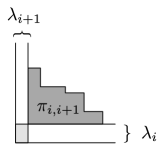
The contribution of the free and embedded points to the holomorphic Euler characteristic $n=\chi({\cal O}_{Y})$ is given by the total box count of the finite parts of Young diagrams, while for any compact toric invariant divisor $D$ with an expansion $D=\sum_{i}\,\lambda_{i}\,D_{i}$, $\lambda_{i}\in\mathbb{Z}_{\geq 0}$ in a basis of ${\mathbb{T}}^{2}$-invariant divisors $D_{i}$ with self-intersection numbers $\alpha_{i}=-\langle D_{i},D_{i}\rangle_{\Gamma}$, a computation in Čech cohomology shows [24]

$$\chi({\cal O}_{D})=-\mbox{$\frac{1}{2}$}\,\langle D,D+K_{M}\rangle_{\Gamma}=\sum_{i}\,\big{(}\mbox{$\frac{1}{2}$}\,\alpha_{i}\,\lambda_{i}\,(\lambda_{i}-1)+\lambda_{i}-\lambda_{i}\,\lambda_{i+1}\big{)}\ .$$ (4.10)

Using this data one can combinatorially evaluate the BPS partition function (4.5) via a vertex formalism for toric surfaces $M$ which is analogous to the topological vertex formalism for toric threefolds discussed in §2.3. The partition function is constructed on the bivalent planar toric graph $\Delta$ which is the dual web diagram of the toric fan of $M$. This formalism associates to each vertex $v=(e_{1},e_{2})$, where two edges $e_{1}$ and $e_{2}$ of $\Delta$ meet, a factor

$$V_{\lambda_{e_{1}},\lambda_{e_{2}}}(q)=\hat{\eta}(q)^{-1}~{}q^{-\lambda_{e_{1}}\,\lambda_{e_{2}}}\ ,$$ (4.11)

where the inverse Euler function $\hat{\eta}(q)^{-1}$ counts two-dimensional Young diagrams based at the vertex and the two non-negative integers $\lambda_{e_{1}},\lambda_{e_{2}}$ label the asymptotics of the partitions along the edges connecting two vertices with the product $\lambda_{e_{1}}\,\lambda_{e_{2}}$ the contribution to the regularized box count of an infinite Young diagram. Two vertices are glued together along an edge $e$ carrying the common label $\lambda_{e}$ by a “propagator”

$$G_{\lambda_{e}}(q,Q_{e})=q^{\frac{1}{2}\,\alpha_{e}\,\lambda_{e}\,(\lambda_{e}-1)+\lambda_{e}}\ Q_{e}^{\lambda_{e}}\ ,$$ (4.12)

where $\alpha_{e}$ is the self-intersection number of the rational curve represented by the edge $e$ and the parameter $Q_{e}$ weighs the homology class of the edge. Then the partition function has the symbolic form

$${\cal Z}_{\rm BPS}^{M}(q,Q)=\sum_{\lambda_{e}\in\mathbb{Z}_{\geq 0}}~{}\prod_{{\rm edges}\ e}\,G_{\lambda_{e}}(q,Q_{e})~{}\prod_{\stackrel{{\scriptstyle\scriptstyle{\rm vertices}}}{{\scriptstyle v=(e_{1},e_{2})}}}\,V_{\lambda_{e_{1}},\lambda_{e_{2}}}(q)\ ,$$ (4.13)

where we set $\lambda_{e}=0$ on all external legs $e$ of the graph $\Delta$. Since there is a factor $\hat{\eta}(q)^{-1}$ for each vertex, the partition function (4.13) carries an overall factor $\hat{\eta}(q)^{-\chi(M)}$ associated to the degree zero contributions as in Göttsche’s formula (4.7), where $\chi(M)$ is the topological Euler characteristic of $M$. It would be interesting to find a four-dimensional version of topological string theory which reproduces this counting, analogously to §2.

4.3 Hirzebruch-Jung surfaces

Our main examples of toric surfaces in this paper will fall into the general class of Hirzebruch-Jung spaces $M=M_{p,p^{\prime}}$, which are resolutions of $A_{p,p^{\prime}}$ singularities for a pair of coprime integers $p>p^{\prime}>0$; they represent the most general toric singularity in four dimensions. In this case we may regard $M$ as a four-cycle in the Calabi-Yau threefold $X=K_{M}$. Consider the quotient of ${\mathbb{C}}^{2}$ by the action of the cyclic group $G_{p,p^{\prime}}\cong\mathbb{Z}_{p}$ generated by

$$G_{p,p^{\prime}}=\mbox{$\frac{1}{p}$}\,\big{(}1\,,\,p^{\prime}\,\big{)}:=\left(\begin{matrix}\zeta&0\\ 0&\zeta^{p^{\prime}}\\ \end{matrix}\right)$$ (4.14)

where $\zeta={\,\rm e}\,^{2\pi{\,{\rm i}\,}/p}$. In the framework of toric geometry this singular space is described by the two-cone spanned by two lattice vectors ${\sf v}_{0}=(1,0)$ and ${\sf v}_{m+1}=(-p^{\prime},p)$ in $\mathbb{Z}^{2}$. The minimal resolution $\pi:M_{p,p^{\prime}}\rightarrow{\mathbb{C}}^{2}/G_{p,p^{\prime}}$ is the smooth connected moduli space $\mathrm{Hilb}_{G_{p,p^{\prime}}}({\mathbb{C}}^{2})$ consisting of $G_{p,p^{\prime}}$-clusters, i.e. $G_{p,p^{\prime}}$-invariant zero-dimensional subschemes $Z$ of ${\mathbb{C}}^{2}$ of length $|G_{p,p^{\prime}}|$ such that $H^{0}({\cal O}_{Z})$ is the regular representation of $G_{p,p^{\prime}}$. The toric diagram of $M_{p,p^{\prime}}=\mathrm{Hilb}_{G_{p,p^{\prime}}}({\mathbb{C}}^{2})$ is obtained by the subdivision with one-cones ${\sf v}_{1},\ldots,{\sf v}_{m}$ such that

$${\sf v}_{i-1}+{\sf v}_{i+1}=\alpha_{i}\,{\sf v}_{i}$$ (4.15)

for $i=1,\ldots,m$, where the integers $m$ and $\alpha_{i}\geq 2$ are determined by the continued fraction expansion

$$\frac{p}{p^{\prime}}=[\alpha_{1},\dots,\alpha_{m}]:=\alpha_{1}-\frac{1}{\alpha_{2}-\displaystyle{\frac{1}{\alpha_{3}-\displaystyle{\frac{1}{\ddots\,\displaystyle{\alpha_{m-1}-\frac{1}{\alpha_{m}}}}}}}}\ .$$ (4.16)

Geometrically the singularity is resolved by a chain of $m$ exceptional divisors $D_{i}\cong{\mathbb{P}}^{1}$ whose intersection matrix is

$$C=\big{(}\langle D_{i},D_{j}\rangle_{\Gamma}\big{)}=\begin{pmatrix}-\alpha_{1}&1&0&\cdots&0\\ 1&-\alpha_{2}&1&\cdots&0\\ 0&1&-\alpha_{3}&\cdots&0\\ \vdots&\vdots&\vdots&\ddots&\vdots\\ 0&0&0&\cdots&-\alpha_{m}\end{pmatrix}\ .$$ (4.17)

The exceptional curves $D_{i}$, $i=1,\dots,m$ generate the Mori cone in the rational Chow group $H_{2}^{c}(M_{p,p^{\prime}},\mathbb{Q})$ consisting of linear combinations of compact algebraic cycles with non-negative coefficients.

The vertex rules determine the BPS partition function (4.13) as

$${\cal Z}_{\rm BPS}^{M_{p,p^{\prime}}}(q,Q)=\frac{1}{\hat{\eta}(q)^{m+1}}\ \sum_{\lambda_{i}\in\mathbb{Z}_{\geq 0}}\,q^{-\frac{1}{2}\,\lambda\cdot C\lambda+\frac{1}{2}\,\lambda\cdot C\delta+\frac{1}{2}\,\lambda_{1}+\frac{1}{2}\,\lambda_{m}}\ Q^{\lambda}$$ (4.18)

where $\delta:=(1,\dots,1)$. In particular, the spaces $M_{p+1,p}$ are the Calabi-Yau ALE resolutions of $A_{p}$ singularities consisting of a chain of $m=p$ exceptional divisors $D_{i}$, for which $\alpha_{i}=2$ for $i=1,\ldots,p$, $K_{M_{p+1,p}}=0$, and (4.17) coincides with minus the Cartan matrix of the $A_{p}$ Dynkin diagram which represents the toric graph $\Delta$; the partition function in this case simplifies to

$${\cal Z}_{\rm BPS}^{A_{p}}(q,Q)=\frac{1}{\hat{\eta}(q)^{p+1}}\ \sum_{\lambda_{i}\in\mathbb{Z}_{\geq 0}}\,q^{-\frac{1}{2}\,\lambda\cdot C\lambda}\ Q^{\lambda}\ .$$ (4.19)

On the other hand, for $p^{\prime}=1$ there is only one exceptional divisor with self-intersection number $-\alpha_{1}=-p$ and the manifold $M_{p,1}$ can be regarded as the total space of a holomorphic line bundle ${\cal O}_{\mathbb{P}^{1}}(-p)$ of degree $p$ over the projective line $\mathbb{P}^{1}$; the geometry is the natural analog of the resolved conifold geometry from §2.4. This space has a toric projectivization to the $p$-th Hirzebruch surface $\mathbb{F}_{p}$ and the partition function is given by

$${\cal Z}_{\rm BPS}^{\mathbb{F}_{p}}(q,Q)=\frac{1}{\hat{\eta}(q)^{2}}\,\sum_{\lambda=0}^{\infty}\,q^{\frac{p}{2}\,\lambda^{2}}\ Q^{\lambda}\ .$$ (4.20)

5 Four-dimensional cohomological gauge theory

5.1 Vafa-Witten theory on toric surfaces

A natural candidate gauge theory dual to the curve counting theory of BPS states discussed in §4 is the topological gauge theory studied by Vafa-Witten [98], defined on four-dimensional toric manifolds. This is the low-energy effective field theory on D4-branes wrapping a holomorphic divisor $M$ in a Calabi-Yau threefold [13, 97]; the counting of instantons on D4-branes is then equivalent to the enumeration of BPS D2–D0 staes in the D4-branes, and hence we would expect the instanton partition function to be equivalent to the BPS partition function for D4–D2–D0 bound states. Under favourable circumstances, this gauge theory captures the holomorphic sector of ${\cal N}=4$ supersymmetric Yang-Mills theory in four dimensions and can be used to understand its modular properties under S-duality transformations (when viewed as a function of the elliptic modulus $q$). This is particularly interesting on non-compact toric manifolds, such as the $A_{p}$ series of ALE spaces considered by Kronheimer-Nakajima [64]. On these spaces, by using celebrated results of Nakajima [78], Vafa-Witten relate the partition function of the topological gauge theory with the characters of an affine Lie algebra, thereby completely characterizing it as a quasi-modular form. In subsequent sections we will extend these considerations to a relation between Donaldson-Thomas theory and topological Yang-Mills theory in six dimensions.

Here we consider the topologically twisted version of ${\cal N}=4$ supersymmetric Yang-Mills theory with gauge group $G$ as constructed in [98] on a smooth connected Kähler surface $(M,t)$; in the four-dimensional cases we will always set $B=0$. When certain conditions are met (the Vafa-Witten vanishing theorems) the corresponding partition function computes the Euler characteristic of the instanton moduli space. The space of fields ${\mathscr{W}}$ is given by

$${\mathscr{W}}={\mathscr{A}}({\cal P})\times\Omega^{0}\left(M,\mathrm{ad}\,{\cal P}\right)\times\Omega^{2,+}\left(M,\mathrm{ad}\,{\cal P}\right)$$ (5.1)

where ${\mathscr{A}}({\cal P})$ denotes the affine space of connections on a principal $G$-bundle ${\cal P}\rightarrow M$, $\mathrm{ad}\,{\cal P}$ is the adjoint bundle of ${\cal P}$, and the superscript $+$ denotes the self-dual part; the superpartners of the fields in (5.1) are sections of the tangent bundle over ${\mathscr{W}}$. For $(A,\phi,b^{+})\in{\mathscr{W}}$, the twisted gauge theory corresponds to the moduli problem associated with the field equations

$$\sigma := F_{A}^{+}+\mbox{$\frac{1}{4}$}\,t^{-1}\big{(}b^{+}\wedge b^{+}\big{)}+\mbox{$\frac{1}{2}$}\,\phi\wedge b^{+}\ =\ 0\ ,$$

$$\kappa := t^{-1}\big{(}\nabla_{A}b^{+}\big{)}+\nabla_{A}\phi\ =\ 0\ ,$$ (5.2)

where $F_{A}$ is the curvature of the gauge connection one-form $A$ and $\nabla_{A}$ the associated covariant derivative, and the adjoint section $\phi$ is called a Higgs field. Associated with these field equations are a pair of doublets which are sections of the bundle ${\mathscr{F}}=\Omega^{2,+}\left(M,\mathrm{ad}\,{\cal P}\right)\oplus\Omega^{1}\left(M,\mathrm{ad}\,{\cal P}\right)$.

The path integral of the topological gauge theory localizes onto the solutions of the field equations (5.2). The partition function can be interpreted geometrically as a Mathai-Quillen representative of the Thom class of the bundle $\mathscr{V}=\mathscr{W}\times_{\cal{G}({\cal P})}\mathscr{F}$, and its pullback via the sections $(\sigma,\kappa)$ of (5.2) gives the Euler class of $\mathscr{V}$; here $\mathcal{G}({\cal P})$ is the group of gauge transformations, which are automorphisms of the $G$-bundle ${\cal P}\to M$. Under favourable conditions, appropriate vanishing theorems hold which ensure that each solution of the system (5.2) has $\phi=b^{+}=0$ and corresponds to an instanton, i.e. an anti-self-dual connection; the space of gauge equivalence classes of solutions to the anti-self-duality equations $F_{A}^{+}=0$ is called the instanton moduli space $\mathscr{M}^{\rm inst}_{\cal P}(M)$. Then the path integral localizes onto $\mathscr{M}^{\rm inst}_{\cal P}(M)$ and reproduces a representative of the Euler class of the tangent bundle $T\mathscr{M}^{\rm inst}_{\cal P}(M)$. Therefore the partition function computes volumes of the form

$$\chi\big{(}\mathscr{M}^{\rm inst}_{\cal P}(M)\big{)}=\int_{\mathscr{M}^{\rm inst}_{\cal P}(M)}\,{\rm eul}\big{(}T\mathscr{M}^{\rm inst}_{\cal P}(M)\big{)}$$ (5.3)

which give the Euler character of the moduli space of $G$-instantons on $M$; it can be computed from the index of the Atiyah-Hitchin-Singer instanton deformation complex [65]

(5.4)

associated with the equations (5.2), where the first morphism is an infinitesimal gauge transformation while the second morphism corresponds to the linearization of the sections $(\sigma,\kappa)$. For unitary gauge bundles ${\cal E}\to M$ of rank $r$, the moduli space can be stratified into connected components ${\mathscr{M}}^{\rm inst}_{n,u;r}(M)$ with fixed instanton and monopole charges

$$n={\rm ch}_{2}({\cal E})\ \in\ H^{4}(M,\mathbb{Z})=\mathbb{Z}\qquad\mbox{and}\qquad u=c_{1}({\cal E})\ \in\ H^{2}(M,\mathbb{Z})\ .$$ (5.5)

Let us now look at the rank one case and embed the moduli space of $U(1)$ bundles with anti-self-dual connection into the space of (semi-stable) torsion free sheaves ${\cal T}$; this embedding provides a smooth Gieseker compactification of the instanton moduli space which can be naturally thought of as algebraic geometry data parametrizing the extension of the moduli space to include noncommutative instantons. We can organize the moduli space of isomorphism classes of these sheaves according to their Chern classes as ${\mathscr{M}}^{\rm inst}_{n,\beta}(M)$ with

$$n={\rm ch}_{2}({\cal T})\qquad\mbox{and}\qquad\beta=c_{1}({\cal T})\ \in\ H_{2}(M,{\mathbb{Z}})\ ,$$ (5.6)

where we use Poincaré-Chow duality for surfaces to regard divisors of $M$ both as curves and as degree two cohomology classes. Note that for non-compact spaces the second Chern characteristic class $n$ can be fractional. The factorization (4.1) implies an analogous factorization of the moduli space strata

$${\mathscr{M}}^{\rm inst}_{n,\beta}(M)\cong\mathrm{Pic}_{\beta}(M)\times{\rm Hilb}_{n-n_{\beta}}(M)\ ,$$ (5.7)

similarly to (4.3). The Picard lattice $\mathrm{Pic}_{\beta}(M)$ parametrizes isomorphism classes of holomorphic line bundles ${\cal L}={\cal O}_{M}(D)$ of divisors $D$ on $M$ with $[D]=\beta$ which contribute the intersection number (4.4) to the second Chern characteristic of a torsion free sheaf and which are called “fractional” instantons, while the Hilbert scheme of points ${\rm Hilb}_{m}(M)$ is the smooth manifold of dimension $2m$ which parametrizes ideal sheaves ${\cal I}_{Z}$ with instanton number $m$ (and $c_{1}({\cal I}_{Z})=0$) corresponding to “regular” instantons supported on a zero-dimensional subscheme $Z\subset M$ of length $m=n-n_{\beta}$. Using the Grothendieck-Riemann-Roch formula, the contribution of a primitive element of (5.7) to the instanton number $n$ is found to be [24]

$${\rm ch}_{2}\big{(}{\cal O}_{M}(D)\otimes{\cal I}_{Z}\big{)}=\mbox{$\frac{1}{2}$}\,\langle D,D\rangle_{\Gamma}-\chi({\cal O}_{Z})$$ (5.8)

with $\langle D,D\rangle_{\Gamma}=\int_{M}\,c_{1}({\cal O}_{M}(D))\wedge c_{1}({\cal O}_{M}(D))$.

The gauge theory partition function is given by

$$Z_{\rm gauge}^{M}(q,Q)=\sum_{n,\beta}\,q^{n}\ Q^{\beta}\ \int_{{\mathscr{M}}^{\rm inst}_{n,\beta}(M)}\,{\rm eul}\big{(}T{\mathscr{M}}^{\rm inst}_{n,\beta}(M)\big{)}\ .$$ (5.9)

By Göttsche’s formula (4.7), the regular instantons contribute to (5.9) with a factor $\hat{\eta}(q)^{-\chi(M)}$ which is identical to that of the BPS partition function (4.13). On the other hand, the discrete factor which comes from the sum over fractional instantons ${\cal L}\in{\rm Pic}_{\beta}(M)$ is different from that of (4.13); this series is a generalized theta-function which carries the relevant information about the partition function as a quasi-modular form. Hence the curve counting and instanton counting problems are related but not identical in four dimensions; we shall see later on that the duality is however exact in six dimensions.

For illustration, let us consider the class of Hirzebruch-Jung spaces from §4.3. In this case, using linear equivalence one can extend the complete set of torically invariant divisors, including the non-compact ones, to an integral generating set for the Picard group ${\rm Pic}(M_{p,p^{\prime}})\cong H^{2}(M_{p,p^{\prime}},\mathbb{Z})=\mathbb{Z}^{m}$ of line bundles given by [24]

$$e^{i}=\sum_{j=1}^{m}\,\big{(}C^{-1}\big{)}^{ij}\,D_{j}\qquad\mbox{for}\quad i=1,\dots,m\ ,$$ (5.10)

where the matrix $C_{ij}=\langle D_{i},D_{j}\rangle_{\Gamma}$ is the integer-valued intersection form (4.17) for the compact two-cycles of the resolution $M_{p,p^{\prime}}$ whose inverse can be found in e.g. [51, App. A]. These divisors satisfy

$$\big{\langle}D_{i}\,,\,e^{j}\,\big{\rangle}_{\Gamma}=\delta_{i}{}^{j}\ ,$$ (5.11)

and hence generate the Kähler cone which is the polyhedron in the rational Chow group $H^{2}(M_{p,p^{\prime}},\mathbb{Q})$ dual to the Mori cone with respect to the intersection pairing

$$\langle-,-\rangle_{\Gamma}\,:\,H_{2}^{c}(M_{p,p^{\prime}},\mathbb{Z})\times H^{2}(M_{p,p^{\prime}},\mathbb{Z})\ \longrightarrow\ H_{0}^{c}(M_{p,p^{\prime}},\mathbb{Z})=\mathbb{Z}$$ (5.12)

that includes the linear extension to non-compact divisors. They have intersection products $\langle e^{i},e^{j}\,\rangle_{\Gamma}=(C^{-1})^{ij}$. Since $C$ is not unimodular, its inverse is generally rational-valued and this change of basis naturally incorporates the contributions from flat connections with non-trivial holonomy at infinity. It corresponds to the basis of tautological line bundles used by Kronheimer-Nakajima in [64], and by e.g. [44, 51], which we consider in §5.3. In this case the partition function (5.9) evaluates to [24]

$$Z_{\rm gauge}^{M_{p,p^{\prime}}}(q,Q)=\frac{\Theta_{\Gamma}(q,Q)}{\hat{\eta}(q)^{m+1}}\ ,$$ (5.13)

where the Riemann theta-function on the magnetic charge lattice $\Gamma=H^{2}(M_{p,p^{\prime}},\mathbb{Z})\cong\mathbb{Z}^{m}$ is given by

$$\Theta_{\Gamma}(q,Q)=\sum_{u\in\Gamma}\,q^{-\frac{1}{2}\,u\cdot C^{-1}u}\ Q^{u}\ .$$ (5.14)

This expression should be compared with e.g. (4.19) in the ALE case, where the inverse of the Cartan matrix is given by $(C^{-1})^{ij}=\frac{i\,j}{p+1}-{\rm min}(i,j)$ for $i,j=1,\dots,p$, or (4.20) in the case of Hirzebruch surfaces where

$$Z_{\rm gauge}^{\mathbb{F}_{p}}(q,Q)=\frac{\theta_{3}(q^{1/p},Q)}{\hat{\eta}(q)^{2}}\ ,$$ (5.15)

with the Jacobi elliptic function

$$\theta_{3}(q,Q)=\sum_{u\in\mathbb{Z}}\,q^{\frac{1}{2}\,u^{2}}\,Q^{u}\ .$$ (5.16)

The formula (5.13) agrees with the conjectural exact expression of [44, 51]; there is also a conjectured factorization of the higher rank instanton partition function for $r>1$ given by

$$Z^{M_{p,p^{\prime}}}_{\rm gauge}(q,Q;r)=\Big{(}Z_{\rm gauge}^{M_{p,p^{\prime}}}(q,Q)\Big{)}^{r}=\frac{1}{\hat{\eta}(q)^{r\,(m+1)}}~{}\sum_{\vec{u}\in\Gamma^{r}}\,q^{-\frac{1}{2}\,\sum_{l=1}^{r}\,u_{l}\cdot C^{-1}u_{l}}~{}Q^{u}\ ,$$ (5.17)

where $\vec{u}=(u_{1},\dots,u_{r})$ with $u_{l}\in\Gamma$, $l=1,\dots,r$, while

$$u=\sum_{l=1}^{r}\,u_{l}\qquad\mbox{and}\qquad Q^{u}=\prod_{i=1}^{m}\,Q_{i}^{u_{i}}\ .$$ (5.18)

This factorized form can be derived from a localization calculation on the ADHM parametrization of the instanton moduli space, which we discuss in §6. The formula (5.17) is rigorously derived in [45] for ALE spaces using the combinatorial formalism of quiver varieties, and in [18] for Hirzebruch surfaces by a localization calculation on the Coulomb branch of the gauge theory. Since $M_{p,p^{\prime}}$ is non-compact, one should also include properly the boundary contributions that are known [51] in terms of the induced Chern-Simons gauge theory on the three-dimensional boundary of $M_{p,p^{\prime}}$, which is a Lens space $L(p,p^{\prime}\,)=S^{3}/G_{p,p^{\prime}}$; such boundary contributions will be incorporated in §5.4 for the case of the ALE spaces $M_{p+1,p}$.

5.2 McKay correspondence

In the remainder of this section we will focus on the case of toric Calabi-Yau twofolds $M$, i.e. ALE spaces, which have trivial canonical class $K_{M}=0$ and are the natural four-dimensional analogs of the spaces considered in §2; we will describe the instanton moduli spaces on these varieties. The McKay correspondence allows a direct construction which is a straightforward generalization of the construction of the instanton moduli space on ${\mathbb{C}}^{2}$: These moduli spaces are given by quiver varieties based on the McKay quiver. In §8 we will see that this formalism can be extended to Calabi–Yau threefolds; in particular, the generalized McKay correspondence will enable us to study the noncommutative enumerative invariants of §3.2 as a generalized instanton counting problem.

We will now review the McKay correspondence for finite subgroups $G$ of $SL(2,{\mathbb{C}})$. This correspondence relates the quiver gauge theory associated to a four-dimensional orbifold singularity with the counting of D4–D2–D0 bound states on the minimal resolution of the singularity. We will only focus on cyclic groups $G=\mathbb{Z}_{p+1}$, but the line of reasoning can be extended to other groups of ADE type. The $G$-action on ${\mathbb{C}}[z_{1},z_{2}]$ is given by

$$(z_{1},z_{2})\ \longrightarrow\ \big{(}\zeta\,z_{1}\,,\,\zeta^{p}\,z_{2}\big{)}$$ (5.19)

with $\zeta^{p+1}=1$. The quotient variety ${\mathbb{C}}^{2}/G$ has a Kleinian or du Val singularity of type $A_{p}$. It can be regarded as an embedded hypersurface in ${\mathbb{C}}^{3}$ via the defining equation

$$z_{1}^{2}+z_{2}^{2}+z_{3}^{p+1}=0\ .$$ (5.20)

In the minimal crepant resolution of the singularity $\pi:M\rightarrow{\mathbb{C}}^{2}/G$, the exceptional set and its intersection indices can be encoded in a graph which has the form of a Dynkin diagram of type $A_{p}$.

Let $Q\cong{\mathbb{C}}^{2}$ be the fundamental representation induced by the inclusion $G\subset SL(2,{\mathbb{C}})$. If we denote the irreducible representations of $G$ by $\rho_{a}$ with $a\in{\sf Q}_{0}=\{0,1,\dots,p\}$, where $\rho_{0}$ is the trivial representation and $\rho_{a}$ has character $\zeta^{a}$, then $Q=\rho_{1}\oplus\rho_{p}$. Then the decomposition

$$Q\otimes\rho_{a}=\bigoplus_{b\in{\sf Q}_{0}}\,{\tt a}_{ba}\,\rho_{b}=\rho_{a+1}\oplus\rho_{a-1}\qquad\text{with}\quad{\tt a}_{ab}=\dim\mathrm{Hom}_{G}\left(\rho_{a},Q\otimes\rho_{b}\right)$$ (5.21)

can be used to define the McKay quiver ${\mathsf{Q}}_{p}$ as the graph with vertex set ${\mathsf{Q}}_{0}$ and ${\tt a}_{ab}$ arrows from vertex $a$ to vertex $b$; only ${\tt a}_{a,a\pm 1}=1$ are non-zero. This graph has the form of an affine Dynkin diagram of type A and its subgraph obtained by removing the affine vertex, which corresponds to the trivial representation $\rho_{0}$, is a standard Dynkin diagram of type A. We will denote by $C$ minus the Cartan matrix corresponding to the Lie algebra and by $\tilde{C}$ minus the Cartan matrix of its affine extension; both matrices are non-negative and symmetric. The category of representations of the McKay quiver ${\mathsf{Q}}_{p}$ plays a crucial role in the McKay correspondence.

The McKay correspondence, in its simplest version, gives a bijection between the set of irreducible representations (including the trivial one) and a basis of $H_{\bullet}(M,{\mathbb{Z}})$, which maps the exceptional curves $D_{a}$ to the non-trivial representations $\rho_{a}$ and the homology class of a point to the trivial representation $\rho_{0}$. To each irreducible representation we associate a reflexive module $R_{a}:=\mathrm{Hom}_{G}(\rho_{a},{\mathbb{C}}^{2})$, and ${\cal R}_{a}$ as the pullback sheaf on $M$ modulo torsion. The tautological sheaf ${\cal R}_{a}$ is locally free and has rank one (the dimension of $\rho_{a}$). The collection of tautological sheaves has the property

$$\int_{D_{b}}\,c_{1}({\cal R}_{a})=\delta_{ab}$$ (5.22)

and the Chern classes $c_{1}({\cal R}_{a})$ form a basis of $H^{2}(M,{\mathbb{Z}})$; this identifies $e^{a}=c_{1}({\cal R}_{a})$ in (5.10), or equivalently ${\cal R}_{a}={\cal O}_{M}(e^{a})$. Upon including the trivial bundle $\mathcal{R}_{0}=\mathcal{O}_{M}$, which generates $H^{0}(M,\mathbb{Z})$, these bundles form the canonical integral basis of the K-theory group $K(M)$ constructed in [49]. Out of these locally free sheaves we construct the tautological bundle [64]

$${\cal R}=\bigoplus_{a\in\widehat{G}}\,{\cal R}_{a}\otimes\rho_{a}$$ (5.23)

where the sum runs over all irreducible representations of $G$.

For the McKay quiver the vertex set ${\sf Q}_{0}=\widehat{G}$ is determined by the irreducible representations of the cyclic group $G$, while the set of arrows is ${\sf Q}_{1}=\big{\{}\,a_{1}^{(\rho)},a_{2}^{(\rho)}\ |\ \rho\in\widehat{G}\,\big{\}}$; the notation means that the arrow $a_{1}^{(\rho)}$ (resp. $a_{2}^{(\rho)}$) goes from vertex $\rho_{1}\otimes\rho$ (resp. $\rho_{p}\otimes\rho$) to vertex $\rho$. With this notation understood the ideal of relations is generated by

$${\mathsf{R}}=\Big{\{}\,a_{2}^{(\rho\otimes\rho_{1})}\,a_{1}^{(\rho)}-a_{1}^{(\rho\otimes\rho_{p})}\,a_{2}^{(\rho)}\ \Big{|}\ \rho\in\widehat{G}\,\Big{\}}\ .$$ (5.24)

The fine moduli space ${\mathscr{M}}_{\theta}^{\delta}({\mathsf{Q}}_{p},{\mathsf{R}})$ of $\theta$-stable representations of the bound McKay quiver $({\mathsf{Q}}_{p},{\mathsf{R}})$, for the regular representation $R$ of $G$ where all vector spaces $V_{a}$ are one-dimensional, is smooth and the map $\pi:{{\mathscr{M}}^{\delta}_{\theta}({\mathsf{Q}}_{p},{\mathsf{R}})}\rightarrow{{\mathscr{M}}^{\delta}_{0}({\mathsf{Q}}_{p},{\mathsf{R}})}\cong{\mathbb{C}}^{2}/G$ is the minimal resolution of the orbifold singularity ${\mathbb{C}}^{2}/G$.

We wish to now explain the relation between the intersection theory of the exceptional set and the representation theory of the orbifold group $G$. We will show, following [57], how the tensor product decomposition of irreducible representations of $G$ appears in the intersection matrix. Given the basis ${\cal R}_{a}$ of tautological bundles for $K(M)$, we introduce a dual basis ${{\cal S}_{a}}$ for the Grothendieck group $K^{c}(M)$ of complexes of vector bundles which are exact outside the exceptional locus $\pi^{-1}(0)$. Consider the complex on $M$ given by

$$\lx@xy@svg{\hbox{\raise 0.0pt\hbox{\kern 7.18056pt\hbox{\ignorespaces\ignorespaces\ignorespaces\hbox{\vtop{\kern 0.0pt\offinterlineskip\halign{\entry@#!@&&\entry@@#!@\cr&&\crcr}}}\ignorespaces{\hbox{\kern-7.18056pt\raise 0.0pt\hbox{\hbox{\kern 0.0pt\raise 0.0pt\hbox{\hbox{\kern 1.0pt\raise 0.0pt\hbox{$\textstyle{{\cal R}\ \ignorespaces\ignorespaces\ignorespaces\ignorespaces}$}}}}}}}\ignorespaces\ignorespaces\ignorespaces\ignorespaces{}{\hbox{\lx@xy@droprule}}\ignorespaces{\hbox{\kern 31.18056pt\raise 0.0pt\hbox{\hbox{\kern 0.0pt\raise 0.0pt\hbox{\lx@xy@tip{1}\lx@xy@tip{-1}}}}}}{\hbox{\lx@xy@droprule}}{\hbox{\lx@xy@droprule}}{\hbox{\kern 31.18056pt\raise 0.0pt\hbox{\hbox{\kern 0.0pt\raise 0.0pt\hbox{\hbox{\kern 1.0pt\raise 0.0pt\hbox{$\textstyle{\ Q\otimes{\cal R}\ \ignorespaces\ignorespaces\ignorespaces\ignorespaces}$}}}}}}}\ignorespaces\ignorespaces\ignorespaces\ignorespaces{}{\hbox{\lx@xy@droprule}}\ignorespaces{\hbox{\kern 94.66936pt\raise 0.0pt\hbox{\hbox{\kern 0.0pt\raise 0.0pt\hbox{\lx@xy@tip{1}\lx@xy@tip{-1}}}}}}{\hbox{\lx@xy@droprule}}{\hbox{\lx@xy@droprule}}{\hbox{\kern 94.66936pt\raise 0.0pt\hbox{\hbox{\kern 0.0pt\raise 0.0pt\hbox{\hbox{\kern 1.0pt\raise 0.0pt\hbox{$\textstyle{\ \bigwedge^{2}Q\otimes{\cal R}}$}}}}}}}\ignorespaces}}}}\ignorespaces\ , \textstyle{{\cal R}\ \ignorespaces\ignorespaces\ignorespaces\ignorespaces} \textstyle{\ Q\otimes{\cal R}\ \ignorespaces\ignorespaces\ignorespaces\ignorespaces} \textstyle{\ \bigwedge^{2}Q\otimes{\cal R}} \textstyle{{\cal R}\ \ignorespaces\ignorespaces\ignorespaces\ignorespaces} \textstyle{\ Q\otimes{\cal R}\ \ignorespaces\ignorespaces\ignorespaces\ignorespaces} \textstyle{\ \bigwedge^{2}Q\otimes{\cal R}}$$ (5.25)

where the arrows are induced by multiplication with the coordinates $(z_{1},z_{2})$ and here $Q$ is short-hand for the trivial bundle with fibre $Q$. Since $G\subset SL(2,{\mathbb{C}})$, the determinant representation is trivial as a $G$-module and we have $\bigwedge^{2}Q\otimes{\cal R}\cong{\cal R}$. Then the transpose complex

$${\cal S}_{a}\ :\ \lx@xy@svg{\hbox{\raise 0.0pt\hbox{\kern 9.04723pt\hbox{\ignorespaces\ignorespaces\ignorespaces\hbox{\vtop{\kern 0.0pt\offinterlineskip\halign{\entry@#!@&&\entry@@#!@\cr&&\crcr}}}\ignorespaces{\hbox{\kern-9.04723pt\raise 0.0pt\hbox{\hbox{\kern 0.0pt\raise 0.0pt\hbox{\hbox{\kern 1.0pt\raise 0.0pt\hbox{$\textstyle{{\cal R}^{\vee}_{a}\ \ignorespaces\ignorespaces\ignorespaces\ignorespaces}$}}}}}}}\ignorespaces\ignorespaces\ignorespaces\ignorespaces{}{\hbox{\lx@xy@droprule}}\ignorespaces{\hbox{\kern 33.04723pt\raise 0.0pt\hbox{\hbox{\kern 0.0pt\raise 0.0pt\hbox{\lx@xy@tip{1}\lx@xy@tip{-1}}}}}}{\hbox{\lx@xy@droprule}}{\hbox{\lx@xy@droprule}}{\hbox{\kern 33.04723pt\raise 0.0pt\hbox{\hbox{\kern 0.0pt\raise 0.0pt\hbox{\hbox{\kern 1.0pt\raise 0.0pt\hbox{$\textstyle{\ \displaystyle{\bigoplus_{b\in\widehat{G}}\,{\tt a}_{ab}\,{\cal R}_{b}^{\vee}}\ \ignorespaces\ignorespaces\ignorespaces\ignorespaces}$}}}}}}}\ignorespaces\ignorespaces\ignorespaces\ignorespaces{}{\hbox{\lx@xy@droprule}}\ignorespaces{\hbox{\kern 112.25612pt\raise 0.0pt\hbox{\hbox{\kern 0.0pt\raise 0.0pt\hbox{\lx@xy@tip{1}\lx@xy@tip{-1}}}}}}{\hbox{\lx@xy@droprule}}{\hbox{\lx@xy@droprule}}{\hbox{\kern 112.25612pt\raise 0.0pt\hbox{\hbox{\kern 0.0pt\raise 0.0pt\hbox{\hbox{\kern 1.0pt\raise 0.0pt\hbox{$\textstyle{\ {\cal R}_{a}^{\vee}}$}}}}}}}\ignorespaces}}}}\ignorespaces \textstyle{{\cal R}^{\vee}_{a}\ \ignorespaces\ignorespaces\ignorespaces\ignorespaces} \textstyle{\ \displaystyle{\bigoplus_{b\in\widehat{G}}\,{\tt a}_{ab}\,{\cal R}_{b}^{\vee}}\ \ignorespaces\ignorespaces\ignorespaces\ignorespaces} \textstyle{\ {\cal R}_{a}^{\vee}} \textstyle{{\cal R}^{\vee}_{a}\ \ignorespaces\ignorespaces\ignorespaces\ignorespaces} \textstyle{\ \displaystyle{\bigoplus_{b\in\widehat{G}}\,{\tt a}_{ab}\,{\cal R}_{b}^{\vee}}\ \ignorespaces\ignorespaces\ignorespaces\ignorespaces} \textstyle{\ {\cal R}_{a}^{\vee}}$$ (5.26)

gives the desired basis of $K^{c}(M)$. One similarly defines the dual complexes

$${\cal S}_{a}^{\vee}\ :\ -\Big{[}\lx@xy@svg{\hbox{\raise 0.0pt\hbox{\kern 8.6606pt\hbox{\ignorespaces\ignorespaces\ignorespaces\hbox{\vtop{\kern 0.0pt\offinterlineskip\halign{\entry@#!@&&\entry@@#!@\cr&&\crcr}}}\ignorespaces{\hbox{\kern-8.6606pt\raise 0.0pt\hbox{\hbox{\kern 0.0pt\raise 0.0pt\hbox{\hbox{\kern 1.0pt\raise 0.0pt\hbox{$\textstyle{{\cal R}_{a}\ \ignorespaces\ignorespaces\ignorespaces\ignorespaces}$}}}}}}}\ignorespaces\ignorespaces\ignorespaces\ignorespaces{}{\hbox{\lx@xy@droprule}}\ignorespaces{\hbox{\kern 32.6606pt\raise 0.0pt\hbox{\hbox{\kern 0.0pt\raise 0.0pt\hbox{\lx@xy@tip{1}\lx@xy@tip{-1}}}}}}{\hbox{\lx@xy@droprule}}{\hbox{\lx@xy@droprule}}{\hbox{\kern 32.6606pt\raise 0.0pt\hbox{\hbox{\kern 0.0pt\raise 0.0pt\hbox{\hbox{\kern 1.0pt\raise 0.0pt\hbox{$\textstyle{\ \displaystyle{\bigoplus_{b\in\widehat{G}}\,{\tt a}_{ab}\,{\cal R}_{b}}\ \ignorespaces\ignorespaces\ignorespaces\ignorespaces}$}}}}}}}\ignorespaces\ignorespaces\ignorespaces\ignorespaces{}{\hbox{\lx@xy@droprule}}\ignorespaces{\hbox{\kern 111.86949pt\raise 0.0pt\hbox{\hbox{\kern 0.0pt\raise 0.0pt\hbox{\lx@xy@tip{1}\lx@xy@tip{-1}}}}}}{\hbox{\lx@xy@droprule}}{\hbox{\lx@xy@droprule}}{\hbox{\kern 111.86949pt\raise 0.0pt\hbox{\hbox{\kern 0.0pt\raise 0.0pt\hbox{\hbox{\kern 1.0pt\raise 0.0pt\hbox{$\textstyle{\ {\cal R}_{a}}$}}}}}}}\ignorespaces}}}}\ignorespaces\Big{]}\ . \textstyle{{\cal R}_{a}\ \ignorespaces\ignorespaces\ignorespaces\ignorespaces} \textstyle{\ \displaystyle{\bigoplus_{b\in\widehat{G}}\,{\tt a}_{ab}\,{\cal R}_{b}}\ \ignorespaces\ignorespaces\ignorespaces\ignorespaces} \textstyle{\ {\cal R}_{a}} \textstyle{{\cal R}_{a}\ \ignorespaces\ignorespaces\ignorespaces\ignorespaces} \textstyle{\ \displaystyle{\bigoplus_{b\in\widehat{G}}\,{\tt a}_{ab}\,{\cal R}_{b}}\ \ignorespaces\ignorespaces\ignorespaces\ignorespaces} \textstyle{\ {\cal R}_{a}}$$ (5.27)

On $K^{c}(M)$ we can define a pairing

$$({\cal S},{\cal T})_{K^{c}}=\big{\langle}\Xi({\cal S})\,,\,{\cal T}\big{\rangle}_{K}$$ (5.28)

where $\Xi:K^{c}(M)\rightarrow K(M)$ is the map which takes a complex of vector bundles to the corresponding element in $K(M)$, i.e. the alternating sum of terms of the complex, and $\langle-,-\rangle_{K}$ denotes the dual pairing. It follows that

$$\big{(}{\cal S}_{a}^{\vee}\,,\,{\cal S}_{b}\big{)}_{K^{c}}=\big{\langle}\Xi({\cal S}_{a}^{\vee}\,)\,,\,{\cal S}_{b}\big{\rangle}_{K}=\sum_{c\in\widehat{G}}\,(\delta_{ac}-{\tt a}_{ac}+\delta_{ac})\,\langle{\cal R}_{c},{\cal S}_{b}\rangle_{K}=2\delta_{ab}-{\tt a}_{ab}=-\tilde{C}_{ab}\ .$$ (5.29)

This result relates the tensor product decomposition (5.21), and therefore the extended Cartan matrix $-\tilde{C}$, with the intersection pairing on $K^{c}(M)$; in particular, it naturally identifies the resolved homology $H_{2}(M,\mathbb{Z})$ with the root lattice $\Gamma$ of the $A_{p}$ Lie algebra and the Grothendieck group $K^{c}(M)$ as the lattice of fractional instanton charges.

5.3 Instanton moduli spaces

We review the construction of the framed moduli space of rank $r$ torsion free sheaves on the orbifold compactification of the ALE space $M$ given by $\overline{M}=M\cup\ell_{\infty}$ where $\ell_{\infty}={\mathbb{P}}^{1}/G$ [64, 77, 78, 82]. In a neighbourhood of infinity we can regard $\overline{M}$ as the compact toric orbifold ${\mathbb{P}}^{2}/G$ with the resolution of the singularity at the origin. More precisely, the divisor $\ell_{\infty}$ is constructed by gluing together the trivial bundle ${\cal O}_{M}$ on $M$ with the line bundle ${\cal O}_{[{\mathbb{P}}^{2}/G]}(1)$ on ${\mathbb{P}}^{2}/G$. The latter bundle has a $G$-equivariant structure such that the restriction map of structure sheaves ${\cal O}_{M}\rightarrow{\cal O}_{[{\mathbb{P}}^{2}/G]}(1)$ is $G$-equivariant.

We begin by recalling the ADHM parametrization of the instanton moduli space ${\mathscr{M}}^{\rm inst}_{n,r}(\mathbb{C}^{2})$ on affine space $\mathbb{C}^{2}$; this parametrizes stable D4–D0 bound states in the low-energy limit at large radius, with BPS D0-branes regarded as instantons in the gauge theory on the D4-branes [35, 36]. It has a simple description as a quotient by the action of the gauge group $GL(n,\mathbb{C})$ of the space spanned by the linear operators

$$B_{1},B_{2}\in\mathrm{End}_{\mathbb{C}}(V)\ ,\qquad I\in\mathrm{Hom}_{\mathbb{C}}(W,V)\ \qquad\mbox{and}\qquad J\in\mathrm{Hom}_{\mathbb{C}}(V,W)$$ (5.30)

subject to the ADHM equation

$$[B_{1},B_{2}]+I\,J=0$$ (5.31)

and constrained by a certain stability condition. The vector spaces $V$ and $W$ have dimensions $n$ and $r$ respectively, and are given by cohomology groups characterizing the instanton moduli space. For this, one has to parametrize holomorphic bundles on ${\mathbb{C}}^{2}$, or in a better compactified setting one works with torsion free sheaves ${\cal E}$ on the projective plane ${\mathbb{P}}^{2}$. Then using the Beilinson spectral sequence one can describe a generic torsion free sheaf as the cohomology of a certain complex: Any torsion free sheaf ${\cal E}$ on ${\mathbb{P}}^{2}$ can be written as ${\cal E}=p_{1*}(p_{2}^{*}{\cal E}\otimes\mathcal{O}_{\Delta})$ where ${\Delta}$ is the diagonal of ${\mathbb{P}}^{2}\times{\mathbb{P}}^{2}$, and $p_{1}$ and $p_{2}$ are projections onto the first and second factors. The Koszul resolution of ${\cal O}_{\Delta}$ gives the double complex

$$\mathbf{R}^{\bullet}p_{1*}(p_{2}^{*}{\cal E}\otimes C^{\bullet})\ ,$$ (5.32)

where

$$C^{i}=\mbox{$\bigwedge$}^{-i}\left({\cal O}_{{\mathbb{P}}^{2}}(-\ell_{\infty})\boxtimes\mathcal{Q}_{{\mathbb{P}}^{2}}^{\vee}\right)$$ (5.33)

and the locally free sheaf ${\cal Q}_{{\mathbb{P}}^{2}}^{\vee}$ is defined by the exact sequence

(5.34)

with $\ell_{\infty}={\mathbb{P}}^{2}\setminus\mathbb{C}^{2}\cong{\mathbb{P}}^{1}$ a line at infinity. By Beilinson’s theorem, the sheaf ${\cal E}$ can be recovered from a spectral sequence whose first term is

$$E_{1}^{p,q}={\cal O}_{{\mathbb{P}}^{2}}(p\,\ell_{\infty})\otimes H^{q}\big{(}{\mathbb{P}}^{2}\,,\,{\cal E}(-\ell_{\infty})\otimes\mbox{$\bigwedge$}^{-p}\mathcal{Q}_{{\mathbb{P}}^{2}}^{\vee}\big{)}$$ (5.35)

This spectral sequence degenerates into a monad, after imposing the framing condition that ${\cal E}$ is trivial on $\ell_{\infty}$ and locally free in a neighbourhood of $\ell_{\infty}$. After some homological algebra one finds that all the relevant information is encoded into two vector spaces $V$ and $W$ defined by $V=H^{1}({\mathbb{P}}^{2},{\cal E}(-2\ell_{\infty}))$ and ${\cal E}\big{|}_{\ell_{\infty}}=W\otimes{\cal O}_{\ell_{\infty}}$, together with two linear maps

(5.36)

The condition that the two linear maps give a complex is precisely the ADHM equation (5.31).

Consider now a generic torsion free sheaf ${\cal E}$ on $\overline{M}$; then ${\cal E}=p_{1*}(p_{2}^{*}{\cal E}\otimes\mathcal{O}_{\Delta})$ where now ${\Delta}$ is the diagonal of $\overline{M}\times\overline{M}$. The diagonal sheaf $\mathcal{O}_{\Delta}$ has a resolution which arises from gluing the resolution of the diagonal of $M\times M$ constructed in [64] from the complex of tautological bundles (5.25), endowed with an appropriate $G$-equivariant structure, with the resolution of the diagonal sheaf of ${\mathbb{P}}^{2}\times{\mathbb{P}}^{2}$. One arrives at a double complex of the same form as (5.32) but with (5.33) replaced by

$$C^{k}=\Big{(}\mathcal{R}(k\,\ell_{\infty})\boxtimes\big{(}\mathcal{R}^{\vee}\otimes\mbox{$\bigwedge^{-k}$}\mathcal{Q}^{\vee}\,\big{)}\Big{)}^{G}\ ,$$ (5.37)

where the line at infinity $\ell_{\infty}$ is $G$-invariant and the locally free sheaf $\mathcal{Q}$ is defined as follows. In the Kronheimer-Nakajima construction [64], one defines a trivial bundle with fibre $Q\cong{\mathbb{C}}^{2}$ on which the regular representation of $G$ acts. On the other hand, in the neighbourhood of the divisor at infinity, $\overline{M}$ looks like ${\mathbb{P}}^{2}$ (with the $G$-action). The sheaf $\mathcal{Q}_{{\mathbb{P}}^{2}}$ on ${\mathbb{P}}^{2}$ defined by (5.34) has a natural $G$-equivariant structure induced by the identification ${\cal O}^{\oplus 3}_{{\mathbb{P}}^{2}}\cong(Q\oplus R_{0})\otimes{\cal O}_{{\mathbb{P}}^{2}}$. We define the sheaf ${\cal Q}$ by gluing together these two sheaves, much in the same way that we can regard $\overline{M}$ as obtained by gluing together $M$ and ${\mathbb{P}}^{2}$ with the appropriate equivariant structure (and $G$-action): Since $M$ is an ALE space, its compactification looks like ${\mathbb{P}}^{2}$ near the compactification divisor ${\mathbb{P}}^{1}$ at infinity, and the gluing is compatible with the action of the orbifold group $G$ on ${\mathbb{P}}^{1}$.

We can now now apply Beilinson’s theorem: For any torsion free coherent sheaf ${\cal E}$ on $\overline{M}$ there is a spectral sequence with first term

$$E_{1}^{p,q}=\Big{(}\mathcal{R}(p\,\ell_{\infty})\otimes H^{q}\big{(}\,\overline{M}\,,\,{\cal E}(-\ell_{\infty})\otimes\mathcal{R}^{\vee}\otimes\mbox{$\bigwedge^{-p}$}\mathcal{Q}^{\vee}\,\big{)}\Big{)}^{G}$$ (5.38)

which converges to ${\cal E}(-\ell_{\infty})$. Upon imposing the framing condition that ${\cal E}$ is trivial at infinity, the spectral sequence degenerates to a monad with only non-vanishing middle cohomology given by

(5.39)

where $V=H^{1}\big{(}\,\overline{M}\,,\,{\cal E}(-2\ell_{\infty})\,\big{)}$ and ${\cal E}\big{|}_{\ell_{\infty}}=(W\otimes{\cal O}_{\ell_{\infty}})/G$.

This construction realizes the instanton moduli space ${\mathscr{M}}^{\rm inst}_{n,\beta;r}(M)$ as a quiver variety ${\mathscr{M}}(V,W)$, when a certain stability condition is imposed: The middle cohomology of (5.39) is the original sheaf ${\cal E}$ by Beilinson’s theorem. The condition that the sequence (5.39) is a complex is equivalent to generalized ADHM equations which follow by decomposing (5.31) under the action of the orbifold group [64]; this describes the sheaf ${\cal E}$ in terms of representations of the framed McKay quiver, and provides a bijection between fractional 0-brane charges on the orbifold and D2–D0 brane charges on the resolution which arises from collapsing the two-cycles on $M$. For this, we note that the two vector spaces $V$ and $W$ (regarded as trivial vector bundles) have a natural grading under the action of $G$ into isotopical components

$$V=\bigoplus_{a\in\widehat{G}}\,V_{a}\otimes\rho_{a}^{*}\qquad\mbox{and}\qquad W=\bigoplus_{a\in\widehat{G}}\,W_{a}\otimes\rho_{a}^{*}\ ,$$ (5.40)

with $V_{a}=\mathrm{Hom}_{G}(V,\rho_{a})$ and $W_{a}=\mathrm{Hom}_{G}(W,\rho_{a})$. Let us assemble their dimensions $\dim V_{a}=n_{a}$ and $\dim W_{a}=r_{a}$ into integer $p+1$-vectors ${\bm{n}}=(n_{0},n_{1},\dots,n_{p})$ and ${\bm{r}}=(r_{0},r_{1},\dots,r_{p})$, where $p+1$ is the number of vertices in the affine Dynkin graph associated with the ALE singularity (as well as the number of irreducible representations of $G$); this data uniquely characterises the quiver variety ${\mathscr{M}}({\bm{n}},{\bm{r}}):={\mathscr{M}}(V,W)$. The McKay correspondence identifies these vectors as expansions ${\bm{n}}=\sum_{a}\,n_{a}\,\alpha_{a}$ and ${\bm{r}}=\sum_{a}\,r_{a}\,\lambda_{a}$ in the simple roots $\alpha_{a}$ and fundamental weights $\lambda_{a}$ of the associated affine ADE Lie algebra. The equivariant maps $(B_{1},B_{2})\in\mathrm{Hom}_{G}(V,V\otimes Q)$, $I\in\mathrm{Hom}_{G}(W,V)$ and $J\in\mathrm{Hom}_{G}(V,W)$ decompose accordingly by Schur’s lemma into linear maps $B_{1}^{(a)}\in\mathrm{Hom}_{\mathbb{C}}(V_{a},V_{a-1})$, $B^{(a)}_{2}\in\mathrm{Hom}_{\mathbb{C}}(V_{a},V_{a+1})$, $I^{(a)}\in\mathrm{Hom}_{\mathbb{C}}(W_{a},V_{a})$ and $J^{(a)}\in\mathrm{Hom}_{\mathbb{C}}(V_{a},W_{a})$. Using the analogous decomposition of the tautological bundle (5.23), the generalized ADHM equations are then

$$B_{1}^{(a-1)}\,B_{2}^{(a)}-B_{2}^{(a+1)}\,B_{1}^{(a)}+I^{(a)}\,J^{(a)}=0\ .$$ (5.41)

This constructs the quiver variety ${\mathscr{M}}(V,W)$ as a suitable quotient by the action of the gauge group $GL_{G}(V)$ on the subvariety of the representation space

$${\sf Rep}({\mathsf{Q}})=\mathrm{Hom}_{G}(V,V\otimes Q)\ \oplus\ \mathrm{Hom}_{G}(W,V)\ \oplus\ \mathrm{Hom}_{G}(V,W)$$ (5.42)

cut out by the equations (5.41).

In this setting the instanton moduli space can be regarded as the $G$-invariant subspace of the moduli space ${\mathscr{M}}^{\rm inst}_{n,r}(\mathbb{C}^{2})$ of framed torsion free sheaves ${\cal E}$ on the projective plane ${\mathbb{P}}^{2}$. The $G$-action on ${\mathbb{P}}^{2}$ lifts to a natural action of $G$ on ${\mathscr{M}}^{\rm inst}_{n,r}(\mathbb{C}^{2})$, once we fix a lift of the $G$-action to the framing bundle $W\otimes{\cal O}_{\ell_{\infty}}$. Then the $G$-fixed point set of the moduli space has a stratification

$${\mathscr{M}}^{\rm inst}_{n,r}(\mathbb{C}^{2})^{G}=\bigsqcup_{|{\bm{n}}|=n}\,{\mathscr{M}}({\bm{n}},{\bm{r}})\ ,$$ (5.43)

where $|{\bm{n}}|:=\sum_{a}\,n_{a}$ and the connected components ${\mathscr{M}}({\bm{n}},{\bm{r}})$ are framed moduli spaces of $G$-equivariant torsion free sheaves ${\cal E}$ on ${\mathbb{P}}^{2}$.

The instanton moduli space ${\mathscr{M}}({\bm{n}},{\bm{r}})$, when non-empty, is smooth of dimension

$$\dim{\mathscr{M}}({\bm{n}},{\bm{r}})=2\,{\bm{n}}\cdot{\bm{r}}+{\bm{n}}\cdot\tilde{C}{\bm{n}}\ ,$$ (5.44)

which follows by counting parameters and constraints. It is also fine and the above construction determines a universal sheaf ${\mathscr{E}}$ on $\overline{M}\times\mathscr{M}^{\rm inst}({\bm{n}},{\bm{r}})$ [82]; the K-theory class of its fibre at a point $[{\cal E}]\in{\mathscr{M}}({\bm{n}},{\bm{r}})$ is the virtual bundle defined by the complex (5.39) which is given by

$$\mathscr{E}\big{|}_{[{\cal E}]} = \left(\mathcal{R}\otimes W\right)^{G}\otimes\mathcal{O}_{\overline{M}}\ \oplus\ \left(\mathcal{R}\otimes Q\otimes V\right)^{G}\otimes\mathcal{O}_{\overline{M}}$$ (5.45)

$$\ \ominus\ \left(\mathcal{R}\otimes V\right)^{G}\otimes\mathcal{O}_{\overline{M}}(-\ell_{\infty})\ \ominus\ \left(\mathcal{R}\otimes V\right)^{G}\otimes\mathcal{O}_{\overline{M}}(\ell_{\infty})\ .$$

Evaluation of its Chern classes gives

$$c_{1}({\cal E})=\sum_{a\in\widehat{G}}\,\Big{(}r_{a}+\sum_{b\in\widehat{G}}\,\tilde{C}_{ab}\,n_{b}\Big{)}\,c_{1}\left(\mathcal{R}_{a}\right)=\sum_{a=0}^{p}\,(r_{a}+n_{a-1}-2n_{a}+n_{a+1})\,c_{1}({\cal R}_{a})$$ (5.46)

and

$$\mathrm{ch}_{2}({\cal E}) = \sum_{a\in\widehat{G}}\,\Big{(}r_{a}+\sum_{b\in\widehat{G}}\,\tilde{C}_{ab}\,n_{b}\Big{)}\,\mathrm{ch}_{2}\left(\mathcal{R}_{a}\right)-2\,\delta\cdot{\bm{n}}\ \mathrm{ch}_{2}\big{(}\mathcal{O}_{\overline{M}}(\ell_{\infty})\big{)}$$ (5.47)

$$= \sum_{a=0}^{p}\,\Big{(}(r_{a}+n_{a-1}-2n_{a}+n_{a+1})\,{\rm ch}_{2}({\cal R}_{a})-\frac{n_{a}}{|G|}\,\frac{t\wedge t}{2}\Big{)}\ ,$$

where $|G|=p+1$ and we define $n_{-1}=0=n_{p+1}$, while the vector $\delta\in\ker(\tilde{C})$ is the unique vector in the kernel of the extended Cartan matrix whose first component is $1$, i.e. $\delta=(1,\dots,1)$ is the vector of ranks of the tautological bundles; geometrically it is related to the annihilator of the quadratic form which gives the intersection pairing. In the following we will often denote ${u}:={\bm{r}}+\tilde{C}{\bm{n}}$; by the McKay correspondence, it lies in the weight lattice of the Kac-Moody algebra of type $A_{p}$.

Hence there is a bijective correspondence between the moduli space of framed torsion free sheaves on $\overline{M}$ and the quiver variety ${\mathscr{M}}({\bm{n}},{\bm{r}})$, where ${\bm{r}}$ is determined by the asymptotic boundary condition on the gauge field at infinity, while the vector ${\bm{n}}$ is determined by the Chern classes of ${\cal E}$ (instanton charges) via (5.46); see [64, 82] for further details of this construction.

5.4 Affine characters

It is a celebrated result of [78, 98] that the rank $r$ gauge theory partition function (5.17) on the $A_{p}$ ALE space $M=M_{p+1,p}$ coincides with a character of the affine Kac-Moody algebra based on $u(p+1)$ at level $r$: Up to an overall normalization one has

$$Z^{A_{p}}_{\rm gauge}(q,Q;r)=\sum_{n=0}^{\infty}~{}\sum_{\beta\in H_{2}(M,\mathbb{Z})}\,\Omega_{M}(n,\beta)~{}q^{n-c/24}~{}Q^{\beta}={\rm Tr\,}\big{(}q^{L_{0}-c/24}~{}Q^{J_{0}}\big{)}\ ,$$ (5.48)

where the instanton zero-point energy $c=r\,\chi(M)$ is the central charge of a two-dimensional conformal field theory of $r\,\chi(M)$ free chiral bosons with Virasoro generator $L_{0}$, the sums run over characteristic classes $\beta=c_{1}({\cal E})$ and $n={\rm ch}_{2}({\cal E})$ of an instanton gauge sheaf ${\cal E}$ on the orbifold compactification $\overline{M}$, and $\Omega_{M}(n,\beta)$ are the degeneracies of BPS states with the specified quantum numbers. The right-hand side of this formula is the character of the integrable highest weight representation of $\widehat{u}(p+1)_{r}$ corresponding to framing in the trivial representation of the associated orbifold group $G=\mathbb{Z}_{p+1}$, i.e. ${\bm{r}}=(r,0,\dots,0)$. The operators $J_{0}$ come from the generators of the Cartan subalgebra $u(1)^{p+1}\subset u(p+1)$. This connection can be strengthened in the realization of the instanton moduli space as a quiver variety $\mathscr{M}({\bm{n}},{\bm{r}})$, wherein the gauge field (and consequently the partition function) has a somewhat intricate dependence on boundary conditions which we now describe in some detail.

For brevity we specialize the discussion here to the case of $U(1)$ gauge theory, where $r=\dim W=1$. Then there are $p+1$ choices for the framing vector given by ${\bm{r}}={{\bm{e}}}_{a}$, where ${{\bm{e}}}_{a}$ is the vector with $1$ at entry $a$ and zeroes elsewhere for $a=0,1,\dots p$. Physically this is a situation where the asymptotic gauge field can be any of the $p+1$ flat connections which label the boundary conditions. The framing depends on the one-dimensional representation $\rho:G\to W$ of $G=\mathbb{Z}_{p+1}$ [82]. Near infinity $M$ looks like the Lens space $L(p+1,p)=S^{3}/G$, so an anti-self-dual $U(1)$ gauge field can asymptote to a non-trivial flat connection at infinity. Flat connections on $S^{3}/G$ are classified by their holonomies which take values in the fundamental group $\pi_{1}(S^{3}/G)=G$; whence a flat connection is labelled by a one-dimensional representation $\rho\in\mathrm{Hom}_{\mathbb{C}}(G,U(1))$. If $A^{(a)}$ denotes the flat connection at infinity with holonomy $\zeta^{a}={\,\rm e}\,^{2\pi{\,{\rm i}\,}a/(p+1)}$, then the corresponding framing shifts the second Chern class ${\rm ch}_{2}({\cal E})$ by rational numbers related to the Chern-Simons invariant [51]

$$h_{a}:=\frac{1}{4\pi^{2}}\,\int_{L(p+1,p)}\,A^{(a)}\wedge{\rm d}A^{(a)}=\frac{p\,a^{2}}{p+1}\ .$$ (5.49)

We can group sums over monopole charges $u\in\mathbb{Z}^{p}$ into congruence classes modulo $p+1$; the non-trivial congruence classes correspond to the twisted sectors of the gauge theory with non-trivial holonomy at infinity.

For the trivial sector with $a=0$, the gauge theory partition function is given by (5.13). In this case, the condition that the ideal sheaf ${\cal I}$ in the decomposition (4.1) has vanishing first Chern class (5.46) is equivalent to the condition that each entry $u_{a}$ of the vector $u={\bm{r}}+\tilde{C}{\bm{n}}$ vanishes. For $U(1)$ instantons this condition is uniquely solved by ${\bm{r}}={{\bm{e}}}_{0}=(1,0,\dots,0)$ and ${\bm{n}}=n\,{\delta}$, since $c_{1}({\cal R}_{0})=0$ and ${\delta}$ spans the kernel of the affine Cartan matrix. It follows from (5.47) that the instanton number $n$ is then correctly reproduced by the second Chern characteristic class ${\rm ch}_{2}({\cal T})$ of the gauge sheaf, and as we have explained the moduli space

$$\mathscr{M}({\bm{n}}=n\,\delta,{\bm{r}}={{\bm{e}}}_{0})=\mathrm{Hilb}_{n}(M)$$ (5.50)

is the Hilbert scheme of $n$ points on $M$. In this context, the regular instantons on $M$ are associated with the regular representation of the orbifold group $G$.

We now describe the modification of (5.13) in twisted sectors. Since there is a bijective correspondence between geometrical instanton moduli spaces and quiver varieties, we can parametrize the sum over first Chern classes in (5.13) with a sum over the dimension vectors ${\bm{n}}$ and ${\bm{r}}$ to write

$$Z_{\rm gauge}^{A_{p}}(q,Q;{\bm{r}})=\frac{1}{\hat{\eta}(q)^{p+1}}\,\sum_{u}\,q^{-\frac{1}{2}\,u\cdot C^{-1}u}\ Q^{u}$$ (5.51)

where the sum over ${u}$ runs over all values of ${\bm{n}}$ and ${\bm{r}}$ for which $\mathscr{M}({\bm{n}},{\bm{r}})$ is non-empty, or equivalently over integer vectors ${\bm{n}}$ such that for any fixed asymptotic boundary condition parametrized by ${\bm{r}}$ the difference vector ${\bm{r}}-{\bm{n}}$ belongs to an orbit of ${\bm{r}}$ under the action of the affine Weyl group [83].

Let us rewrite the partition function (5.51) in a manner which makes its relation to the characters of affine Lie algebras more transparent. For this, we rewrite the sum over $u_{1},\dots,u_{p}$ by introducing new variables

$$m_{a}=n_{a}-n_{0}$$ (5.52)

to get

$$u_{a}=r_{a}+(Cm)_{ab}\qquad\mbox{for}\quad a=1,\dots,p\ ,$$ (5.53)

which now involves the Cartan matrix $-C$. We prove that the new variables $m_{a}$ span the integer magnetic charge lattice $\Gamma$ in the fractional instanton sector of the $U(1)$ gauge theory for each fixed boundary condition ${\bm{r}}={{\bm{e}}}_{a}$. In this sector the instanton numbers $n_{0},n_{1},\dots,n_{p}$ are non-negative integers constrained by the equation

$$0=n\cdot u=2n_{a}+n\cdot\tilde{C}n=2n_{a}+m\cdot{C}m\ .$$ (5.54)

By solving this constraint we can express the integers $n_{a}$ as functions of the integers $m_{a}$ through

$$n_{b}=-\mbox{$\frac{1}{2}$}\,m\cdot Cm+m_{b}-m_{a}\qquad\mbox{for}\quad b=0,1,\dots,p\ ,$$ (5.55)

which are non-negative since the Cartan matrix is positive definite. Then the contribution to the partition function (5.51) from the twisted sectors can be written explicitly as

$$Z_{\rm gauge}^{A_{p}}(q,Q;{{\bm{e}}}_{a})=\frac{1}{\hat{\eta}(q)^{p+1}}\,\sum_{m}\,q^{\frac{a\,(p+1-a)}{2(p+1)}-m_{a}-\frac{1}{2}\,m\cdot Cm}\ Q_{a}\ Q^{Cm}$$ (5.56)

for $a=0,1,\dots,p$, where we define $Q_{0}=1$. Similarly to [34, 33], this formula can be expressed in terms of the characters $\chi_{\widehat{\lambda}}(q,z)$ of $\widehat{su}(p+1)_{1}$ at a specialization point $z=\sum_{a}\,x_{a}\,\alpha_{a}^{\vee}$ associated to a level one affine integrable weight $\widehat{\lambda}$; they can be written using string-functions and theta-functions as

$$\chi_{\widehat{\lambda}}(q,z)=\sum_{\widehat{\lambda}\,^{\prime}}\,\Sigma_{\widehat{\lambda}}{}^{\widehat{\lambda}\,^{\prime}}(q)\ \Theta_{\widehat{\lambda}\,^{\prime}}(q,z)\ ,$$ (5.57)

where

$$\Sigma_{\widehat{\lambda}}{}^{\widehat{\lambda}\,^{\prime}}(q)=\delta_{\widehat{\lambda}}{}^{\widehat{\lambda}\,^{\prime}}\ \eta(q)^{-p}\qquad\mbox{and}\qquad\Theta_{{\widehat{\lambda}}}(q,z)=\sum_{\alpha^{\vee}\in\Delta^{\vee}}\,q^{\frac{1}{2}\,\left(\alpha^{\vee}+\lambda\right)^{2}}\,{\,\rm e}\,^{2\pi{\,{\rm i}\,}z\cdot(\alpha^{\vee}+\lambda)}$$ (5.58)

with $\lambda$ the finite part of $\widehat{\lambda}$ and $\Delta^{\vee}$ the coroot lattice. For the fundamental weight $\lambda=\lambda_{a}$ and the coroot $\alpha^{\vee}=\sum_{a}\,m_{a}\,\alpha_{a}^{\vee}$ with $\lambda_{a}\cdot\alpha^{\vee}_{b}=\delta_{ab}$, we find

$$\mbox{$\frac{1}{2}$}\,\left(\alpha^{\vee}+\lambda\right)^{2}=\sum_{a=1}^{p}\,\big{(}m_{a}^{2}-m_{a}\,m_{a+1}\big{)}+m_{a}+\frac{a\,(p+1-a)}{2p}\qquad\mbox{and}\qquad{\,\rm e}\,^{2\pi{\,{\rm i}\,}z\cdot(\alpha^{\vee}+\lambda)}=Q_{a}\ Q^{Cm}$$

with $Q_{a}:={\,\rm e}\,^{2\pi{\,{\rm i}\,}x_{a}}$, and hence the theta-function from (5.58) reproduces the series in (5.56) up to the redefinition $m\rightarrow-m$. The remaining factor of the Dedekind function $\eta(q)=q^{1/24}\,\hat{\eta}(q)$ comes from the Heisenberg algebra character associated to the extra $\widehat{u}(1)$ part of $\widehat{u}(p+1)_{1}$; it arises from integrating over the flat connections at infinity. This gives the Fock space representation of $\widehat{u}(p+1)_{1}$ such that (5.56) is its character. Moreover, via the McKay correspondence the Chern-Simons invariant (5.49) of the corresponding flat connection maps to the conformal dimension of the highest weight $\widehat{\lambda}_{a}$.

In the higher rank cases, the analogous partition functions can be read off from the Poincaré polynomial of the quiver variety ${\mathscr{M}}({\bm{v}},{\bm{w}})$ which is computed in [53], see also [45], with the result

$$Z_{\rm gauge}^{A_{p}}(q,Q;{\bm{r}})=\sum_{{\bm{n}}}\,\chi\big{(}{\mathscr{M}}({\bm{n}},{\bm{r}})\big{)}\ \prod_{a\in\widehat{G}}\,\xi_{a}^{n_{a}}=\frac{1}{\hat{\eta}(q)^{r\,(p+1)}}\ \prod_{a=0}^{p}\,\Theta_{\Gamma}(q,Q_{a})^{r_{a}}\ ,$$ (5.60)

where the mapping between orbifold and resolution counting variables is given by $q=\xi_{0}\,\xi_{1}\cdots\xi_{p}$ and $Q_{a}=(\xi_{1+a},\dots,\xi_{p+a})$.

This result underlies the consistency condition that requires these partition functions to have the correct modular properties implied by S-duality. Nakajima proves that there is a natural geometric action of the affine Lie algebra $\widehat{u}(p+1)_{r}$ on the middle cohomology of the instanton moduli space; in particular the cohomology of (5.43) is a direct sum of certain highest weight representations of $\widehat{u}(p+1)_{r}$ determined by the framing vector ${\bm{r}}$. Setting $L_{0}=n$ and $J_{0}=\beta$ on $H^{\rm mid}({\mathscr{M}}_{n,\beta;r}^{\rm inst}(M))$ gives the action of the Cartan subalgebra of $\widehat{u}(p+1)_{r}$, while the rest of the action of the affine Lie algebra is defined through operations of twisting vector bundles along the exceptional divisors of the orbifold resolution (corresponding to the action of conformal field theory vertex operators). Consequently the generating function of the Euler numbers of the instanton moduli space is identified with a character of $\widehat{u}(p+1)_{r}$ [78, 79]; see [80] for a review. The cohomology of the instanton moduli space will be discussed in §6.5.

Hence the ${\cal N}=4$ gauge theory is described via a matrix quantum mechanics which arises from the set of collective coordinates around an instanton solution; it is described by the generalized ADHM equations (5.41) which are determined via representations of the McKay quiver associated with the singularity. The instanton moduli space is the associated quiver variety, with prescribed topological data encoded in the representation theory variables. It carries a natural action of the associated Kac-Moody algebras at a certain level and its Euler characteristics are nicely organized into characters of the affine Lie algebra.

6 Equivariant gauge theories on toric surfaces

6.1 Nekrasov functions

We now turn to the problem of instanton counting in pure $\mathcal{N}=2$ Yang-Mills theory on $M=\mathbb{C}^{2}$ with gauge group $U(r)$, and some of its extensions, which include the low-energy effective four-dimensional ${\cal N}=2$ supersymmetric gauge theories arising from dimensional reduction on a Calabi-Yau threefold; we follow the formalism devised by Nekrasov in [86]. These gauge theory partition functions are not quite the natural counterparts of the BPS partition functions we constructed in §4, but they are natural relatives of the six-dimensional ${\cal N}=2$ gauge theory that we will study in §7 in the sense that the instanton moduli space integrals are defined as “volumes”; the difference is that here the (stable) fundamental cycle has positive dimension, so its volume is defined in the sense of equivariant integration. On the other hand, as a maximally supersymmetric gauge theory the partition functions of §7 compute the virtual Euler characteristics of the instanton moduli schemes; its counterpart in four dimensions is the ${\cal N}=4$ supersymmetric Yang-Mills theory which was treated in §5. In a sense the six-dimensional cohomological gauge theory is a hybrid of the four-dimensional ${\cal N}=2$ and ${\cal N}=4$ gauge theories, and we will export techniques used to study both of them. From the six-dimensional perspective, the low-energy sectors of ${\cal N}=2$ gauge theories on a toric surface $M$ arise as the tensor field theories of an M5-brane on the six-dimensional product manifold $M\times\Sigma$, where $\Sigma$ is the Seiberg-Witten curve; see e.g. [17] for a recent account. More generally, there is a large class of gauge theories which arise by compactifying coincident M5-branes on $M\times C$, where $C$ is a punctured Riemann surface and the Seiberg-Witten curve $\Sigma$ is a branched cover of $C$; some of these theories are studied by [46]. This feature underlies the connection between these four-dimensional gauge theories and natural geometric representations of Heisenberg algebras and $W$-algebras on the equivariant cohomology of the instanton moduli spaces within the framework of the AGT correspondence [6, 103].

As before, the set of observables that enter into the instanton counting problem are captured by the topologically twisted ${\cal N}=2$ gauge theory; these observables compute the intersection theory of the (compactified) instanton moduli space. For computational purposes, one should further deform the gauge theory by defining it on a noncommutative space and in an appropriate supergravity background called the “$\Omega$-background”. The noncommutative deformation can be regarded as modifying the moment map equations (5.31) that define the instanton moduli space; see [94] for an explicit description in the present context. The effect of the $\Omega$-deformation is that the new observables are equivariant differential forms with respect to the isometry group of $\mathbb{C}^{2}$ and the new BRST operator, whose cohomology determines physical observables, can be interpreted as an equivariant differential on the space of fields; this deformation thereby mixes gauge transformations with rotations.

As in §5.1, the relevant fields in the bosonic sector of the twisted gauge theory comprise a connection one-form $A$ on a rank $r$ vector bundle ${\cal E}$, and a complex Higgs field $\phi$ which is a local section of the adjoint bundle of ${\cal E}$. One can study the gauge theory equivariantly; the equivariant gauge theory is topological and localizes onto the moduli space of instantons ${\mathscr{M}}^{\rm inst}_{n,r}(\mathbb{C}^{2})$. The instanton partition function is called a Nekrasov function. It has an explicit dependence on the eigenvalues $a=(a_{1},\dots,a_{r})$ of the Higgs field $\phi$ which determine a framing of ${\cal E}$ by a representation of the maximal torus $U(1)^{r}$ of the gauge group, and the equivariant parameters $\epsilon=(\epsilon_{1},\epsilon_{2})$ for the natural scaling action of the two-torus ${\mathbb{T}}^{2}$ on $\mathbb{C}^{2}$; it can be written as

$$Z_{\mathrm{inst}}^{\mathbb{C}^{2}}(\epsilon,a;q;r)=\sum_{n=0}^{\infty}\,q^{n}\ {\cal Z}_{n}^{\mathbb{C}^{2}}(\epsilon,a;r)$$ (6.1)

where the counting parameter $q$ again weighs the instanton number and is determined by the gauge coupling. The quantity ${\cal Z}_{n}^{\mathbb{C}^{2}}({a},\epsilon;r)$ can be interpreted geometrically as a representative of a particular ${\mathbb{T}}^{2}\times U(1)^{r}$ equivariant characteristic class of a bundle over the instanton moduli space; for the pure ${\cal N}=2$ gauge theory it is just the equivariant integral

$${\cal Z}_{n}^{\mathbb{C}^{2}}(\epsilon,a;r)^{\rm gauge}=\oint_{{\mathscr{M}}^{\rm inst}_{n,r}(\mathbb{C}^{2})}\,1$$ (6.2)

defined by the pushforward to a point in equivariant cohomology; throughout we use the symbol $\oint$ to distinguish equivariant integration from ordinary integration. In contrast to the ${\cal N}=4$ gauge theory, where the instanton partition function gives the complete answer, here the full partition function $Z_{\mathrm{gauge}}^{\mathbb{C}^{2}}(\epsilon,a;q;r)$ should also include a perturbative contribution which we will insert later on.

By using the ADHM parametrization of the instanton moduli space from §5.3, the evaluation of the partition function of the deformed gauge theory is reduced to the computation of the equivariant “volumes” (6.2) of the instanton moduli spaces [71, 72]; these volumes are computed via equivariant localization. The instanton moduli scheme ${\mathscr{M}}^{\rm inst}_{n,r}(\mathbb{C}^{2})$ is a fine moduli space; it is moreover smooth of dimension $2\,r\,n$ and the tangent space at a point corresponding to a torsion free sheaf ${\cal E}$ on ${\mathbb{P}}^{2}$ is given by

$$T_{[{\cal E}]}{\mathscr{M}}^{\rm inst}_{n,r}\big{(}\mathbb{C}^{2}\big{)}=\mathrm{Ext}^{1}_{{\cal O}_{{\mathbb{P}}^{2}}}\big{(}{\cal E}\,,\,{\cal E}(-\ell_{\infty})\big{)}\ .$$ (6.3)

We may thus compute the volumes (6.2) using the Atiyah-Bott localization theorem in the equivariant cohomology $H^{\bullet}_{{\mathbb{T}}}({\mathscr{M}}^{\rm inst}_{n,r}(\mathbb{C}^{2}))$, whose coefficient ring is $H^{\bullet}_{{\mathbb{T}}}({\rm pt})\cong\mathbb{C}[\epsilon_{1},\epsilon_{2},a_{1},\dots,a_{r}]$; here ${\mathbb{T}}:={\mathbb{T}}^{2}\times U(1)^{r}$. This reduces the evaluation of the instanton measure ${\cal Z}_{n}^{\mathbb{C}^{2}}(\epsilon,a;r)$ to two steps: a classification of the fixed points of the ${\mathbb{T}}$-action on the moduli space, and the computation of the weights of the toric action on the tangent space to the instanton moduli space at each fixed point.

The classification of the fixed points was given by Nakajima-Yoshioka [81, 84]; it follows from the identification of the rank one instanton moduli space ${\mathscr{M}}^{\rm inst}_{n,1}(\mathbb{C}^{2})$ with the Hilbert scheme of points ${\rm Hilb}_{n}(\mathbb{C}^{2})$. The fixed points in this case are isolated point-like instantons which are in bijective correspondence with Young diagrams $\lambda=(\lambda_{1},\lambda_{2},\dots)$ having $|\lambda|=n$ boxes. For the $U(r)$ gauge theory in the Coulomb branch where the eigenvalues $a_{1},\dots,a_{r}$ are all distinct, the problem reduces to $r$ copies of the rank one case and the fixed points are parametrized by the finite set of length $r$ sequences $\vec{\lambda}=(\lambda^{1},\dots,\lambda^{r})$ of Young diagrams of size $|\vec{\lambda}\,|=\sum_{l=1}^{r}\,|\lambda^{l}|=n$. The localization formula then evaluates the equivariant integral (6.2) as

$${\cal Z}_{n}^{\mathbb{C}^{2}}(\epsilon,a;r)^{\rm gauge}=\sum_{\vec{\lambda}\,:\,|\vec{\lambda}\,|=n}\ \frac{1}{{\rm eul}_{\mathbb{T}}\big{(}T_{\vec{\lambda}}{\mathscr{M}}^{\rm inst}_{n,r}(\mathbb{C}^{2})\big{)}}\ .$$ (6.4)

To compute the equivariant Euler class of the tangent bundle at the fixed points $\vec{\lambda}$ in (6.4), following Nakajima-Yoshioka [81, 84] one introduces a two-dimensional ${\mathbb{T}}^{2}$-module $Q$ to keep track of the geometric torus action, with weights $t_{i}={\,\rm e}\,^{{\,{\rm i}\,}\epsilon_{i}}$ for $i=1,2$. At a fixed point $\vec{\lambda}$ of the ${\mathbb{T}}^{2}\times U(1)^{r}$ action we can decompose the vector spaces $V$ and $W$ introduced in the ADHM construction as elements of the representation ring of ${\mathbb{T}}$ to get

$$V_{\vec{\lambda}}=\sum_{l=1}^{r}\,e_{l}~{}\sum_{(i,j)\in\lambda^{l}}\,t_{1}^{i-1}\,t_{2}^{j-1}\qquad\mbox{and}\qquad W_{\vec{\lambda}}=\sum_{l=1}^{r}\,e_{l}$$ (6.5)

where $e_{l}={\,\rm e}\,^{{\,{\rm i}\,}a_{l}}$. With this notation the fields $(B_{1},B_{2},I,J)$ corresponding to a fixed point configuration $[{\cal E}]$ are elements $(B_{1},B_{2})\in\mathrm{End}_{\mathbb{C}}(V_{\vec{\lambda}})\otimes Q$, $I\in\mathrm{Hom}_{\mathbb{C}}(W_{\vec{\lambda}},V_{\vec{\lambda}})$, and $J\in\mathrm{Hom}_{\mathbb{C}}(V_{\vec{\lambda}},W_{\vec{\lambda}})\otimes\bigwedge^{2}Q$. Using (6.3) we may describe the local structure of the instanton moduli space by the complex

(6.6)

which is a finite-dimensional version of the Atiyah-Hitchin-Singer instanton deformation complex (5.4). The first map corresponds to infinitesimal (complex) gauge transformations while the second map is the linearization of the ADHM equation (5.31). In general the complex (6.6) has three non-vanishing cohomology groups; we can safely assume for our purposes that they vanish in both degree zero and two. Then the only non-vanishing degree one cohomology describes fields that obey the linearized version of the ADHM equation (5.31) but are not gauge variations; it is thus a local model for the tangent space $T_{[{\cal E}]}{\mathscr{M}}^{\rm inst}_{n,r}(\mathbb{C}^{2})$. The weights of the toric action on the tangent space are given by the equivariant index of the complex (6.6), which can be expressed in terms of the characters of the representations as

$${\sf ch}_{\mathbb{T}}\big{(}T_{\vec{\lambda}}{\mathscr{M}}^{\rm inst}_{n,r}(\mathbb{C}^{2})\big{)}=W^{*}_{\vec{\lambda}}\otimes V_{\vec{\lambda}}+\frac{V^{*}_{\vec{\lambda}}\otimes W_{\vec{\lambda}}}{t_{1}\,t_{2}}-V^{*}_{\vec{\lambda}}\otimes V_{\vec{\lambda}}\ \frac{(1-t_{1})\,(1-t_{2})}{t_{1}\,t_{2}}\ ,$$ (6.7)

where the dual involution acts on the weights as $t_{i}^{*}=t_{i}^{-1}$ and $e_{l}^{*}=e_{l}^{-1}$. To state the final result, let us recall some definitions which will be used throughout this section in combinatorial expansions of partition functions. Let $\lambda$ be a Young diagram. Define the arm and leg lengths of a box $s=(i,j)\in\lambda$ respectively by

$$A_{\lambda}(s)=\lambda_{i}-j\qquad\mbox{and}\qquad L_{\lambda}(s)=\lambda_{j}^{t}-i\ ,$$ (6.8)

where $\lambda_{i}$ is the length of the $i$-th column of $\lambda$ and $\lambda_{j}^{t}$ is the length of the $j$-th row of $\lambda$. Define the arm and leg colength of $s=(i,j)$ respectively by

$$A_{\lambda}^{t}(s)=j-1\qquad\mbox{and}\qquad L_{\lambda}^{t}(s)=i-1\ .$$ (6.9)

Then the character (6.7) can be expressed in the form [41, 84]

$${\sf ch}_{\mathbb{T}}\big{(}T_{\vec{\lambda}}{\mathscr{M}}^{\rm inst}_{n,r}(\mathbb{C}^{2})\big{)}=\sum_{l,l^{\prime}=1}^{r}\,e_{l^{\prime}}\,e_{l}^{-1}\ M^{\mathbb{C}^{2}}_{\lambda^{l},\lambda^{l^{\prime}}}(t_{1},t_{2})\ ,$$ (6.10)

where

$$M^{\mathbb{C}^{2}}_{\lambda,\lambda^{\prime}}(t_{1},t_{2})=\sum_{s\in\lambda}\,t_{1}^{-L_{\lambda^{\prime}}(s)}\,t_{2}^{A_{\lambda}(s)+1}+\sum_{s^{\prime}\in\lambda^{\prime}}\,t_{1}^{L_{\lambda}(s^{\prime}\,)+1}\,t_{2}^{-A_{\lambda^{\prime}}(s^{\prime}\,)}$$ (6.11)

for a pair of Young diagrams $\lambda,\lambda^{\prime}$. The corresponding top Chern polynomial then yields the desired product of weights that enters the localization formula (6.4). One can thereby write down an explicit expression for the partition function of the matrix quantum mechanics that corresponds to the instanton factor (6.1), with topological charge $n$ that corresponds to the total number of boxes of $\vec{\lambda}$ [19, 81].

Finally the instanton partition function of the equivariant ${\cal N}=2$ gauge theory on $\mathbb{C}^{2}$ can be written as

$$Z_{\mathrm{inst}}^{\mathbb{C}^{2}}(\epsilon,a;q;r)=\sum_{\vec{\lambda}}\,q^{|\vec{\lambda}\,|}~{}{\cal Z}^{\mathbb{C}^{2}}_{\vec{\lambda}}(\epsilon,a;r)^{\rm gauge}\ ,$$ (6.12)

where the Euler classes computed via localization are

$${\cal Z}^{\mathbb{C}^{2}}_{\vec{\lambda}}(\epsilon,a;r)^{\rm gauge} = \prod_{l,l^{\prime}=1}^{r}\ \prod_{s\in\lambda^{l}}\,\Big{(}a_{l^{\prime}}-a_{l}-L_{\lambda^{l^{\prime}}}(s)\,\epsilon_{1}+\big{(}A_{\lambda^{l}}(s)+1\big{)}\,\epsilon_{2}\Big{)}^{-1}$$ (6.13)

$$\qquad\qquad\times~{}\prod_{s^{\prime}\in\lambda^{l^{\prime}}}\,\Big{(}a_{l^{\prime}}-a_{l}+\big{(}L_{\lambda^{l}}(s^{\prime}\,)+1\big{)}\,\epsilon_{1}-A_{\lambda^{l^{\prime}}}(s^{\prime}\,)\,\epsilon_{2}\Big{)}^{-1}\ .$$

In the rank one case, the sum over Young diagrams $\lambda$ can be done explicitly with the remarkably simple result [84, §4]

$$Z_{\mathrm{inst}}^{\mathbb{C}^{2}}(\epsilon;q;1)={\,\rm e}\,^{q/\epsilon_{1}\,\epsilon_{2}}\ ,$$ (6.14)

in which we observe explicitly the dependence on the equivariant volume $\oint_{\mathbb{C}^{2}}\,1=\frac{1}{\epsilon_{1}\,\epsilon_{2}}$ provided by the $\Omega$-deformation that regularizes the volume of the instanton moduli space.

One can rephrase this computation in a fashion that is more suitable for extension to generic toric surfaces. Define the universal sheaf ${\mathscr{E}}$ on ${\mathbb{C}}^{2}\times\mathscr{M}^{\rm inst}_{n,r}(\mathbb{C}^{2})$ with fibres [85]

$${\mathscr{E}}\big{|}_{[\mathcal{E}]}=W\ \oplus\ V\otimes\big{(}S^{-}\ominus S^{+}\big{)}$$ (6.15)

where $S^{\pm}$ are the positive and negative chirality spinor bundles. Its character at a fixed point is [85]

$${\sf ch}_{\mathbb{T}}\big{(}{\mathscr{E}}\big{|}_{[\mathcal{E}]}\big{)}=W_{\vec{\lambda}}-(1-t_{1})\,(1-t_{2})\,V_{\vec{\lambda}}\ ,$$ (6.16)

and with a slight abuse of notation one can formally write [67]

$${\sf ch}_{\mathbb{T}}\big{(}T_{\vec{\lambda}}{\mathscr{M}}^{\rm inst}_{n,r}(\mathbb{C}^{2})\big{)} = -\int_{{\mathbb{C}}^{2}}\,{\sf ch}_{\mathbb{T}}\big{(}{\mathscr{E}}\big{|}_{[\mathcal{E}]}\big{)}\wedge{\sf ch}_{\mathbb{T}}\big{(}{\mathscr{E}}^{\vee}\,\big{|}_{[\mathcal{E}]}\big{)}\wedge\mathrm{td}_{{\mathbb{T}}^{2}}({\mathbb{C}}^{2})$$ (6.17)

$$= -\frac{\Big{[}{\sf ch}_{\mathbb{T}}\big{(}{\mathscr{E}}\big{|}_{[\mathcal{E}]}\big{)}\wedge{\sf ch}_{\mathbb{T}}\big{(}{\mathscr{E}}^{\vee}\,\big{|}_{[\mathcal{E}]}\big{)}\Big{]}_{0}}{(1-t_{1})\,(1-t_{2})}$$

where $\mathrm{td}_{{\mathbb{T}}^{2}}(\mathbb{C}^{2})$ is the equivariant Todd class. The integral in (6.17) is evaluated by localization with respect to the action of the torus ${\mathbb{T}}^{2}$ on ${\mathbb{C}}^{2}$ given by $z_{i}\rightarrow t_{i}\,z_{i}$ for $i=1,2$. The only fixed point is the origin $z_{i}=0$, and so in the second equality we are left with the character of the universal sheaf computed at the point $0\times\mathscr{M}^{\rm inst}_{n,r}(\mathbb{C}^{2})$ which using equivariant integration can be expressed as a sum over the fixed points of the action of the torus ${\mathbb{T}}^{2}\times U(1)^{r}$ on the moduli space, given by Young diagrams. Substituting (6.16) we easily find

$${\sf ch}_{\mathbb{T}}\big{(}T_{\vec{\lambda}}{\mathscr{M}}^{\rm inst}_{n,r}(\mathbb{C}^{2})\big{)}=-\frac{W_{\vec{\lambda}}\otimes W^{*}_{\vec{\lambda}}}{(1-t_{1})\,(1-t_{2})}-V^{*}_{\vec{\lambda}}\otimes V_{\vec{\lambda}}\ \frac{(1-t_{1})\,(1-t_{2})}{t_{1}\,t_{2}}+W^{*}_{\vec{\lambda}}\otimes V_{\vec{\lambda}}+\frac{V^{*}_{\vec{\lambda}}\otimes W_{\vec{\lambda}}}{t_{1}\,t_{2}}\ ,$$

(6.18)

which reproduces exactly the character (6.7) up to the first term which is proportional to $W_{\vec{\lambda}}\otimes W_{\vec{\lambda}}^{*}$ and hence is independent of the partition vector $\vec{\lambda}$.

The first term in (6.18) is interpreted as the perturbative contribution. Expanding it as a power series in $t_{1},t_{2}$ and extracting the top Chern form gives a contribution to the partition function in the form of products of functional determinants

$$\prod_{i,j=0}^{\infty}\ \frac{1}{x-i\,\epsilon_{1}-j\,\epsilon_{2}}\ ,$$ (6.19)

in the Higgs field eigenvalues $x=a_{l}-a_{l^{\prime}}$. Double zeta-function regularization of this infinite product in the proper time representation gives the Barnes double gamma-function

$$\Gamma_{2}(x|-\epsilon_{1},-\epsilon_{2})=\exp\big{(}\gamma_{\epsilon_{1},\epsilon_{2}}(x)\big{)}$$ (6.20)

with

$$\gamma_{\epsilon_{1},\epsilon_{2}}(x):=\left.\frac{{\rm d}}{{\rm d}s}\,\right|_{s=0}~{}\frac{1}{\Gamma(s)}\,\int_{0}^{\infty}\,\frac{{\rm d}t}{t}~{}t^{s}~{}\frac{{\,\rm e}\,^{-t\,x}}{\big{(}{\,\rm e}\,^{\epsilon_{1}\,t}-1\big{)}\,\big{(}{\,\rm e}\,^{\epsilon_{2}\,t}-1\big{)}}\ .$$ (6.21)

The leading behaviour for small $\epsilon_{1},\epsilon_{2}$ can be extracted from

$$\lim_{\epsilon_{1},\epsilon_{2}\to 0}\,\epsilon_{1}\,\epsilon_{2}\,\gamma_{\epsilon_{1},\epsilon_{2}}(x)=-\mbox{$\frac{1}{2}$}\,\log x+\mbox{$\frac{3}{4}$}\,x^{2}\ .$$ (6.22)

We define the perturbative partition function as

$$Z_{\mathrm{pert}}^{\mathbb{C}^{2}}(\epsilon,a;r)=\prod_{l,l^{\prime}=1}^{r}\,\exp\big{(}-\gamma_{\epsilon_{1},\epsilon_{2}}(a_{l}-a_{l^{\prime}})\big{)}\ .$$ (6.23)

Finally, one also has a classical contribution

$$Z_{\mathrm{class}}^{\rm\mathbb{C}^{2}}(\epsilon,a;q;r)=\prod_{l=1}^{r}\,q^{-{a^{2}_{l}}/{2\,\epsilon_{1}\,\epsilon_{2}}}\ .$$ (6.24)

Altogether, one can define the full partition function $Z_{\rm gauge}^{\mathbb{C}^{2}}(\epsilon,a;q;r)$ as the product of the classical part (6.24), the perturbative part (6.23), and the instanton piece (6.12); in the limit $\epsilon_{1},\epsilon_{2}\rightarrow 0$, the quantity $\epsilon_{1}\,\epsilon_{2}\,\log Z_{\rm gauge}^{\mathbb{C}^{2}}(\epsilon,a;q;r)$ is the Seiberg-Witten prepotential of ${\cal N}=2$ supersymmetric Yang-Mills theory [86].

6.2 ${\mathcal{N}=2^{*}}$ gauge theory

We will now describe the structure of other equivariant ${\cal N}=2$ gauge theory partition functions on more general toric surfaces, defering the technical details of their evaluation to §6.4. We follow the treatment of Gasparim-Liu [47] where partition functions of general ${\cal N}=2$ gauge theories are rigorously derived for a certain class of toric surfaces using equivariant localization techniques on the instanton moduli spaces, and suitably modify them to correctly take into account contributions from non-compact divisors as explained in §5.1.

Consider first the deformation of the $\mathcal{N}=4$ gauge theory on a toric surface $M$ obtained by turning on a mass parameter for the adjoint field hypermultiplet; this is called the $\mathcal{N}=2^{*}$ supersymmetric Yang-Mills theory on $M$. In this case, toric localization also involves the maximal torus ${\mathbb{T}}_{\mu}$ of the $U(1)$ flavour symmetry group whose equivariant parameter $\mu$ is interpreted as the mass of the adjoint matter field. In the context of the AGT correspondence, it should be related to some two-dimensional conformal field theory on a one-punctured torus.

The classical contributions on any Hirzebruch-Jung surface can be obtained from (6.24) by orbifold projection with respect to the action of the cyclic group $G_{p,p^{\prime}}\cong\mathbb{Z}_{p}$, yielding

$$Z_{\rm class}^{M_{p,p^{\prime}}}(\epsilon,a;q;r)=\prod_{l=1}^{r}\,q^{-{a^{2}_{l}}/{2\,p\,\epsilon_{1}\,\epsilon_{2}}}\ .$$ (6.25)

The perturbative contributions to the partition function are also straightforward to write down; in the notation of §6.1 they are given by

$$Z_{\rm pert}^{M}(\epsilon,a,\mu;r)=Z_{\rm pert}^{M}(\epsilon,a;r)^{\rm gauge}~{}Z_{\rm pert}^{M}(\epsilon,a,\mu;r)^{\rm adj}$$ (6.26)

where

$$Z_{\rm pert}^{M}(\epsilon,a;r)^{\rm gauge}=\prod_{l,l^{\prime}=1}^{r}\,\exp\big{(}-\gamma_{-w,u}(a_{l}-a_{l^{\prime}})-\gamma_{w,u-k\,w}(a_{l}-a_{l^{\prime}})\big{)}$$ (6.27)

and

$$Z_{\rm pert}^{M}(\epsilon,a,\mu;r)^{\rm adj}=\prod_{l,l^{\prime}=1}^{r}\,\exp\big{(}\gamma_{-w,u}(a_{l}-a_{l^{\prime}}+\mu)+\gamma_{w,u-k\,w}(a_{l}-a_{l^{\prime}}+\mu)\big{)}\ ,$$ (6.28)

where as before the vector $a=(a_{1},\dots,a_{r})$ contains the Higgs eigenvalues in the Lie algebra $u(r)$. The parameters $w$ and $u$ are the weights of the tangent and normal bundles under the toric action at a fixed point on a distinguished compactification divisor $\ell_{\infty}$ for $M$, disjoint from the other compact two-cycles of $M$, with $k:=\langle\ell_{\infty},\ell_{\infty}\rangle_{\Gamma}>0$.

In our prototypical cases of Hirzebruch-Jung surfaces, this class of examples encompasses the total spaces of the holomorphic line bundles $\mathcal{O}_{\mathbb{P}^{1}}(-p)$, $p>0$, i.e. the minimal resolutions of $A_{p,p^{\prime}}$ singularities with $p^{\prime}=1$ whose projectivization $\mathbb{F}_{p}$ is the $p$-th Hirzebruch surface; the case $p=2$ is the $A_{1}$ ALE space. In this case one has [47]

$$w=\epsilon_{1}\ ,\qquad u=-\epsilon_{2}\qquad\mbox{and}\qquad k=p\ .$$ (6.29)

Partition functions similar to those of this section are given in [16].

Let us now write down the instanton contributions to the $\mathcal{N}=2^{*}$ gauge theory partition function. The corresponding Nekrasov instanton partition functions on $\mathbb{C}^{2}$ appear as the building blocks of those on $M$. They are given by

$$Z_{{\rm inst}}^{\mathbb{C}^{2}}(\epsilon,a,\mu;q;r)=\sum_{\vec{\lambda}}\,q^{|\vec{\lambda}\,|}~{}{\cal Z}_{\vec{\lambda}}^{\mathbb{C}^{2}}(\epsilon,a;r)^{\rm gauge}~{}{\cal Z}_{\vec{\lambda}}^{\mathbb{C}^{2}}(\epsilon,a,\mu;r)^{\rm adj}\ ,$$ (6.30)

where

$${\cal Z}^{\mathbb{C}^{2}}_{\vec{\lambda}}(\epsilon,a,\mu;r)^{\rm adj} = \prod_{l,l^{\prime}=1}^{r}\ \prod_{s\in\lambda^{l}}\,\Big{(}a_{l^{\prime}}-a_{l}-L_{\lambda^{l^{\prime}}}(s)\,\epsilon_{1}+\big{(}A_{\lambda^{l}}(s)+1\big{)}\,\epsilon_{2}+\mu\Big{)}$$ (6.31)

$$\qquad\qquad\times~{}\prod_{s^{\prime}\in\lambda^{l^{\prime}}}\,\Big{(}a_{l^{\prime}}-a_{l}+\big{(}L_{\lambda^{l}}(s^{\prime}\,)+1\big{)}\,\epsilon_{1}-A_{\lambda^{l^{\prime}}}(s^{\prime}\,)\,\epsilon_{2}+\mu\Big{)}$$

represents the equivariant Euler class ${\rm eul}_{{\mathbb{T}}\times{\mathbb{T}}_{\mu}}\big{(}T_{\vec{\lambda}}{\mathscr{M}}^{\rm inst}_{n,r}(\mathbb{C}^{2})\big{)}$ at the fixed point $\vec{\lambda}$. Note that

$${\cal Z}_{\vec{\lambda}}^{\mathbb{C}^{2}}(\epsilon,a;r)^{\rm gauge}=\frac{1}{{\cal Z}_{\vec{\lambda}}^{\mathbb{C}^{2}}(\epsilon,a,\mu=0;r)^{\rm adj}}\ .$$ (6.32)

As before the sum runs over $r$-vectors of Young tableaux $\vec{\lambda}=(\lambda^{1},\dots,\lambda^{r})$ having $|\vec{\lambda}\,|=\sum_{l}\,|\lambda^{l}|$ boxes in total, which parametrize the regular instantons on $M$. The matter field contribution is written for the adjoint representation of the $U(r)$ gauge group; the adjoint matter fields are local sections of the adjoint bundle of the tangent bundle on the instanton moduli space.

For the $A_{p,1}$ spaces, the instanton partition function can be expressed as a magnetic lattice sum

$$Z_{\rm inst}^{\mathbb{F}_{p}}(\epsilon,a,\mu;q,Q;r) = \sum_{\vec{u}\in\mathbb{Z}^{r}}\,q^{\frac{1}{2p}\,\sum_{l=1}^{r}\,u_{l}^{2}}\ Q^{u}~{}\prod_{l\neq l^{\prime}}\,\frac{\ell^{\vec{u}}_{l,l^{\prime}}(\epsilon,a,\mu)}{\ell^{\vec{u}}_{l,l^{\prime}}(\epsilon,a)}~{}Z_{{\rm inst}}^{\mathbb{C}^{2}}\big{(}\epsilon_{1}\,,\epsilon_{2}\,,\,a+\epsilon_{1}\,\vec{u}\,,\,\mu\,;\,q\,;\,r\big{)}$$ (6.33)

$$\qquad\qquad\times~{}Z_{{\rm inst}}^{\mathbb{C}^{2}}\big{(}-\epsilon_{1}\,,\,\epsilon_{2}+p\,\epsilon_{1}\,,\,a+(\epsilon_{2}+p\,\epsilon_{1})\,\vec{u}\,,\,\mu\,;\,q\,;\,r\big{)}\ ,$$

where the leg factors are given by

$$\ell^{\vec{u}}_{l,l^{\prime}}(\epsilon,a,\mu)=\left\{\begin{array}[]{l}\displaystyle~{}\prod_{j=0}^{u_{l}-u_{l^{\prime}}-1}~{}\prod_{i=0}^{p\,j}\,\big{(}a_{l^{\prime}}-a_{l}-i\,\epsilon_{1}-j\,\epsilon_{2}+\mu\big{)}\ ,\qquad u_{l}>u_{l^{\prime}}\ ,\\ {}{}\\ \displaystyle~{}\prod_{j=1}^{u_{{}^{\prime}}-u_{l}}~{}\prod_{i=1}^{p\,j-1}\,\big{(}a_{l^{\prime}}-a_{l}+i\,\epsilon_{1}+j\,\epsilon_{2}+\mu\big{)}\ ,\qquad u_{l}<u_{l^{\prime}}\ ,\\ {}{}\\ \displaystyle~{}1\ ,\qquad u_{l}=u_{l^{\prime}}\end{array}\right.$$ (6.34)

and

$$\ell^{\vec{u}}_{l,l^{\prime}}(\epsilon,a)=\ell^{\vec{u}}_{l,l^{\prime}}(\epsilon,a,\mu=0)\ .$$ (6.35)

Here $\vec{u}=(u_{1},\dots,u_{r})$, with $u=\sum_{l}\,u_{l}$, parametrize the contributions from fractional instantons. When $\mu=0$, the perturbative contribution (6.26) is unity and the formula (6.33) reproduces $r$ powers of the anticipated ${\cal N}=4$ result (5.15). On the other hand, the $\mu\to\infty$ limit $Z_{\rm inst}^{\mathbb{F}_{p}}(\epsilon,a,\mu=\infty;q=0,Q;r)\big{|}_{\mu^{2}\,q=\Lambda}$ gives partition functions for the pure ${\cal N}=2$ gauge theory on $M_{p,1}$ (with regular counting parameter $\Lambda$) which amounts to dropping all numerator products.

In the rank one case $r=1$, the ${\cal N}=2^{*}$ instanton partition function (6.33) reduces to

$$Z_{\rm inst}^{\mathbb{F}_{p}}(\epsilon_{1},\epsilon_{2},\mu;q,Q;1)=\theta_{3}(q^{1/p},Q)~{}\Big{(}\,Z_{{\rm inst}}^{\mathbb{C}^{2}}(\epsilon_{1},\epsilon_{2},\mu;q;1)~{}Z_{{\rm inst}}^{\mathbb{C}^{2}}(-\epsilon_{1},\epsilon_{2}+p\,\epsilon_{1},\mu;q;1)\,\Big{)}$$ (6.36)

where

$$Z_{{\rm inst}}^{\mathbb{C}^{2}}(\epsilon_{1},\epsilon_{2},\mu;q;1)=\sum_{\lambda}\,q^{|\lambda|}~{}{\cal Z}_{\lambda}^{\mathbb{C}^{2}}(\epsilon_{1},\epsilon_{2};1)^{\rm gauge}~{}{\cal Z}_{\lambda}^{\mathbb{C}^{2}}(\epsilon_{1},\epsilon_{2},\mu;1)^{\rm adj}$$ (6.37)

with

$${\cal Z}_{\lambda}^{\mathbb{C}^{2}}(\epsilon_{1},\epsilon_{2},\mu;1)^{\rm adj}=\prod_{s\in\lambda}\,\Big{(}-L_{\lambda}(s)\,\epsilon_{1}+\big{(}A_{\lambda}(s)+1\big{)}\,\epsilon_{2}+\mu\Big{)}\,\Big{(}\big{(}L_{\lambda}(s)+1\big{)}\,\epsilon_{1}-A_{\lambda}(s)\,\epsilon_{2}+\mu\Big{)}\ ,$$ (6.38)

and

$${\cal Z}_{\lambda}^{\mathbb{C}^{2}}(\epsilon_{1},\epsilon_{2};1)^{\rm gauge}=\frac{1}{{\cal Z}_{\lambda}^{\mathbb{C}^{2}}(\epsilon_{1},\epsilon_{2},\mu=0;1)^{\rm adj}}\ .$$ (6.39)

The factor involving the Jacobi elliptic function is proportional to the rank one ${\cal N}=4$ partition function (5.15), with the factor $\hat{\eta}(q)^{-2}$ replaced by a product of two Nekrasov functions on $\mathbb{C}^{2}$. Using (6.14), the pure ${\cal N}=2$ gauge theory partition function obtained from (6.36) is given by the simple expression

$$Z_{\rm inst}^{\mathbb{F}_{p}}(\epsilon_{1},\epsilon_{2},\mu=\infty;q=0,Q;1)\big{|}_{\mu^{2}\,q=\Lambda}=\theta_{3}(\Lambda^{1/p},Q)~{}\exp\Big{(}\,\frac{p\,\Lambda}{\epsilon_{2}\,(\epsilon_{2}+p\,\epsilon_{1})}\,\Big{)}\ .$$ (6.40)

At the Calabi-Yau specialization $\epsilon_{1}+\epsilon_{2}=0$ of the $\Omega$-deformation, one has the remarkable combinatorial identity [88, eq. (6.12)]

$$Z_{{\rm inst}}^{\mathbb{C}^{2}}(-\varepsilon,\varepsilon,\mu;q;1)=\hat{\eta}(q)^{\tilde{\mu}^{2}-1}\qquad\mbox{with}\quad\tilde{\mu}=\frac{\mu}{\varepsilon}\ ,$$ (6.41)

and hence for the $A_{1}$ ALE space the partition function (6.36) with $p=2$ at this locus takes the simple form

$$Z_{\rm inst}^{A_{1}}(-\varepsilon,\varepsilon,\mu;q,Q;1)=\hat{\eta}(q)^{2(\tilde{\mu}^{2}-1)}\ \theta_{3}(q^{1/2},Q)$$ (6.42)

generalizing (5.15).

The structure of the formula (6.33) generalizes to give the ${\cal N}=2^{*}$ partition functions on the more complicated toric resolutions of $A_{p,p^{\prime}}$ singularities with $p^{\prime}>1$, which can be written as combinatorial expansions based on the toric diagram $\Delta$ of $M_{p,p^{\prime}}$ as in the case of the maximally supersymmetric gauge theory. There are $\chi(M_{p,p^{\prime}})=m+1$ copies of the Nekrasov partition function on $\mathbb{C}^{2}$ for each of the regular instantons (“vertex” contributions), plus $b_{2}(M_{p,p^{\prime}})=m$ contributions from the fractional instantons (“edge” contributions) on each exceptional divisor of the orbifold resolution, see [47, Prop. 5.11] for the general symbolic formula; such “blow-up formulas” have been developed recently in [17] based on physical considerations from M-theory within the context of the AGT correspondence. In contrast to the pure ${\cal N}=4$ gauge theory, the regular and fractional instanton contributions do not completely decouple in this case. This will be the generic situation for all (quiver) gauge theory partition functions computed below. The denominator factors arise from a localization integral over the Euler class of the tangent bundle on the instanton moduli space, while the numerator factors come from the Euler class of the vector bundles of which the matter fields are local sections. In the rank one cases, the instanton partition functions are always independent of the Higgs eigenvalues $a$, and the sum over monopole numbers $u\in\mathbb{Z}$ always factorizes out as in (6.36) when the matter field content involves only adjoint sections.

6.3 ${\mathcal{N}=2}$, ${{N}_{f}=2r}$ gauge theory

We will now compute the instanton contributions to the rank $r$ partition function of $\mathcal{N}=2$ supersymmetric Yang-Mills theory on $M$ with $N_{f}$ flavours in the fundamental matter field hypermultiplet; the value $N_{f}=2r$ is selected by the requirement of superconformal invariance of the $U(r)$ gauge theory. In this case, toric localization also involves the maximal torus ${\mathbb{T}}_{\vec{\mu}}$ of the $U(2r)$ flavour symmetry group with equivariant parameters $\vec{\mu}:=(\mu_{1},\dots,\mu_{2r})$, where $\mu_{f}$, $f=1,\dots,2r$ are interpreted as masses for fundamental matter fields. The gauge theory in this instance is conjecturally dual to some two-dimensional field theory of conformal blocks on a sphere with $2r$ punctures.

The Nekrasov instanton partition function on $\mathbb{C}^{2}$ will appear as the building blocks of those on $M$. They are given by

$$Z_{{\rm inst}}^{\mathbb{C}^{2}}(\epsilon,a,\vec{\mu};q;r)=\sum_{\vec{\lambda}}\,q^{|\vec{\lambda}\,|}~{}{\cal Z}_{\vec{\lambda}}^{\mathbb{C}^{2}}(\epsilon,a;r)^{\rm gauge}~{}\prod_{f=1}^{2r}\,{\cal Z}_{\vec{\lambda}}^{\mathbb{C}^{2}}(\epsilon,a,\mu_{f};r)^{\rm fund}\ ,$$ (6.43)

where

$${\cal Z}_{\vec{\lambda}}^{\mathbb{C}^{2}}(\epsilon,a,\mu_{f};r)^{\rm fund}=\prod_{l=1}^{r}~{}\prod_{s\in\lambda^{l}}\,\big{(}a_{l}-L_{\lambda^{l}}^{t}(s)\,\epsilon_{1}-A_{\lambda^{l}}^{t}(s)\,\epsilon_{2}+\mu_{f}\big{)}$$ (6.44)

and the product in (6.43) is a representative for the equivariant Euler class ${\rm eul}_{{\mathbb{T}}\times{\mathbb{T}}_{\vec{\mu}}}\big{(}{\mathscr{V}}_{n,r}\otimes V_{2r}\big{)}_{\vec{\lambda}}$ at the fixed point $\vec{\lambda}$, where ${\mathscr{V}}_{n,r}$ is the Dirac bundle over the instanton moduli space ${\mathscr{M}}^{\rm inst}_{n,r}(\mathbb{C}^{2})$ and $V_{2r}$ denotes the fundamental vector representation of $U(2r)$. The matter field contributions are all written for the fundamental representation of the $U(r)$ gauge group. If we wish the $f$-th matter field to instead transform in the anti-fundamental representation, then we should use the complex conjugate of the Dirac bundle ${\mathscr{V}}_{n,r}$ of which the matter fields are sections. This amounts to a shift $\mu_{f}\to\epsilon_{1}+\epsilon_{2}-\mu_{f}$ so that

$${\cal Z}_{\vec{\lambda}}^{\mathbb{C}^{2}}(\epsilon,a,\mu_{f};r)^{\overline{\rm fund}}={\cal Z}_{\vec{\lambda}}^{\mathbb{C}^{2}}(\epsilon,a,\epsilon_{1}+\epsilon_{2}-\mu_{f};r)^{\rm fund}\ .$$ (6.45)

For the $A_{p,1}$ spaces, the instanton partition function can again be expressed as a magnetic lattice sum

$$Z_{\rm inst}^{\mathbb{F}_{p}}(\epsilon,a,\vec{\mu};q,Q;r) = \sum_{\vec{u}\in\mathbb{Z}^{r}}\,q^{\frac{1}{2p}\,\sum_{l=1}^{r}\,u_{l}^{2}}\ Q^{u}~{}\prod_{l\neq l^{\prime}}\,\frac{1}{\ell^{\vec{u}}_{l,l^{\prime}}(\epsilon,a)}~{}\prod_{f=1}^{2r}~{}\prod_{l=1}^{r}\,\ell_{l}^{\vec{u}}(\epsilon,a,\mu_{f})$$

$$\qquad\qquad\times~{}Z_{{\rm inst}}^{\mathbb{C}^{2}}\big{(}\epsilon_{1}\,,\,\epsilon_{2}\,,\,a+\epsilon_{1}\,\vec{u}\,,\,\vec{\mu}\,;q\,;\,r\big{)}$$

$$\qquad\qquad\times~{}Z_{{\rm inst}}^{\mathbb{C}^{2}}\big{(}-\epsilon_{1}\,,\,\epsilon_{2}+p\,\epsilon_{1}\,,\,a+(\epsilon_{2}+p\,\epsilon_{1})\,\vec{u}\,,\,\vec{\mu}\,;\,q\,;\,r\big{)}$$

where

$$\ell^{\vec{u}}_{l}(\epsilon,a,\mu_{f})=\left\{\begin{array}[]{l}\displaystyle~{}\prod_{j=0}^{-u_{l}-1}~{}\prod_{i=0}^{p\,j}\,\big{(}a_{l}-i\,\epsilon_{1}-j\,\epsilon_{2}+\mu_{f}\big{)}\ ,\qquad u_{l}<0\ ,\\ }{}{}{\\ \displaystyle~{}\prod_{j=1}^{u_{l}}~{}\prod_{i=1}^{p\,j-1}\,\big{(}a_{l}+i\,\epsilon_{1}+j\,\epsilon_{2}+\mu_{f}\big{)}\ ,\qquad u_{l}>0\ ,\\ {}{}\\ \displaystyle~{}1\ ,\qquad u_{l}=0\ .\end{array}\right.$$ (6.47)

The denominator factors above arise from a localization integral over the Euler class of the tangent bundle on the instanton moduli space, while the numerator factors come from the Euler classes of the Dirac bundles for the matter fields.

Again in the rank one case $r=1$, everything is independent of the Higgs equivariant parameters [47], but in this case the partition functions still mix contributions from regular and fractional instantons as the monopole numbers shift the mass parameters in (6.44). At the Calabi-Yau specialization locus, one has the combinatorial identity [68]

$$Z_{\rm inst}^{\mathbb{C}^{2}}(-\varepsilon,\varepsilon,\mu_{1},\mu_{2};q;1)=(1-q)^{-\tilde{\mu}_{1}\,\tilde{\mu}_{2}}\qquad\mbox{with}\quad\tilde{\mu}_{f}=\frac{\mu_{f}}{\varepsilon}\ ,$$ (6.48)

and the rank one partition function for the $A_{1}$ ALE space can be expressed in the simplified form

$$Z_{\rm inst}^{A_{1}}(-\varepsilon,\varepsilon,\mu_{1},\mu_{2};q,Q;1) = \frac{1}{(1-q)^{2\,\tilde{\mu}_{1}\,\tilde{\mu}_{2}}}\ \sum_{u\in\mathbb{Z}}\,\Big{(}\,\frac{\,\varepsilon^{2}\,q^{1/4}}{(1-q)^{2}}\,\Big{)}^{u^{2}}\ Q^{u}$$

$$\qquad\qquad\qquad\qquad\times\ \prod_{j=1}^{|u|}\ \prod_{i=1}^{2j-1}\,\big{(}i-j-\tilde{\mu}_{1}\big{)}\,\big{(}i-j-\tilde{\mu}_{2}\big{)}$$

where the products are defined to be $1$ at $u=0$.

6.4 Quiver gauge theories

We will now explain how to derive the partition functions of this section. For this, we will study the moduli spaces of framed instantons in some detail; an ADHM-type parametrization of this space can be found in [9]. Let ${\mathscr{M}}^{\rm inst}_{n,\beta;r}(M)$ be the moduli space of torsion free sheaves ${\cal E}$ on $M=M_{p,1}$ of rank $r$, first Chern class (monopole number) $c_{1}({\cal E})=\beta$, and second Chern character (instanton number) ${\rm ch}_{2}({\cal E})=n$, which are trivialized on a line at infinity $\ell_{\infty}\cong{\mathbb{P}}^{1}$ in $M$; it is proven in [47, 18, 9] that ${\mathscr{M}}^{\rm inst}_{n,\beta;r}(M)$ is a smooth quasi-projective variety which gives a fine moduli space of framed sheaves on $\mathbb{F}_{p}$. There is a natural action of the torus ${\mathbb{T}}={\mathbb{T}}_{\epsilon}\times{\mathbb{T}}_{a}$ on this moduli space, where ${\mathbb{T}}_{\epsilon}\cong{\mathbb{T}}^{2}$ with equivariant parameters $\epsilon=(\epsilon_{1},\epsilon_{2})$ is induced by the toric action on the surface $M$, and ${\mathbb{T}}_{a}\cong U(1)^{r}$ is the maximal torus of the $U(r)$ gauge group with equivariant parameters the Higgs eigenvalues $a=(a_{1},\dots,a_{r})$. The ${\mathbb{T}}$-fixed points ${\cal E}\in\big{(}{\mathscr{M}}^{\rm inst}_{n,\beta;r}(M)\big{)}^{\mathbb{T}}$ are given by sums of ideal sheaves of divisors $D_{l}\subset M$ as

$${\cal E}={\cal I}_{1}(D_{1})\oplus\cdots\oplus{\cal I}_{r}(D_{r})\ ,$$ (6.50)

such that ${\cal I}_{l}(D_{l})={\cal I}_{l}\otimes{\cal O}_{M}(D_{l})$ for some ideal sheaf ${\cal I}_{l}$ of a zero-dimensional subscheme $Z_{l}$ of $M$; fractional instantons are supported on $D_{l}$ with their monopole charges while regular instantons are supported on $Z_{l}$. The ${\mathbb{T}}_{\epsilon}$-invariant zero-dimensional subschemes $Z_{l}$ correspond to vertices and the ${\mathbb{T}}_{\epsilon}$-invariant divisors $D_{l}$ to edges in the underlying toric diagram $\Delta$ of $M$; for $M=M_{p,1}$ there are two vertices connected together by a single edge. Such a fixed point is therefore parametrized by a triple of vectors

$$x=\big{(}\,\vec{\lambda}_{1}\,,\,\vec{\lambda}_{2}\,,\,\vec{u}\,\big{)}\ ,$$ (6.51)

where $\vec{\lambda}_{a}=(\lambda^{1}_{a},\dots,\lambda_{a}^{r})$ for $a=1,2$ are Young diagrams corresponding to the $Z_{l}$ and $\vec{u}=(u_{1},\dots,u_{r})\in\mathbb{Z}^{r}$ with $u_{l}=c_{1}({\cal O}_{M}(D_{l}))$ for $l=1,\dots,r$. These vectors are related to the instanton charges through [24]

$$\beta=u\qquad\mbox{and}\qquad n=|\vec{\lambda}_{1}|+|\vec{\lambda}_{2}|-\frac{1}{2p}\,\sum_{l=1}^{r}\,u_{l}^{2}$$ (6.52)

with $|\vec{\lambda}_{a}|:=\sum_{l}\,|\lambda^{l}_{a}|$ and $u:=\sum_{l}\,u_{l}$.

We shall derive the basic building blocks for all instanton partition functions, which are called bifundamental weights. Following [23, 39], we consider the virtual bundle ${\mathscr{E}}_{n,\beta;r}$ over ${\mathscr{M}}^{\rm inst}_{n,\beta;r}(M)\times{\mathscr{M}}^{\rm inst}_{n,\beta;r}(M)$ with fibre over a pair of torsion free sheaves $({\cal E},{\cal E}^{\prime}\,)$ given by the cohomology group

$${\mathscr{E}}_{n,\beta;r}\big{|}_{({\cal E},{\cal E}^{\prime}\,)}=\mathrm{Ext}^{1}_{{\cal O}_{M}}\big{(}{\cal E}\,,\,{\cal E}^{\prime}(-\ell_{\infty})\big{)}\ ,$$ (6.53)

where ${\cal E}^{\prime}(-\ell_{\infty})={\cal E}^{\prime}\otimes{\cal O}_{M}(-\ell_{\infty})$. By the Kodaira-Spencer theorem, the restriction ${\mathscr{E}}_{n,\beta;r}\big{|}_{\Delta}$ to the diagonal subspace $\Delta\subset{\mathscr{M}}^{\rm inst}_{n,\beta;r}(M)\times{\mathscr{M}}^{\rm inst}_{n,\beta;r}(M)$ coincides with the tangent bundle $T{\mathscr{M}}^{\rm inst}_{n,\beta;r}(M)$, the sections of which are gauge and adjoint matter fields. If $p_{1}:{\mathscr{M}}^{\rm inst}_{n,\beta;r}(M)\times{\mathscr{M}}^{\rm inst}_{n,\beta;r}(M)\to{\mathscr{M}}^{\rm inst}_{n,\beta;r}(M)$ denotes projection onto the first factor, then the push-forward $p_{1*}{\mathscr{E}}_{n,\beta;r}$ coincides with the Dirac bundle ${\mathscr{V}}_{n,\beta;r}$, the sections of which are fundamental matter fields.

We claim that ${\mathscr{E}}_{n,\beta;r}$ is a vector bundle of rank $\dim({\mathscr{M}}^{\rm inst}_{n,\beta;r}(M))$ on ${\mathscr{M}}^{\rm inst}_{n,\beta;r}(M)\times{\mathscr{M}}^{\rm inst}_{n,\beta;r}(M)$. This follows from the following facts, which generalize the vanishing theorems of [47, Prop. 1]:

• Since ${\cal E},{\cal E}^{\prime}$ are sheaves on a surface all of their $\mathrm{Ext}_{{\cal O}_{M}}^{i}$ groups vanish for $i>2$;

• Since ${\cal E},{\cal E}^{\prime}$ have the same trivialization at $\ell_{\infty}$, their charges are the same: ${\rm ch}({\cal E})={\rm ch}({\cal E}^{\prime}\,)$; in particular $c_{1}({\cal E})=c_{1}({\cal E}^{\prime}\,)$ and whence $\mathrm{Hom}_{{\cal O}_{M}}({\cal E},{\cal E}^{\prime}(-\ell_{\infty}))=0$;

• Since $M=M_{2,1}$ is Calabi-Yau, by Serre duality one has

  $$\mathrm{Ext}^{2}_{{\cal O}_{M}}\big{(}{\cal E}\,,\,{\cal E}^{\prime}(-\ell_{\infty})\big{)}\cong\mathrm{Hom}_{{\cal O}_{M}}\big{(}{\cal E}^{\prime}\,,\,{\cal E}(-\ell_{\infty})\big{)}=0\ ,$$ (6.54)

  and similarly when $K_{M}\neq 0$, as in [47, 18].

It follows that ${\mathscr{E}}_{n,\beta;r}$ is a vector bundle on ${\mathscr{M}}^{\rm inst}_{n,\beta;r}(M)\times{\mathscr{M}}^{\rm inst}_{n,\beta;r}(M)$ of rank

$$\dim\mathrm{Ext}^{1}_{{\cal O}_{M}}\big{(}{\cal E}\,,\,{\cal E}^{\prime}(-\ell_{\infty})\big{)}=-\chi\big{(}\,\overline{{\cal E}}\otimes{\cal E}^{\prime}\otimes{\cal O}_{M}(-\ell_{\infty})\big{)}\ .$$ (6.55)

The Euler characteristic here can be computed by the Hirzebruch-Riemann-Roch theorem. Since ${\rm ch}({\cal E})={\rm ch}({\cal E}^{\prime}\,)$, the computation is exactly as in [47], yielding

$${\rm ch}_{0}({\mathscr{E}})=\dim{\mathscr{M}}^{\rm inst}_{n,\beta;r}(M)=2\,r\,n+(r-1)\,\beta^{2}$$ (6.56)

where $\beta^{2}=\int_{M}\,c_{1}({\cal E})\wedge c_{1}({\cal E})$ for ${\cal E}\in{\mathscr{M}}^{\rm inst}_{n,\beta;r}(M)$.

On the “double” of the instanton moduli space ${\mathscr{M}}^{\rm inst}_{n,\beta;r}(M)\times{\mathscr{M}}^{\rm inst}_{n,\beta;r}(M)$ there is a natural action of the extended torus $\tilde{\mathbb{T}}={\mathbb{T}}_{\epsilon}\times{\mathbb{T}}_{a}\times{\mathbb{T}}_{a^{\prime}}$, which acts as ${\mathbb{T}}_{\epsilon}\times{\mathbb{T}}_{a}$ on the first factor (${\mathbb{T}}_{a^{\prime}}$ acting trivially) and as ${\mathbb{T}}_{\epsilon}\times{\mathbb{T}}_{a^{\prime}}$ on the second factor (${\mathbb{T}}_{a}$ acting trivially). We want to compute the character of $\tilde{\mathbb{T}}$ in ${\mathscr{E}}_{n,\beta;r}\big{|}_{({\cal E},{\cal E}^{\prime}\,)}$ at a fixed point $({\cal E},{\cal E}^{\prime}\,)\in\big{(}{\mathscr{M}}^{\rm inst}_{n,\beta;r}(M)\times{\mathscr{M}}^{\rm inst}_{n,\beta;r}(M))^{\tilde{\mathbb{T}}}$, corresponding to a pair of triples of vectors

$$x=\big{(}\,\vec{\lambda}_{1}\,,\,\vec{\lambda}_{2}\,,\,\vec{u}\,\big{)}\qquad\mbox{and}\qquad x^{\prime}=\big{(}\,\vec{\lambda}^{\,\prime}_{1}\,,\,\vec{\lambda}^{\,\prime}_{2}\,,\,\vec{u}\,^{\prime}\,\big{)}\ .$$ (6.57)

Recalling that ${\cal E}={\cal I}_{1}(D_{1})\oplus\cdots\oplus{\cal I}_{r}(D_{r})$ and ${\cal E}^{\prime}={\cal I}_{1}^{\prime}(D_{1}^{\prime}\,)\oplus\cdots\oplus{\cal I}_{r}(D_{r}^{\prime}\,)$, we have

$${\sf ch}_{\tilde{\mathbb{T}}}\,{\mathscr{E}}_{n,\beta;r}\big{|}_{({\cal E},{\cal E}^{\prime}\,)} = {\sf ch}_{\tilde{\mathbb{T}}}\,\mathrm{Ext}^{1}_{{\cal O}_{M}}\big{(}{\cal E}\,,\,{\cal E}^{\prime}(-\ell_{\infty})\big{)}$$ (6.58)

$$= -\sum_{l,l^{\prime}=1}^{r}\,{\sf ch}_{\tilde{\mathbb{T}}}\,\mathrm{Ext}^{\bullet}_{{\cal O}_{M}}\big{(}{\cal I}_{l}(D_{l})\,,\,{\cal I}_{l^{\prime}}^{\prime}(D_{l^{\prime}}^{\prime}-\ell_{\infty})\big{)}$$

$$= -\sum_{l,l^{\prime}=1}^{r}\,e^{\prime}_{l^{\prime}}\,e_{l}^{-1}\ {\sf ch}_{{\mathbb{T}}_{\epsilon}}\,\mathrm{Ext}^{\bullet}_{{\cal O}_{M}}\big{(}{\cal I}_{l}(D_{l})\,,\,{\cal I}_{l^{\prime}}^{\prime}(D_{l^{\prime}}^{\prime}-\ell_{\infty})\big{)}\ ,$$

where $e_{l}={\,\rm e}\,^{{\,{\rm i}\,}a_{l}}$ and $e_{l^{\prime}}^{\prime}={\,\rm e}\,^{{\,{\rm i}\,}a^{\prime}_{l^{\prime}}}$ for $l,l^{\prime}=1,\dots,r$.

The computation of the ${\mathbb{T}}_{\epsilon}$ character ${\sf ch}_{{\mathbb{T}}_{\epsilon}}\,\mathrm{Ext}^{\bullet}_{{\cal O}_{M}}\big{(}{\cal I}_{l}(D_{l})\,,\,{\cal I}_{l^{\prime}}^{\prime}(D_{l^{\prime}}^{\prime}-\ell_{\infty})\big{)}$ is no different from the calculations of [47, 18] for the tangent bundle which has ${\cal E}^{\prime}={\cal E}$: We only need to keep track of prime labels on all quantities indexed by $l^{\prime}$ here. Proceeding in this way, we arrive at

$${\sf ch}_{\tilde{\mathbb{T}}}\,{\mathscr{E}}_{n,\beta;r}\big{|}_{({\cal E},{\cal E}^{\prime}\,)}=\sum_{l,l^{\prime}=1}^{r}\,e_{l^{\prime}}^{\prime}\,e_{l}^{-1}\ \Big{(}M^{\mathbb{F}_{p}}_{l,l^{\prime}}(t_{1},t_{2})+L^{\mathbb{F}_{p}}_{l,l^{\prime}}(t_{1},t_{2})\Big{)}\ .$$ (6.59)

The vertex contribution (by a calculation in Čech cohomology) is given by [47, Prop. 5.1]

$$M^{\mathbb{F}_{p}}_{l,l^{\prime}}(t_{1},t_{2})=t_{2}^{u_{l^{\prime}}^{\prime}-u_{l}}\ M^{\mathbb{C}^{2}}_{\lambda_{1}^{l},\lambda_{1}^{\prime}{}^{l^{\prime}}}(t_{1},t_{2})+t_{1}^{p\,(u_{l^{\prime}}^{\prime}-u_{l})}\,t_{2}^{u_{l^{\prime}}^{\prime}-u_{l}}\ M^{\mathbb{C}^{2}}_{\lambda_{2}^{l},\lambda_{2}^{\prime}{}^{l^{\prime}}}\big{(}t_{1}^{-1}\,,\,t_{1}^{p}\,t_{2}\big{)}$$ (6.60)

where $M^{\mathbb{C}^{2}}_{\lambda,\lambda^{\prime}}(t_{1},t_{2})$ is the weight decomposition (6.11) of the equivariant character on $\mathbb{C}^{2}$. The edge contribution (by the Grothendieck-Riemann-Roch theorem) is given by [47, Prop. 5.5]

$$L^{\mathbb{F}_{p}}_{l,l^{\prime}}(t_{1},t_{2})=\left\{\begin{array}[]{l}\displaystyle~{}\sum_{j=0}^{u_{l}-u_{l^{\prime}}^{\prime}-1}~{}\sum_{i=0}^{p\,j}\,t_{1}^{-i}\,t_{2}^{-j}\ ,\qquad u_{l}>u_{l^{\prime}}^{\prime}\ ,\\ {}{}\\ \displaystyle~{}\sum_{j=1}^{u_{l^{\prime}}^{\prime}-u_{l}}~{}\sum_{i=1}^{p\,j-1}\,t_{1}^{i}\,t_{2}^{j}\ ,\qquad u_{l}<u_{l^{\prime}}^{\prime}\ ,\\ {}{}\\ \displaystyle~{}0\ ,\qquad u_{l}=u_{l^{\prime}}^{\prime}\ .\end{array}\right.$$ (6.61)

From these formulas we can read off the weights for the action of the torus $\tilde{\mathbb{T}}\times{\mathbb{T}}_{\mu}$, with ${\mathbb{T}}_{\mu}\cong U(1)$ the flavour symmetry group with equivariant parameter $\mu$, which defines the equivariant Euler class of the bundle ${\mathscr{E}}_{n,\beta;r}$; we refer to it as a “bifundamental weight”. We incorporate the orbifold compactification on $\ell_{\infty}/G_{p,1}$ discussed in [18] which is analogous to that described for ALE spaces in §5.3; it multiplies divisors by the intersection number $p$ under the linear equivalences of [24] which incorporate the contributions from non-compact divisors (see [18, Lem. 4.1]). In this way we arrive at the bifundamental weight

$${\cal Z}^{\mathbb{F}_{p}}\Big{[}{\scriptsize\begin{matrix}\vec{\lambda}_{1}&\vec{\lambda}_{2}&\vec{u}\\ \vec{\lambda}_{1}^{\,\prime}&\vec{\lambda}^{\,\prime}_{2}&\vec{u}\,^{\prime}\end{matrix}}\Big{]}(\epsilon;a,a^{\prime};\mu)^{\rm bif}$$

$$\qquad\qquad\ =\ \prod_{l,l^{\prime}=1}^{r}\,\ell_{l,l^{\prime}}^{\vec{u},\vec{u}\,^{\prime}}(\epsilon;a,a^{\prime};\mu)\ {\cal Z}^{\mathbb{C}^{2}|l,l^{\prime}}_{\vec{\lambda}_{1},\vec{\lambda}^{\,\prime}_{1}}\big{(}\epsilon_{1}\,,\,\epsilon_{2}\,;\,a+\epsilon_{1}\,\vec{u}\,,\,a^{\prime}+\epsilon_{1}\,\vec{u}\,^{\prime}\,;\,\mu\big{)}^{\rm bif}$$ (6.62)

$$\qquad\qquad\qquad\qquad\times\ {\cal Z}^{\mathbb{C}^{2}|l,l^{\prime}}_{\vec{\lambda}_{2},\vec{\lambda}^{\,\prime}_{2}}\big{(}-\epsilon_{1}\,,\,\epsilon_{2}+p\,\epsilon_{1}\,;\,a+(\epsilon_{2}+p\,\epsilon_{1})\,\vec{u}\,,\,a^{\prime}+(\epsilon_{2}+p\,\epsilon_{1})\,\vec{u}\,^{\prime}\,;\,\mu)^{\rm bif}\ ,$$

where

$$\ell^{\vec{u},\vec{u}\,^{\prime}}_{l,l^{\prime}}(\epsilon;a,a^{\prime};\mu)=\left\{\begin{array}[]{l}\displaystyle~{}\prod_{j=0}^{u_{l}-u^{\prime}_{l^{\prime}}-1}~{}\prod_{i=0}^{p\,j}\,\big{(}a_{l^{\prime}}^{\prime}-a_{l}-i\,\epsilon_{1}-j\,\epsilon_{2}+\mu\big{)}\ ,\qquad u_{l}>u^{\prime}_{l^{\prime}}\ ,\\ {}{}\\ \displaystyle~{}\prod_{j=1}^{u^{\prime}_{l^{\prime}}-u_{l}}~{}\prod_{i=1}^{p\,j-1}\,\big{(}a^{\prime}_{l^{\prime}}-a_{l}+i\,\epsilon_{1}+j\,\epsilon_{2}+\mu\big{)}\ ,\qquad u_{l}<u^{\prime}_{l^{\prime}}\ ,\\ {}{}\\ \displaystyle~{}1\ ,\qquad u_{l}=u^{\prime}_{l^{\prime}}\ ,\end{array}\right.$$ (6.63)

and

$${\cal Z}^{\mathbb{C}^{2}|l,l^{\prime}}_{\vec{\lambda},\vec{\lambda}^{\,\prime}}(\epsilon;a,a^{\prime};\mu)^{\rm bif} = \prod_{s\in\lambda^{l}}\,\Big{(}a^{\prime}_{l^{\prime}}-a_{l}-L_{\lambda^{\prime}\,{}^{l^{\prime}}}(s)\,\epsilon_{1}+\big{(}A_{\lambda^{l}}(s)+1\big{)}\,\epsilon_{2}+\mu\Big{)}$$

$$\times~{}\prod_{s^{\prime}\in\lambda^{\prime}\,{}^{l^{\prime}}}\,\Big{(}a^{\prime}_{l^{\prime}}-a_{l}+\big{(}L_{\lambda^{l}}(s^{\prime}\,)+1\big{)}\,\epsilon_{1}-A_{\lambda^{\prime}\,{}^{l^{\prime}}}(s^{\prime}\,)\,\epsilon_{2}+\mu\Big{)}\ .$$

The bifundamental weights give the contributions of a matter field of mass $\mu$ in the bifundamental hypermultiplet which is a section of the bundle ${\mathscr{E}}_{n,\beta;r}$, and hence is charged under the group $U(r)\times U(r)$. They are the building blocks for all instanton partition functions. The basic weights that we use are given by

$$Z^{\mathbb{F}_{p}}_{\rm adj}[\vec{\lambda}_{1},\vec{\lambda}_{2},\vec{u}\,](\epsilon;a;\mu) = {\cal Z}^{\mathbb{F}_{p}}\Big{[}{\scriptsize\begin{matrix}\vec{\lambda}_{1}&\vec{\lambda}_{2}&\vec{u}\\ \vec{\lambda}_{1}&\vec{\lambda}_{2}&\vec{u}\end{matrix}}\Big{]}(\epsilon;a,a;\mu)^{\rm bif}\ ,$$

$$Z^{\mathbb{F}_{p}}_{\rm gauge}[\vec{\lambda}_{1},\vec{\lambda}_{2},\vec{u}\,](\epsilon;a) = Z^{\mathbb{F}_{p}}_{\rm adj}[\vec{\lambda}_{1},\vec{\lambda}_{2},\vec{u}\,](\epsilon;a;0)\ ,$$

$$Z^{\mathbb{F}_{p}}_{\rm fund}[\vec{\lambda}_{1},\vec{\lambda}_{2},\vec{u}\,](\epsilon;a;\mu) = {\cal Z}^{\mathbb{F}_{p}}\Big{[}{\scriptsize\begin{matrix}\vec{\lambda}_{1}&\vec{\lambda}_{2}&\vec{u}\\ \emptyset&\emptyset&\vec{0}\end{matrix}}\Big{]}(\epsilon;a,0;\mu)^{\rm bif}\ ,$$

$$Z^{\mathbb{F}_{p}}_{\overline{\rm fund}}[\vec{\lambda}_{1},\vec{\lambda}_{2},\vec{u}\,](\epsilon;a;\mu) = Z^{\mathbb{F}_{p}}_{\rm fund}[\vec{\lambda}_{1},\vec{\lambda}_{2},\vec{u}\,](\epsilon;a;\epsilon_{1}+\epsilon_{2}-\mu)\ .$$ (6.65)

The instanton partition functions on $M$ are generalizations of (6.1) given by generating functions for the stratification ${\mathscr{M}}^{\rm inst}_{r}(M)=\bigsqcup_{n,\beta}\,{\mathscr{M}}^{\rm inst}_{n,\beta;r}(M)$ of the symbolic form

$$Z_{\rm inst}^{M}(\epsilon,a,\vec{\mu};q,Q;r)=\sum_{n,\beta}\,q^{n}\ Q^{\beta}\ \oint_{{\mathscr{M}}^{\rm inst}_{n,\beta;r}(M)}\,{\rm char}_{{\mathbb{T}}\times{\mathbb{T}}_{\vec{\mu}}}\ ,$$ (6.66)

which involve equivariant integrals over characteristic classes ${\rm char}_{{\mathbb{T}}\times{\mathbb{T}}_{\vec{\mu}}}$ obtained by suitable restrictions of the Euler classes ${\rm eul}_{\tilde{\mathbb{T}}\times{\mathbb{T}}_{\vec{\mu}}}({\mathscr{E}}_{n,\beta;r})$ on the instanton moduli space. After application of the Atiyah-Bott localization formula for $M=M_{p,1}$, the partition functions take the generic forms

$$Z_{\rm inst}^{\mathbb{F}_{p}}(\epsilon,a,\vec{\mu};q,Q;r)=\sum_{\vec{\lambda}_{1},\vec{\lambda}_{2}}\,q^{|\vec{\lambda}_{1}|+|\vec{\lambda}_{2}|}~{}\sum_{\vec{u}\in\mathbb{Z}^{r}}\,q^{\frac{1}{2p}\,\sum_{l=1}^{r}\,u_{l}^{2}}\ Q^{u}\ {\cal W}_{\cal N}^{\mathbb{F}_{p}}(\epsilon,a,\vec{\mu}\,)[\vec{\lambda}_{1},\vec{\lambda}_{2},\vec{u}\,]\ ,$$ (6.67)

where the weights ${\cal W}_{\cal N}^{\mathbb{F}_{p}}(\epsilon,a,\vec{\mu}\,)[\vec{\lambda}_{1},\vec{\lambda}_{2},\vec{u}\,]$ arise from localization integrals of ratios of Euler classes of the tangent and Dirac bundles over the instanton moduli space at the fixed points, and they depend on the particular quiver gauge theory in question which has ${\cal N}$ supersymmetries. The basic examples we have considered include

$${\cal W}^{\mathbb{F}_{p}}_{{\cal N}=4} = 1\ ,$$

$${\cal W}^{\mathbb{F}_{p}}_{{\cal N}=2^{*}}(\epsilon,a,\mu)[\vec{\lambda}_{1},\vec{\lambda}_{2},\vec{u}\,] = \frac{Z_{\rm adj}^{\mathbb{F}_{p}}[\vec{\lambda}_{1},\vec{\lambda}_{2},\vec{u}\,](\epsilon;a;\mu)}{Z_{\rm gauge}^{\mathbb{F}_{p}}[\vec{\lambda}_{1},\vec{\lambda}_{2},\vec{u}\,](\epsilon;a)}\ ,$$

$${\cal W}^{\mathbb{F}_{p}}_{{\cal N}=2,N_{f}\leq r}(\epsilon,a,\vec{\mu}\,)[\vec{\lambda}_{1},\vec{\lambda}_{2},\vec{u}\,] = {\cal Z}^{\mathbb{F}_{p}}\Big{[}{\scriptsize\begin{matrix}\vec{\lambda}_{1}&\vec{\lambda}_{2}&\vec{u}\\ \emptyset&\emptyset&\vec{0}\end{matrix}}\Big{]}(\epsilon;a,-\vec{\mu};0)^{\rm bif}\ ,$$ (6.68)

which respectively reproduce the partition functions of §5.1, §6.2 and §6.3, and

$${\cal W}^{\mathbb{F}_{p}}_{{\cal N}=2}(\epsilon,a)[\vec{\lambda}_{1},\vec{\lambda}_{2},\vec{u}\,]=\lim_{\mu\to\infty}\,\frac{1}{\mu^{2(|\vec{\lambda}_{1}|+|\vec{\lambda}_{2}|)}}\,{\cal W}^{\mathbb{F}_{p}}_{{\cal N}=2^{*}}(\epsilon,a,\mu)[\vec{\lambda}_{1},\vec{\lambda}_{2},\vec{u}\,]=\frac{1}{Z_{\rm gauge}^{\mathbb{F}_{p}}[\vec{\lambda}_{1},\vec{\lambda}_{2},\vec{u}\,](\epsilon;a)}$$ (6.69)

for the pure ${\cal N}=2$ supersymmetric Yang-Mills theory on $M_{p,1}$.

6.5 Representations of affine algebras

Our equivariant partition functions may be formulated in a purely algebraic fashion that could help to elucidate the existence of natural geometric representations of infinite-dimensional Lie algebras on the cohomology of the instanton moduli space. Such representations were already discussed in §5.4 in the case of ALE spaces, and we will now sketch how they may arise in the classes of toric surfaces considered in this section.

Let us begin by recalling some facts from equivariant localization theory that we will use in the following. Let ${\mathscr{M}}$ be a non-compact manifold acted upon by the torus ${\mathbb{T}}$ with finitely many isolated fixed points ${\mathscr{M}}^{\mathbb{T}}$, and let $H_{\mathbb{T}}^{\bullet}({\mathscr{M}})=H_{\mathbb{T}}^{\bullet}({\mathscr{M}},\mathbb{C})$ be its ${\mathbb{T}}$-equivariant cohomology. Let $H=H_{\mathbb{T}}^{\bullet}({\mathscr{M}})\otimes_{H_{\mathbb{T}}^{\bullet}({\rm pt})}H_{\mathbb{T}}^{\bullet}({\rm pt})_{\rm frac}$, where $H_{\mathbb{T}}^{\bullet}({\rm pt})\cong\mathbb{C}[\epsilon_{1},\epsilon_{2},a_{1},\dots,a_{r}]$ and $H_{\mathbb{T}}^{\bullet}({\rm pt})_{\rm frac}$ is the localization of the ring $H_{\mathbb{T}}^{\bullet}({\rm pt})$ to its field of fractions, i.e. at the maximal ideal generated by $\epsilon_{1},\epsilon_{2},a_{1},\dots,a_{r}$. Then the localization theorem in equivariant cohomology states that the restriction map

$$H_{\mathbb{T}}^{\bullet}({\mathscr{M}})\otimes_{H_{\mathbb{T}}^{\bullet}({\rm pt})}H_{\mathbb{T}}^{\bullet}({\rm pt})_{\rm frac}\ \longrightarrow\ H^{\bullet}({\mathscr{M}}^{\mathbb{T}}\,)\otimes_{\mathbb{C}}H_{\mathbb{T}}^{\bullet}({\rm pt})_{\rm frac}$$ (6.70)

is an isomorphism. Let $\iota_{x}:x\hookrightarrow{\mathscr{M}}$ be the inclusion of a fixed point $x\in{\mathscr{M}}^{\mathbb{T}}$. Then the push-forwards $|x\rangle\!\rangle_{a}:=(\iota_{x})_{*}1$ form a basis for the equivariant cohomology group $H$ as a vector space over the field of fractions $H_{\mathbb{T}}^{\bullet}({\rm pt})_{\rm frac}$. The complex vector space $H$ becomes a Hilbert space upon introducing an inner product $\langle-,-\rangle_{\mathbb{T}}:H\otimes H\to H_{\mathbb{T}}^{\bullet}({\rm pt})_{\rm frac}$ defined by equivariant integration

$$\langle\alpha,\beta\rangle_{\mathbb{T}}=\oint_{\mathscr{M}}\,\alpha\wedge\beta:=(-1)^{m}\,\sum_{x\in{\mathscr{M}}^{\mathbb{T}}}\ \frac{\iota_{x}^{*}(\alpha\wedge\beta)}{{\rm eul}_{\mathbb{T}}(T_{x}{\mathscr{M}})}\ ,$$ (6.71)

where $2m=\dim({\mathscr{M}})$ and the equivariant Euler class of the tangent bundle of ${\mathscr{M}}$ can be computed in terms of the weights of the torus action on $T_{x}{\mathscr{M}}$ as ${\rm eul}_{\mathbb{T}}(T_{x}{\mathscr{M}})=\prod_{w\in T_{x}{\mathscr{M}}}\,w$. The middle-dimensional (non-localized) equivariant cohomology $H_{\mathbb{T}}^{\rm mid}({\mathscr{M}})$ is a vector space of dimension equal to the number of fixed points $|{\mathscr{M}}^{\mathbb{T}}|$, and the restriction of $\langle-,-\rangle_{\mathbb{T}}$ to $H_{\mathbb{T}}^{\rm mid}({\mathscr{M}})$ is non-degenerate and $\mathbb{C}$-valued. Moreover, by the localization theorem and standard properties of equivariant integration, the classes $|x\rangle\!\rangle_{a}$ for $x\in{\mathscr{M}}^{\mathbb{T}}$ form an orthogonal basis for $H_{\mathbb{T}}^{\rm mid}({\mathscr{M}})$ with

$${}_{a}\langle\!\langle x|y\rangle\!\rangle_{a}=(-1)^{m}\,\sum_{x^{\prime}\in{\mathscr{M}}^{\mathbb{T}}}\,\frac{\iota_{x^{\prime}}^{*}\big{(}(\iota_{x})_{*}1\wedge(\iota_{y})_{*}1\big{)}}{{\rm eul}_{\mathbb{T}}(T_{x^{\prime}}{\mathscr{M}})}=\delta_{x,y}~{}{\rm eul}_{\mathbb{T}}(T_{x}{\mathscr{M}})^{-1}\ .$$ (6.72)

We apply these facts to the instanton moduli space ${\mathscr{M}}={\mathscr{M}}^{\rm inst}_{r}(M)=\bigsqcup_{n,\beta}\,{\mathscr{M}}^{\rm inst}_{n,\beta;r}(M)$ and the Hilbert space

$${\cal H}_{a}=\bigoplus_{n,\beta}\,H_{\mathbb{T}}^{\bullet}\big{(}{\mathscr{M}}^{\rm inst}_{n,\beta;r}(M)\big{)}\otimes_{\mathbb{C}}H_{\mathbb{T}}^{\bullet}({\rm pt})_{\rm frac}\ .$$ (6.73)

Fixed points $x\in{\mathscr{M}}^{\mathbb{T}}$ are then parametrized by all triples $(\vec{\lambda}_{1},\vec{\lambda}_{2},\vec{u}\,)$ from §6.4, and the inner products of fixed point states $|x\rangle\!\rangle_{a}=|\vec{\lambda}_{1},\vec{\lambda}_{2},\vec{u}\,\rangle\!\rangle_{a}$ are given by

$${}_{a}\langle\!\langle\vec{\lambda}_{1},\vec{\lambda}_{2},\vec{u}\,|\vec{\lambda}_{1}^{\,\prime},\vec{\lambda}_{2}^{\,\prime},\vec{u}\,^{\prime}\,\rangle\!\rangle_{a}=Z^{\mathbb{F}_{p}}_{\rm gauge}[\vec{\lambda}_{1},\vec{\lambda}_{2},\vec{u}\,](\epsilon;a)^{-1}\ \delta_{\vec{\lambda}_{1},\vec{\lambda}_{1}^{\,\prime}}\,\delta_{\vec{\lambda}_{2},\vec{\lambda}_{2}^{\,\prime}}\,\delta_{\vec{u},\vec{u}\,^{\prime}}\ .$$ (6.74)

We also introduce operators on ${\cal H}_{a}$ whose eigenvalues give the grading into instanton numbers $n$ and first Chern classes $\beta$ through

$$L_{0}|\vec{\lambda}_{1},\vec{\lambda}_{2},\vec{u}\,\rangle\!\rangle_{a}=\Big{(}|\vec{\lambda}_{1}|+|\vec{\lambda}_{2}|+\frac{1}{2p}\,\sum_{l=1}^{r}\,u_{l}^{2}\Big{)}\,|\vec{\lambda}_{1},\vec{\lambda}_{2},\vec{u}\,\rangle\!\rangle_{a}\qquad\mbox{and}\qquad J_{0}|\vec{\lambda}_{1},\vec{\lambda}_{2},\vec{u}\,\rangle\!\rangle_{a}=u\,|\vec{\lambda}_{1},\vec{\lambda}_{2},\vec{u}\,\rangle\!\rangle_{a}\ .$$ (6.75)

Finally, following [23, 5] we define intertwining operators determined by the bifundamental hypermultiplet of fields through

$$\Phi_{a,a^{\prime}}^{\mu} : {\cal H}_{a^{\prime}}\ \longrightarrow\ {\cal H}_{a}\ ,$$

$$\Phi_{a,a^{\prime}}^{\mu}|\vec{\lambda}_{1},\vec{\lambda}_{2},\vec{u}\,\rangle\!\rangle_{a^{\prime}} = \sum_{\vec{\lambda}_{1}^{\,\prime},\vec{\lambda}_{2}^{\,\prime},\vec{u}\,^{\prime}}\,\frac{{\cal Z}^{\mathbb{F}_{p}}\Big{[}{\scriptsize\begin{matrix}\vec{\lambda}_{1}&\vec{\lambda}_{2}&\vec{u}\\ \vec{\lambda}_{1}^{\,\prime}&\vec{\lambda}_{2}^{\,\prime}&\vec{u}\,^{\prime}\end{matrix}}\Big{]}(\epsilon;a,a^{\prime};\mu)^{\rm bif}}{Z^{\mathbb{F}_{p}}_{\rm gauge}[\vec{\lambda}_{1},\vec{\lambda}_{2},\vec{u}\,](\epsilon;a^{\prime}\,)}\ |\vec{\lambda}_{1}^{\,\prime},\vec{\lambda}_{2}^{\,\prime},\vec{u}\,^{\prime}\,\rangle\!\rangle_{a}\ .$$ (6.76)

Then any quiver gauge theory partition function can be expressed in terms of suitable matrix elements of combinations of all these operators. For example, one has the trace formulas

$$Z_{\rm gauge}^{\mathbb{F}_{p}}(q,Q;r)={\rm Tr\,}_{{\cal H}_{a}}\big{(}q^{L_{0}}\ Q^{J_{0}}\big{)}\qquad\mbox{and}\qquad Z_{\rm inst}^{\mathbb{F}_{p}}(\epsilon,a,\mu;q,Q;r)={\rm Tr\,}_{{\cal H}_{a}}\big{(}\Phi^{\mu}_{a,a}~{}q^{L_{0}}\ Q^{J_{0}}\big{)}$$ (6.77)

for the instanton partition functions of the ${\cal N}=4$ and ${\cal N}=2^{*}$ gauge theories, respectively.

The simplifications of the rank one partition functions can also be understood from the ensuing simplifications of the equivariant cohomology of the instanton moduli space. For $r=1$ the localization torus is ${\mathbb{T}}={\mathbb{T}}_{\epsilon}={\mathbb{T}}^{2}$ and the natural factorization of the strata for rank one torsion free sheaves in (5.7) implies that ${\mathscr{M}}=\Gamma\times\bigsqcup_{n\geq 0}\,{\rm Hilb}_{n}(M)$, where the magnetic charge lattice $\Gamma$ is the Picard group of line bundles ${\rm Pic}(M)=H^{2}(M,\mathbb{Z})\cong\mathbb{Z}$ on $M=M_{p,1}$. The corresponding equivariant cohomology group is the Hilbert space

$${\cal H}={\cal F}_{M}\otimes\mathbb{C}[\Gamma]\qquad\mbox{with}\quad{\cal F}_{M}=\bigoplus_{n=0}^{\infty}\,{\cal F}_{n}:=\bigoplus_{n=0}^{\infty}\,H_{\mathbb{T}}^{\bullet}\big{(}{\rm Hilb}_{n}(M)\big{)}\otimes_{\mathbb{C}[\epsilon_{1},\epsilon_{2}]}\mathbb{C}(\epsilon_{1},\epsilon_{2})\ ,$$ (6.78)

whose fixed point basis states factorize according to $|\lambda_{1},\lambda_{2},u\rangle\!\rangle=|\lambda_{1},\lambda_{2}\rangle\otimes|u\rangle$ with $|\lambda_{1},\lambda_{2}\rangle\in H_{\mathbb{T}}^{4n}\big{(}{\rm Hilb}_{n}(M)\big{)}$ when $|\lambda_{1}|+|\lambda_{2}|=n$.

We will now elucidate the geometrical and algebraic significance of the bifundamental operators (6.76) in this case by regarding (6.78) as the Hilbert space of a free boson representation. For this, recall that there is a natural geometric action on the vector space ${\cal F}_{M}$ of the affine $u(1)\oplus u(1)$ algebra associated to the cohomology lattice $H_{c}^{\bullet}(M,\mathbb{Z})\cong\mathbb{Z}^{2}$, with the intersection product [52, 79]. To any cohomology class $\gamma\in H_{c}^{\bullet}(M,\mathbb{Z})$ one can associate a geometrically defined Nakajima operator

$$\alpha_{-m}(\gamma)\,:\,H_{\mathbb{T}}^{\bullet}\big{(}{\rm Hilb}_{n}(M)\big{)}\ \longrightarrow\ H_{\mathbb{T}}^{\bullet+2m+{\rm deg}(\gamma)-2}\big{(}{\rm Hilb}_{n+m}(M)\big{)}$$ (6.79)

for $m>0$; this operator is defined by its matrix elements with respect to the inner product (6.71) as

$$\big{\langle}\alpha_{-m}(\gamma)\eta\,,\,\xi\big{\rangle}_{\mathbb{T}}:=\int_{\mathscr{Z}^{n,n+m}(\gamma)}\,\eta\wedge\xi$$ (6.80)

for $\xi\in{\cal F}_{n}$ and $\eta\in{\cal F}_{n+m}$, where $\mathscr{Z}^{n,n+m}(\gamma)\subset{\rm Hilb}_{n}(M)\times{\rm Hilb}_{n+m}(M)$ is the incidence variety of relative ideal sheaves supported at a single point of $M$ lying on the Poincaré dual cycle to $\gamma$ in $M$. We also define

$$\alpha_{m}(\gamma)=(-1)^{m+1}\,\alpha_{-m}(\gamma)^{\dagger}$$ (6.81)

where the adjoint operator on ${\cal F}_{M}$ is defined with respect to the inner product (6.71). The celebrated result of Nakajima [79] is that these operators satisfy the commutation relations of the Heisenberg algebra

$$\big{[}\alpha_{m}(\gamma)\,,\,\alpha_{m^{\prime}}(\gamma^{\prime}\,)\big{]}=m\ \big{\langle}\gamma\,,\,\gamma^{\prime}\,\big{\rangle}_{\Gamma}\ \delta_{m+m^{\prime},0}\ .$$ (6.82)

By Göttsche’s formula for the Poincaré polynomials of the Hilbert schemes of points ${\rm Hilb}_{n}(M)$, this representation of $\widehat{u}(1)\oplus\widehat{u}(1)$ is irreducible; hence ${\cal F}_{M}$ is the bosonic Fock space representation, with vacuum vector

$$|0\rangle\ :=\ 1\in H_{\mathbb{T}}^{0}\big{(}{\rm Hilb}_{0}(M)\big{)}\ .$$ (6.83)

Since points and divisors on $M$ have vanishing intersection product, there is a natural splitting of the cohomology lattice $H_{c}^{\bullet}(M,\mathbb{Z})=H^{0}(M,\mathbb{Z})\oplus\Gamma$. For the generator of the degree zero cohomology we can take any of the two torus fixed points $v_{1},v_{2}\in M$; we will choose $H^{0}(M,\mathbb{Z})=\mathbb{Z}[v_{2}]$ and denote

$$\alpha_{-m}^{2}:=\alpha_{-m}(v_{2})\,:\,H_{\mathbb{T}}^{\bullet}\big{(}{\rm Hilb}_{n}(M)\big{)}\ \longrightarrow\ H_{\mathbb{T}}^{\bullet+2m-2}\big{(}{\rm Hilb}_{n+m}(M)\big{)}\ .$$ (6.84)

These operators satisfy

$$\big{[}\alpha_{m}^{2}\,,\,\alpha^{2}_{m^{\prime}}\big{]}=m\ \delta_{m+m^{\prime},0}\ .$$ (6.85)

The operators generated by divisors $[D]\in H_{c}^{\rm mid}(M,\mathbb{Z})={\rm Pic}(M)$ act on the middle-dimensional cohomology

$${\cal F}_{M}^{\rm mid}:=\bigoplus_{n=0}^{\infty}\,H_{\mathbb{T}}^{2n}\big{(}{\rm Hilb}_{n}(M)\big{)}\qquad\mbox{with}\quad\alpha_{-m}(D)\,:\,H_{\mathbb{T}}^{2n}\big{(}{\rm Hilb}_{n}(M)\big{)}\ \longrightarrow\ H_{\mathbb{T}}^{2(n+m)}\big{(}{\rm Hilb}_{n+m}(M)\big{)}\ .$$ (6.86)

Denote the Nakajima operators associated to the ${\mathbb{T}}$-invariant integral generator $e^{1}$ of the Picard group ${\rm Pic}(M)$ by $\alpha_{m}^{1}:=\alpha_{m}(e^{1})$; they satisfy

$$\big{[}\alpha_{m}^{1}\,,\,\alpha_{m^{\prime}}^{1}\big{]}=-\mbox{$\frac{m}{p}$}\ \delta_{m+m^{\prime},0}\qquad\mbox{and}\qquad\big{[}\alpha_{m}^{1}\,,\,\alpha_{m^{\prime}}^{2}\big{]}=0\ .$$ (6.87)

We denote $\alpha_{m}(u):=\alpha_{m}(u\,e^{1})$ for $u\in\mathbb{Z}$ and $m\in\mathbb{Z}$, so that

$$\big{[}\alpha_{m}(u)\,,\,\alpha_{m^{\prime}}(u^{\prime}\,)\big{]}=-\mbox{$\frac{m}{p}$}\ u\,u^{\prime}\ \delta_{m+m^{\prime},0}\ .$$ (6.88)

This decomposition coincides with the isomorphism induced by the localization theorem

$${\cal F}_{M}\cong\big{(}{\cal F}_{T_{v_{1}}M}\otimes{\cal F}_{T_{v_{2}}M}\big{)}\otimes_{\mathbb{C}[\epsilon_{1},\epsilon_{2}]}\mathbb{C}(\epsilon_{1},\epsilon_{2})$$ (6.89)

and the parallel factorization stemming from

$$\alpha_{m}(\gamma)=\alpha_{m}\big{(}\gamma(v_{1})\big{)}\otimes 1+1\otimes\alpha_{m}\big{(}\gamma(v_{2})\big{)}\ ,$$ (6.90)

where each factor corresponds to the instanton moduli space on $T_{v_{a}}M\cong\mathbb{C}^{2}$ and the one-dimensional oscillator algebra. This map is easiest to describe in the fixed point basis: Fixed points of ${\rm Hilb}_{n}(M)$ are labelled by assigning a Young diagram $\lambda_{a}$ to each fixed point $v_{a}\in M$, describing the ideal sheaf ${\cal I}_{a}$ of $v_{a}$ for $a=1,2$, and the image of this point is $[{\cal I}_{1}]\otimes[{\cal I}_{2}]$. In particular, the partition basis states can be written as $|\lambda_{1},\lambda_{2}\rangle=|\lambda_{1}\rangle\otimes|\lambda_{2}\rangle$, where the natural basis for ${\cal F}_{\mathbb{C}^{2}}=\bigoplus_{n\geq 0}\,H^{\bullet}\big{(}{\rm Hilb}_{n}(\mathbb{C}^{2})^{\mathbb{T}}\,)$ is given by

$$|\lambda\rangle=\frac{1}{\mathfrak{z}(\lambda)}\,\prod_{i=1}^{\ell(\lambda)}\,\alpha_{-\lambda_{i}}|0\rangle\qquad\mbox{with}\quad\mathfrak{z}(\lambda)=\prod_{s\geq 1}\,m_{s}(\lambda)!\ s^{m_{s}(\lambda)}$$ (6.91)

and $m_{s}(\lambda)$ is the number of parts of the partition $\lambda=(\lambda_{1},\dots,\lambda_{\ell(\lambda)})$ with $\lambda_{i}=s$; the Nakajima basis element corresponding to $|\lambda\rangle$ is the cohomological dual to the class of the subvariety of ${\rm Hilb}_{|\lambda|}(\mathbb{C}^{2})$ with generic element a union of subschemes of lengths $\lambda_{1},\dots,\lambda_{\ell(\lambda)}$ supported at $\ell(\lambda)$ points in $\mathbb{C}^{2}$. Note that the standard inner product in ${\mathbb{T}}$-equivariant cohomology induces a non-standard inner product on Fock space after extension of scalars. The Fock space ${\cal F}_{\mathbb{C}^{2}}$ can be naturally identified with the ring of symmetric polynomials in infinitely many variables such that the Nakajima operators are represented as multiplication by the power sum symmetric functions. Under this correspondence $|\lambda\rangle=J_{\lambda}^{(1/\alpha)}\in{\cal F}_{\mathbb{C}^{2}}\otimes\mathbb{C}[\epsilon_{1},\epsilon_{2}]$ is the integral form of the Jack polynomial with parameter $\alpha=-\epsilon_{1}/\epsilon_{2}$; at the Calabi-Yau locus $\alpha=1$ the Jack polynomials specialize to Schur functions. This factorization essentially reduces the description to that of two copies of the $\mathbb{C}^{2}$ results. In particular, using the factorization (6.62) of the bifundamental weights on $M_{p,1}$ in terms of the bifundamental weights (6.4) on $\mathbb{C}^{2}$, the operator

$$\Phi^{\mu}(z):=z^{L_{0}}\ \Phi^{\mu}\ z^{-L_{0}}\ ,\qquad z\in\mathbb{C}$$ (6.92)

defined by (6.76) can be written in terms of products of two $U(1)$ Carlsson-Okounkov free boson vertex operators [23] on ${\cal F}_{\mathbb{C}^{2}}\otimes{\cal F}_{\mathbb{C}^{2}}$.

The tensor product with the group algebra $\mathbb{C}[\Gamma]$ gives the Fock space ${\cal F}_{M}^{\rm mid}$ a $\Gamma$-grading into subspaces with fixed $U(1)$ charge $u\in\Gamma$. The elements $|u\rangle\in\mathbb{C}[\Gamma]$ are called “zero-mode states” and they may be identified geometrically with the Chern characteristic classes ${\rm ch}({\cal O}_{\mathbb{F}_{p}}(u\,e^{1}))=\exp\big{(}c_{1}({\cal O}_{\mathbb{F}_{p}}(u\,e^{1}))\big{)}$; the group operation on $\mathbb{C}[\Gamma]$ then corresponds to the tensor product of line bundles in the Picard group ${\rm Pic}(M)$. The grading operator $J_{0}$ introduced in (6.75) commutes with all Nakajima operators $\alpha_{m}(\gamma)$, and $\alpha_{m}^{a}|u\rangle=0$ for $a=1,2$. We may thus write the ${\mathbb{T}}$-equivariant cohomology of the instanton moduli space in terms of its $\Gamma$-grading as

$${\cal H}=\bigoplus_{u\in\Gamma}\,{\cal H}_{u}\qquad\mbox{with}\quad{\cal H}_{u}=\mathbb{C}\big{[}\alpha_{-m}(\gamma)\ \big{|}\ m>0\ ,\ \gamma\in H_{c}^{\bullet}(M,\mathbb{Z})\big{]}|u\rangle\ ,$$ (6.93)

where $J_{0}\big{|}_{{\cal H}_{u}}=u\ {\rm id}_{{\cal H}_{u}}$ is the $U(1)$ charge and $L_{0}=\frac{1}{2p}\,J_{0}^{2}+\sum_{m>0}\,\alpha_{-m}(\gamma)\,\alpha_{m}(\gamma)$ is the energy operator.

Thus the cohomology ${\cal H}$ of the instanton moduli space carries an action of both the Heisenberg Lie algebra $\widehat{u}(1)\oplus\widehat{u}(1)$ and the group algebra $\mathbb{C}[\Gamma]$. In fact, this implies that a much larger algebraic entity acts on ${\cal F}_{M}^{\rm mid}\otimes\mathbb{C}[\Gamma]$, as it has the structure of a vertex operator algebra. For $p=2$, the space of vectors of conformal dimension one in this algebra is naturally identified with the simple Lie algebra $su(2)$, and ${\cal F}_{M}^{\rm mid}\otimes\mathbb{C}[\Gamma]$ is the basic Fock space representation of $\widehat{su}(2)_{1}$; in this case the equivariant partition functions are matrix elements of operators in this $\widehat{su}(2)_{1}$-module, and this gives a geometric explanation for the appearence of affine characters in §5.4. The algebraic basis for this equivalence is provided by Frenkel-Kac construction [74].

7 Six-dimensional cohomological gauge theory

7.1 Instanton moduli spaces

We now return to our original setting of Donaldson-Thomas theory from §2. Donaldson-Thomas invariants have their geometric origin in the study of the moduli space of holomorphic bundles (or better coherent torsion free sheaves) on a Calabi-Yau threefold $X$. In this section we will see how under this perspective the enumerative problem can be reformulated as an instanton counting problem. The idea is to take the perspective of the D6-branes and its topological effective field theory. This effective field theory is described by a certain gauge theory which sees the D2 and D0 branes bound to the D6-brane as topologically non-trivial ground states of the worldvolume gauge theory [35]. From this point of view Donaldson-Thomas invariants count generalized instanton configurations of this gauge theory: Computing Donaldson-Thomas invariants on a toric Calabi-Yau manifold is precisely a higher-dimensional generalization of instanton counting in four-dimensional supersymmetric Yang-Mills theory that was discussed extensively in previous sections.

In the large radius phase, we can study bound states of $r$ D6-branes with D2–D0 branes on $X$ using the Dirac-Born-Infeld theory on the D6-brane worldvolume. For local Kähler threefolds $X$, the gauge theory describing the low-energy excitations of the D6-branes is a topological twist of maximally supersymmetric Yang-Mills theory in six dimensions with gauge group $U(r)$ [14, 3, 54]. Its bosonic field content consists of a gauge field $A$ corresponding to a unitary connection $\nabla_{A}={\rm d}+{\,{\rm i}\,}A$ on a $U(r)$ vector bundle ${\cal E}\to X$ whose curvature two-form $F_{A}={\rm d}A+A\wedge A$ has the complex decomposition $F_{A}=F_{A}^{2,0}+F_{A}^{1,1}+F_{A}^{0,2}$, a complex Higgs field $\phi$ which is a local section of the adjoint bundle $\mathrm{ad}\,{\cal E}$ of ${\cal E}$, and a $(3,0)$-form $\omega\in\Omega^{3,0}(X,\mathrm{ad}\,{\cal E})$, together with various other fields which together define a six-dimensional gauge theory with ${\cal N}=2$ supersymmetry. The gauge theory is parametrized by the complex Kähler $(1,1)$-form $t=B+{\,{\rm i}\,}J$ of $X$ and the six-dimensional theta-angle which is identified with the topological string coupling $\lambda=g_{s}$.

This gauge theory has a BRST symmetry and hence localizes onto the moduli space ${\mathscr{M}}^{\rm inst}_{r}(X)$ of solutions of the fixed point equations

$$F_{A}^{2,0} = \overline{\partial}_{A}{}^{\dagger}\,\omega\ ,$$

$$F_{A}^{1,1}\wedge t\wedge t+\omega\wedge\overline{\omega} = u_{\cal E}\ t\wedge t\wedge t\ ,$$

$$\nabla_{A}\phi = 0\ ,$$ (7.1)

where $u_{\cal E}$ is proportional to the magnetic charge $\langle c_{1}({\cal E}),t\wedge t\rangle_{\Gamma}$ of the gauge bundle ${\cal E}\to X$. The solutions of these equations yield minima of the gauge theory and we will therefore call them generalized instantons or just instantons. On a Calabi-Yau threefold we can consider minima where $\omega=0$. Then the first two equations are the Donaldson-Uhlenbeck-Yau equations which are conditions of stability for holomorphic vector bundles ${\cal E}$ over $X$ with finite characteristic classes. To compute Donaldson-Thomas invariants, we restrict to bundles with $u_{\cal E}=0$, which is equivalent to excluding D4-branes from our counting of stable bound states (this is automatic if $X$ has no compact divisors). Then these gauge theory equations describe BPS bound states of D6–D2–D0 branes on $X$.

In a cohomological field theory the path integral localizes onto the moduli space of solutions to the classical field equations, which in our case is the generalized instanton moduli space ${\mathscr{M}}^{\rm inst}_{r}(X)$ of holomorphic bundles (or torsion free coherent sheaves) ${\cal E}$ on $X$. We decompose ${\mathscr{M}}^{\rm inst}_{r}(X)$ into into its connected components ${\mathscr{M}}^{\rm inst}_{n,\beta;r}(X)$ which are labelled by the Chern characteristic classes $({\rm ch}_{3}({\cal E}),{\rm ch}_{2}({\cal E}))=(n,-\beta)$. The path integral of the topological gauge theory can be precisely defined as a sum over the topologically distinct instanton sectors with an appropriate measure factor, which arises from the ratio of fluctuation determinants around each solution of the field equations. In topological field theories this determinant generically has the form of a particular characteristic class of a bundle over the moduli space; in our case this is the Euler class ${\rm eul}({\mathscr{N}}_{n,\beta;r})$ of the antighost or obstruction bundle ${\mathscr{N}}_{n,\beta;r}\to{\mathscr{M}}^{\rm inst}_{n,\beta;r}(X)$. The partition function then formally has the form

$$Z_{\rm gauge}^{X}(q,Q;r)=\sum_{n,\beta}\,q^{n}\,Q^{\beta}\ \int_{{\mathscr{M}}^{\rm inst}_{n,\beta;r}(X)}\,{\rm eul}({\mathscr{N}}_{n,\beta;r})\ .$$ (7.2)

From the gauge theory perspective we can understand the appearence of the obstruction bundle as follows. The local geometry of the moduli space ${\mathscr{M}}^{\rm inst}_{r}(X)$ can be characterized by the instanton deformation complex [56, 10]

$$\lx@xy@svg{\hbox{\raise 0.0pt\hbox{\kern 32.23752pt\hbox{\ignorespaces\ignorespaces\ignorespaces\hbox{\vtop{\kern 0.0pt\offinterlineskip\halign{\entry@#!@&&\entry@@#!@\cr&&\crcr}}}\ignorespaces{\hbox{\kern-32.23752pt\raise 0.0pt\hbox{\hbox{\kern 0.0pt\raise 0.0pt\hbox{\hbox{\kern 1.0pt\raise 0.0pt\hbox{$\textstyle{\Omega^{0,0}(X,\mathrm{ad}\,{\cal E})\quad\ignorespaces\ignorespaces\ignorespaces\ignorespaces}$}}}}}}}\ignorespaces\ignorespaces\ignorespaces\ignorespaces{}{\hbox{\lx@xy@droprule}}\ignorespaces\ignorespaces\ignorespaces{\hbox{\kern 41.12454pt\raise 5.39166pt\hbox{{}\hbox{\kern 0.0pt\raise 0.0pt\hbox{\hbox{\kern 3.0pt\hbox{\hbox{\kern 0.0pt\raise-2.39166pt\hbox{$\scriptstyle{C}$}}}\kern 3.0pt}}}}}}\ignorespaces{\hbox{\kern 56.23752pt\raise 0.0pt\hbox{\hbox{\kern 0.0pt\raise 0.0pt\hbox{\lx@xy@tip{1}\lx@xy@tip{-1}}}}}}{\hbox{\lx@xy@droprule}}{\hbox{\lx@xy@droprule}}{\hbox{\kern 56.23752pt\raise 0.0pt\hbox{\hbox{\kern 0.0pt\raise 0.0pt\hbox{\hbox{\kern 1.0pt\raise 0.0pt\hbox{$\textstyle{\quad{\begin{matrix}\Omega^{0,1}(X,\mathrm{ad}\,{\cal E})\\ \oplus\\ \Omega^{0,3}(X,\mathrm{ad}\,{\cal E})\end{matrix}}\quad\ignorespaces\ignorespaces\ignorespaces\ignorespaces}$}}}}}}}\ignorespaces\ignorespaces\ignorespaces\ignorespaces{}{\hbox{\lx@xy@droprule}}\ignorespaces\ignorespaces\ignorespaces{\hbox{\kern 133.13431pt\raise 6.075pt\hbox{{}\hbox{\kern 0.0pt\raise 0.0pt\hbox{\hbox{\kern 3.0pt\hbox{\hbox{\kern 0.0pt\raise-1.70833pt\hbox{$\scriptstyle{D_{A}}$}}}\kern 3.0pt}}}}}}\ignorespaces{\hbox{\kern 155.26813pt\raise 0.0pt\hbox{\hbox{\kern 0.0pt\raise 0.0pt\hbox{\lx@xy@tip{1}\lx@xy@tip{-1}}}}}}{\hbox{\lx@xy@droprule}}{\hbox{\lx@xy@droprule}}{\hbox{\kern 155.26813pt\raise 0.0pt\hbox{\hbox{\kern 0.0pt\raise 0.0pt\hbox{\hbox{\kern 1.0pt\raise 0.0pt\hbox{$\textstyle{\quad\Omega^{0,2}(X,\mathrm{ad}\,{\cal E})}$}}}}}}}\ignorespaces}}}}\ignorespaces\ , \textstyle{\Omega^{0,0}(X,\mathrm{ad}\,{\cal E})\quad\ignorespaces\ignorespaces\ignorespaces\ignorespaces} \scriptstyle{C} \textstyle{\quad{\begin{matrix}\Omega^{0,1}(X,\mathrm{ad}\,{\cal E})\\ \oplus\\ \Omega^{0,3}(X,\mathrm{ad}\,{\cal E})\end{matrix}}\quad\ignorespaces\ignorespaces\ignorespaces\ignorespaces} \scriptstyle{D_{A}} \textstyle{\quad\Omega^{0,2}(X,\mathrm{ad}\,{\cal E})} \textstyle{\Omega^{0,0}(X,\mathrm{ad}\,{\cal E})\quad\ignorespaces\ignorespaces\ignorespaces\ignorespaces} \scriptstyle{C} \textstyle{\quad{\begin{matrix}\Omega^{0,1}(X,\mathrm{ad}\,{\cal E})\\ \oplus\\ \Omega^{0,3}(X,\mathrm{ad}\,{\cal E})\end{matrix}}\quad\ignorespaces\ignorespaces\ignorespaces\ignorespaces} \scriptstyle{D_{A}} \textstyle{\quad\Omega^{0,2}(X,\mathrm{ad}\,{\cal E})}$$ (7.3)

where $\Omega^{\bullet,\bullet}(X,\mathrm{ad}\,{\cal E})$ denotes the bicomplex of $\mathbb{C}$-differential forms taking values in the adjoint gauge bundle over $X$, and the maps $C$ and $D_{A}$ represent a linearized complexified gauge transformation and the linearization of the first equation in (7.1) respectively. This complex is elliptic and its first cohomology represents the holomorphic tangent space to ${\mathscr{M}}^{\rm inst}_{r}(X)$ at a point corresponding to a holomorphic vector bundle ${\cal E}\to X$ with connection one-form $A$. The degree zero cohomology represents gauge fields $A$ that yield reducible connections, which we assume vanishes. In general there is also a finite-dimensional second cohomology that measures obstructions, which is the obstruction or normal bundle ${\mathscr{N}}_{r}$ associated with the kernel of the conjugate operator $D_{A}^{\dagger}$. However, it is difficult to give precise meaning to the integral $\int_{{\mathscr{M}}^{\rm inst}_{r}(X)}\,{\rm eul}({\mathscr{N}}_{r})$. Below we will define it by using the formalism of equivariant localization when $X$ is a toric manifold; in this case the toric action lifts to the instanton moduli space and the characteristic classes will involve the virtual tangent bundle $T^{\rm vir}{\mathscr{M}}^{\rm inst}_{r}(X)=T{\mathscr{M}}^{\rm inst}_{r}(X)\ominus{\mathscr{N}}_{r}$ rather than the stable tangent bundle $T{\mathscr{M}}^{\rm inst}_{r}(X)$ (which is generally not well-defined here).

For rank $r=1$ this auxilliary gauge theory reformulates Donaldson-Thomas theory as a (generalized) instanton counting problem. The instanton multiplicities in the instanton expansion of the gauge theory path integral represent the Donaldson-Thomas invariants. Note that in principle we can keep the rank $r$ arbitrary, since in this framework it simply corresponds to studying an arbitrary number $r$ of D6-branes with a nonabelian $U(r)$ worldvolume gauge theory. Therefore this gauge theory can in principle be used to also study higher rank Donaldson-Thomas invariants, about which only a few results are currently available. However, at present we only know how to make computational progress on the Coulomb branch of the gauge theory where the gauge symmetry is completely broken down to the maximal torus $U(1)^{r}$ by the Higgs field vacuum expectation values and the moduli space essentially reduces to $r$ copies of the Hilbert scheme where localization techniques have been successfully applied. This is precisely the approach we used for instanton counting in four-dimensional gauge theories.

An important issue which we shall not address here is that of stability conditions. Strictly speaking, the set of gauge theory equations (7.1) only describe stable D6–D2–D0 bound states in the “classical” large radius region of the moduli space. Stable BPS states of D-branes on the entire Calabi-Yau moduli space should be properly understood as stable objects in the bounded derived category ${\mathfrak{D}}(X)$ of coherent sheaves on $X$. Different chambers of this moduli space should presumably be accounted for by modifications of the gauge theory arising through a noncommutative deformation of $X$ via a non-trivial $B$-field background, through non-linear higher derivative corrections to the field equations from the full Dirac-Born-Infeld theory on the branes, and through worldsheet instanton corrections.

7.2 Singular instanton solutions

We now explain how the instanton moduli space ${\mathscr{M}}^{\rm inst}_{n,0;r}(\mathbb{C}^{3})$ can be realized as the moduli scheme of (generalized) $n$-instanton solutions in a six-dimensional noncommutative ${\cal N}=2$ gauge theory, or equivalently a particular moduli space of torsion-free sheaves ${\cal E}$ on $\mathbb{P}^{3}$ of rank $r$ with ${\rm ch}_{3}({\cal E})=-n$ which are framed on a plane $\wp_{\infty}$ at infinity [26]. For rank $r=1$, the only non-trivial solutions of the Donaldson-Uhlenbeck-Yau equations in (7.1) with $u_{\cal E}=0$ are necessarily singular. On $X=\mathbb{C}^{3}$, we can make sense of such solutions by passing to a noncommutative deformation $\mathbb{C}_{\theta}^{3}$ defined by Berezin-Toeplitz quantization of $\mathbb{C}^{3}$ with respect to its canonical Kähler form $\varpi=\sum_{i}\,{\rm d}z_{i}\wedge{\rm d}\bar{z}_{i}$, the trivial prequantum line bundle ${\cal L}\to X$, and holomorphic polarization. Then the Hilbert space of geometric quantization ${\cal H}=H^{0}(X,{\cal L})=\ker\overline{\partial}_{\vartheta}$ is the space of holomorphic sections of ${\cal L}$ where $\varpi={\rm d}\vartheta$, and holomorphic functions on $X$ are naturally realized as operators on ${\cal H}$. The Toeplitz quantization map sends the local complex coordinates $z_{i},\bar{z}_{i}$ of $X$ to operators with the Heisenberg commutation relations

$$\big{[}\bar{z}_{i},z_{j}]=\delta_{ij}\qquad\mbox{and}\qquad[z_{i},z_{j}]=0=[\bar{z}_{i},\bar{z}_{j}]$$ (7.4)

for $i,j=1,2,3$. The Hilbert space ${\cal H}$ is isomorphic to the unique irreducible representation of the algebra (7.4) given by the Fock module

$${\cal H}:=\mathbb{C}[\bar{z}_{1},\bar{z}_{2},\bar{z}_{3}]|0\rangle=\bigoplus_{m_{i}\in\mathbb{Z}_{\geq 0}}\,\mathbb{C}|m_{1},m_{2},m_{3}\rangle\ ,$$ (7.5)

where the vacuum vector $|0\rangle$ is a fixed section in $\ker\overline{\partial}_{\vartheta}$; the dual vector space is ${\cal H}^{*}:=\langle 0|\mathbb{C}[z_{1},z_{2},z_{3}]$ and the pairing is defined by $\langle 0|0\rangle=1$. This deformation of $X$ regulates the small instanton singularities of the moduli space ${\mathscr{M}}^{\rm inst}(X):={\mathscr{M}}^{\rm inst}_{1}(X)$. We then couple the noncommutative gauge theory to Nekrasov’s $\Omega$-background by shifting the BRST supercharges by inner contraction with the vector field generating the toric isometries of $\mathbb{C}^{3}$ given by the torus group $\mathbb{T}^{3}=(t_{1}={\,\rm e}\,^{{\,{\rm i}\,}\epsilon_{1}},t_{2}={\,\rm e}\,^{{\,{\rm i}\,}\epsilon_{2}},t_{3}={\,\rm e}\,^{{\,{\rm i}\,}\epsilon_{3}})$; this deformation provides a natural compactification of the instanton moduli space ${\mathscr{M}}^{\rm inst}(X)$ by giving it a finite equivariant volume $\oint_{\mathbb{C}^{3}}\,1=\frac{1}{\epsilon_{1}\,\epsilon_{2}\,\epsilon_{3}}$, and it localizes the instanton measure onto point-like contributions which are ${\mathbb{T}}^{3}$-invariant.

Using the Toeplitz quantization map, we replace all fields of the six-dimensional cohomological gauge theory by operators acting on the separable Hilbert space (7.5). The noncommutative deformation thus transforms the gauge theory into an infinite-dimensional matrix model, and the instanton equations (7.1) become algebraic operator equations for the noncommutative fields which have the “ADHM form”

$$\big{[}Z_{i}\,,\,Z_{j}\big{]}=0=\big{[}\,Z^{\dagger}_{i}\,,\,Z^{\dagger}_{j}\,\big{]}\qquad\mbox{and}\qquad\sum_{i=1}^{3}\,\big{[}\,Z^{i}\,,\,Z^{\dagger}_{i}\,\big{]}=3~{}{\rm id}_{\cal H}$$ (7.6)

for $i,j=1,2,3$, where the operators $Z_{i}:=z_{i}+{\,{\rm i}\,}A_{\bar{z}_{i}}$ are called “covariant coordinates”.

The vacuum solution of (7.6) has $A=0$ and can be represented by harmonic oscillator algebra as $Z_{i}^{(0)}=z_{i}$. Generic instanton solutions with non-trivial topological charges are given by partial isometric transformations of the vacuum solution $Z_{i}^{(0)}$: For each fixed integer $m\geq 1$, let $U_{m}$ be a partial isometry of the Hilbert space ${\cal H}$ which removes all number basis states $|m_{1},m_{2},m_{3}\rangle$ with $m_{1}+m_{2}+m_{3}<m$ from ${\cal H}$. The instanton charge

$$n:={\rm ch}_{3}({\cal E})=-\mbox{$\frac{{\,{\rm i}\,}}{6}$}\,{\rm Tr\,}_{\cal H}\big{(}F_{A}\wedge F_{A}\wedge F_{A}\big{)}=\mbox{$\frac{1}{6}$}\,m\,(m+1)\,(m+2)$$ (7.7)

is then the number of states removed by $U_{m}$ in ${\cal H}$ with $m_{1}+m_{2}+m_{3}<m$. The partial isometry $U_{m}$ isomorphically identifies the Hilbert space ${\cal H}$ with its subspace ${\cal H}_{I_{m}}:=I_{m}(\bar{z}_{1},\bar{z}_{2},\bar{z}_{3})|0\rangle$, where

$$I_{m}(w_{1},w_{2},w_{3})=\mathbb{C}\big{\langle}w_{1}^{m_{1}}\,w_{2}^{m_{2}}\,w_{3}^{m_{3}}\ \big{|}\ m_{1}+m_{2}+m_{3}\geq m\big{\rangle}$$ (7.8)

is a monomial ideal of codimension $n$ in the polynomial ring $\mathbb{C}[w_{1},w_{2},w_{3}]$. As in (2.25), this defines a plane partition

$$\pi_{m}=\big{\{}(m_{1},m_{2},m_{3})\in\mathbb{Z}_{\geq 0}^{3}\ \big{|}\ w_{1}^{m_{1}}\,w_{2}^{m_{2}}\,w_{3}^{m_{3}}\notin I_{m}\big{\}}$$ (7.9)

with $|\pi_{m}|=n={\rm ch}_{3}({\cal E})$ boxes. The $\Omega$-background thus localizes the gauge theory partition function (7.2) onto ${\mathbb{T}}^{3}$-invariant noncommutative instantons which are parametrized by three-dimensional Young diagrams $\pi$. One defines the integrals over the Euler classes of the obstruction bundles via the virtual localization theorem in equivariant Chow theory, which extends the Atiyah-Bott localization theorem in equivariant cohomology from smooth manifolds to schemes (see e.g. [93, §3.5] for details in the present context). This gives

$$Z_{\rm gauge}^{\mathbb{C}^{3}}(q)=\sum_{n=0}^{\infty}\,q^{n}\ \sum_{\pi\,:\,|\pi|=n}\ \frac{{\rm eul}({\mathscr{N}}_{n,0})_{\pi}}{{\rm eul}\big{(}T_{\pi}{\mathscr{M}}^{\rm inst}_{n,0}(\mathbb{C}^{3})\big{)}}\ .$$ (7.10)

One shows that the ratio of Euler classes evaluates to $(-1)^{|\pi|}$ at each fixed point $\pi$, and the gauge theory path integral thus exactly reproduces the anticipated MacMahon function

$$Z_{\rm gauge}^{\mathbb{C}^{3}}(q)=M(-q)\ .$$ (7.11)

For $r>1$, the instanton counting problem is also mathematically well-posed for an arbitrary collection of D6-branes in the Coulomb branch of the gauge theory. This branch is described by restricting the path integral over Higgs field configurations $\phi$ whose eigenvalues $a=(a_{1},\dots,a_{r})$ are all distinct; this breaks the gauge symmetry group from $U(r)$ to its maximal torus $U(1)^{r}$ which acts by scaling the trivialization of the instanton gauge bundle ${\cal E}$ on $\wp_{\infty}$. In this case $U(1)^{r}$ noncommutative instantons correspond to coloured partitions $\vec{\pi}=(\pi_{1},\dots,\pi_{r})$, which are $r$-vectors of three-dimensional Young diagrams $\pi_{l}$ labelled by $a_{l}$ with $|\vec{\pi}|:=\sum_{l}\,|\pi_{l}|$ boxes. After toric localization with respect to the torus ${\mathbb{T}}^{3}\times U(1)^{r}$, the gauge theory partition function (7.2) becomes

$$Z_{\rm gauge}^{\mathbb{C}^{3}}(q;r)=\sum_{\vec{\pi}}\,(-1)^{r\,|\vec{\pi}|}\,q^{|\vec{\pi}|}=M\big{(}(-1)^{r}\,q\big{)}^{r}\ .$$ (7.12)

This is the generating function for higher rank Coulomb branch Donaldson-Thomas invariants which was subsequently rigorously derived as a degenerate central charge limit of Stoppa’s higher rank Donaldson-Thomas invariants for D6–D0 bound states [92]. The gauge theory in this branch does not seem to be dual to topological string theory nor to even enumerate holomorphic curves.

Finally, the construction just outlined carries through to the case of a general toric manifold $X$ using gluing rules which are completely analogous to those described in §2.3. The relevant noncommutative deformations are described in [56], while a rigorous treatment of the geometric quantization of the toric variety as a Kähler manifold should deal with several subtleties including the “half-form correction”, as explained in [61]; see [28, 94] for an alternative approach. The instantons sit on top of each other at each vertex $v$ of the trivalent graph $\Delta$ encoding the geometry of $X$, and along the edges $e$ representing the local $\mathbb{C}^{3}$ coordinate axes where they asymptote to four-dimensional noncommutative instantons on the associated rational curves. By employing the localization formalism on the instanton moduli space, the gauge theory path integral localizes onto a sum of contributions from three-dimensional Young diagrams associated with each vertex and a set of two-dimensional Young diagrams that arise when gluing together two plane partitions as a section of a common leg; the framing conditions map to a framing of the generalized instanton gauge bundle on a compactification divisor at infinity. For the rank $r$ gauge theory in the Coulomb branch one finds [25]

$${Z}_{\rm gauge}^{X}(q,Q;r)=\sum_{\vec{\pi}_{v},\vec{\lambda}_{e}}\,(-1)^{r\,D\{\vec{\pi}_{v},\vec{\lambda}_{e}\}}\,q^{D\{\vec{\pi}_{v},\vec{\lambda}_{e}\}}\ \prod_{{\rm edges}\ e}\,(-1)^{\sum_{l,l^{\prime}=1}^{r}\,|\lambda_{e,l}|\,|\lambda_{e,l^{\prime}}|\,m_{e,1}}\,Q_{e}^{\sum_{l=1}^{r}\,|\lambda_{l,e}|}\ ,$$ (7.13)

where

$$D\{\vec{\pi}_{v},\vec{\lambda}_{e}\}=\sum_{{\rm vertices}\ v}\ \sum_{l=1}^{r}\,|\pi_{v,l}|+\sum_{{\rm edges}\ e}\ \sum_{l=1}^{r}\ \sum_{(i,j)\in\lambda_{e,l}}\,\big{(}m_{e,1}\,(i-1)+m_{e,2}\,(j-1)+1\big{)}$$ (7.14)

and the pairs of integers $(m_{e,1},m_{e,2})$ specify the normal bundles over the rational curves corresponding to the edges $e$ of the graph $\Delta$. For $r=1$ it is straightforward to check that this partition function coincides with the large radius generating function (2.28) for the Donaldson-Thomas invariants of $X$. Similar formulas for gauge theories on toric surfaces are developed in [87]. As in the four-dimensional case, possible descriptions of the partition functions of D6–D2–D0 bound states as quasi-modular forms seem to be rather subtle to deduce from the perspective of such combinatorial expansions.

7.3 Counting instantons

We have provided a complete classification of the ${\mathbb{T}}^{3}\times U(1)^{r}$ critical points of the six-dimensional gauge theory in its Coulomb branch, which are all isolated and parametrized by $r$-vectors of three-dimensional Young diagrams $\vec{\pi}=(\pi_{1},\dots,\pi_{r})$. We will now sketch how to compute the quantum fluctuation determinants around each critical point. This can be done explicitly in an ADHM-type formalism which provides a concrete parametrization of the compactified instanton moduli space.

It is customary in instanton computations to use collective coordinates to study the local structure of the moduli space, as we did in the four-dimensional case. This corresponds to taking the point of view of the field theory on the D0-branes which characterize the instantons, in contrast to the point of view of the D6-brane gauge theory we have been considering so far. To compute the virtual equivariant characteristic classes in (7.2), we use the local model of the instanton moduli space developed in [25] from the instanton quantum mechanics for $n$ D0-branes inside $r$ D6-branes on ${\mathbb{C}}^{3}$; this is a rather powerful perspective since to apply toric localization we only need to understand the neighbourhood of each fixed point. We introduce two vector spaces $V$ and $W$ with $\dim V=n$ and $\dim W=r$, which represent respectively the gas of $n$ D0-branes and the $r$ D6-branes. For abelian gauge theory one can construct an explicit parametrization of the moduli space of ideal sheaves via the Beilinson spectral sequence, whose first term is

$$E_{1}^{p,q}=\mathcal{O}_{{\mathbb{P}}^{3}}(p\,\wp_{\infty})\otimes H^{q}\big{(}{\mathbb{P}}^{3}\,,\,\mathcal{E}(-r\,\wp_{\infty})\otimes\Omega^{-p}_{{\mathbb{P}}^{3}}(-p\,\wp_{\infty})\big{)}$$ (7.15)

for any coherent sheaf $\mathcal{E}$ on $\mathbb{P}^{3}$. By an appropriate choice of boundary conditions this spectral sequence degenerates at the $E_{2}$-term, and the original sheaf ${\cal E}$ can be described as the only non-vanishing cohomology of a four-term complex; the associated conditions yield a set of mutually commuting matrices $B_{i}\in\mathrm{End}_{\mathbb{C}}(V)$ for $i=1,2,3$ plus stability conditions. This strategy is precisely a higher-dimensional generalization of the ADHM construction of the usual instanton moduli spaces of four-dimensional gauge theories, as described in §5.3; in particular, in this case the vector spaces $V$ and $W$ are explicitly realized as certain cohomology groups of the original gauge sheaf ${\cal E}$. The collection of commuting matrices modulo the natural adjoint action of the gauge group $GL(n,\mathbb{C})$, together with a particular stability condition, parametrize the moduli space of classical solutions to the topological quantum mechanics describing the dynamics of the collective instanton degrees of freedom [71, 72]. The fields $B_{i}$ represent gauge fields on the D0-branes, whereas fields $I\in\mathrm{Hom}_{\mathbb{C}}(W,V)$ are associated with D6–D0 open strings whose role is to label the colours of the three-dimensional Young diagrams parametrizing the fixed points on the framed moduli space of coherent sheaves on ${\mathbb{P}}^{3}$. Other fields are necessary to close the equivariant BRST algebra and localize the matrix model on the generalized ADHM equations; see [25] for a complete treatment.

Let $Q\cong\mathbb{C}^{3}$ be the three-dimensional fundamental $\mathbb{T}^{3}$-module with weight $(1,1,1)$. At the fixed points of the ${\mathbb{T}}^{3}\times U(1)^{r}$ action on ${\mathscr{M}}^{\rm inst}_{r}(\mathbb{C}^{3})$, a gauge transformation is equivalent to an equivariant rotation and we can decompose the vector spaces as elements of the representation ring of ${\mathbb{T}}^{3}\times U(1)^{r}$ with

$$V_{\vec{\pi}}=\sum_{l=1}^{r}\,e_{l}~{}\sum_{(i,j,k)\in\pi_{l}}\,t_{1}^{i-1}\,t_{2}^{j-1}\,t_{3}^{k-1}\qquad\mbox{and}\qquad W_{\vec{\pi}}=\sum_{l=1}^{r}\,e_{l}$$ (7.16)

regarded as polynomials in $t_{1}$, $t_{2}$, $t_{3}$ and $e_{l}:={\,\rm e}\,^{{\,{\rm i}\,}a_{l}}$, $l=1,\dots,r$. Each term in the weight decomposition of the vector space $V_{\vec{\pi}}$ corresponds to a box in the collection of plane partitions $\vec{\pi}$.

Let us study the local geometry of the instanton moduli space around a fixed point $\vec{\pi}$ with corresponding commuting matrices $(B_{1},B_{2},B_{3})\in\mathrm{End}_{\mathbb{C}}(V_{\vec{\pi}})\otimes Q$ and $I\in\mathrm{Hom}_{\mathbb{C}}(W_{\vec{\pi}},V_{\vec{\pi}})$. The equivariant complex

(7.17)

is the matrix quantum mechanics analog of the instanton deformation complex (7.3); the first map is an infinitesimal (complex) gauge transformation while the second map is the differential of the equations $[B_{i},B_{j}]=0$ that define the moduli space. In a similar way, its first cohomology is a local model of the Zariski tangent space to the moduli space at the fixed point $\vec{\pi}$, while its second cohomology parametrizes obstructions. The localization formula involves the ratio of the top Chern class of the obstruction bundle over the weights coming from the tangent bundle. The equivariant index of the complex (7.17) computes the virtual sum $\mathrm{Ext}_{{\cal O}_{{\mathbb{P}}^{3}}}^{1}\ominus\mathrm{Ext}_{{\cal O}_{{\mathbb{P}}^{3}}}^{0}\ominus\mathrm{Ext}_{{\cal O}_{{\mathbb{P}}^{3}}}^{2}$ of cohomology groups. We assume that $\mathrm{Ext}_{{\cal O}_{{\mathbb{P}}^{3}}}^{0}$ vanishes, which is equivalent to restricting attention to irreducible connections. The equivariant index is given in terms of the characters of the representation evaluated at the fixed point as

$${\sf ch}_{\mathbb{T}}\big{(}T_{\vec{\pi}}^{\rm vir}{\mathscr{M}}^{\rm inst}_{n,0}(\mathbb{C}^{3})\big{)}=W^{*}_{\vec{\pi}}\otimes V_{\vec{\pi}}-\frac{V^{*}_{\vec{\pi}}\otimes W_{\vec{\pi}}}{t_{1}\,t_{2}\,t_{3}}+V^{*}_{\vec{\pi}}\otimes V_{\vec{\pi}}~{}\frac{(1-t_{1})\,(1-t_{2})\,(1-t_{3})}{t_{1}\,t_{2}\,t_{3}}\ ,$$ (7.18)

and the inverse of the corresponding top Chern polynomial yields the desired ratio of weights in (7.10) [88, 19, 87]; again the dual involution acts on the weights as $t_{i}^{*}=t_{i}^{-1}$ and $e_{l}^{*}=e_{l}^{-1}$. In [25] it is shown that at the Calabi-Yau specialization $\epsilon_{1}+\epsilon_{2}+\epsilon_{3}=0$ of the $\Omega$-deformation, the Euler classes in (7.10) coincide up to a sign given by

$${\rm eul}({\mathscr{N}}_{n,0;r})_{\vec{\pi}}=(-1)^{r\,|\vec{\pi}|}\ {\rm eul}\big{(}T_{\vec{\pi}}{\mathscr{M}}^{\rm inst}_{n,0;r}(\mathbb{C}^{3})\big{)}\ .$$ (7.19)

At an arbitrary point $\epsilon=(\epsilon_{1},\epsilon_{2},\epsilon_{3})$ of the $\Omega$-deformation, the classical part of the partition function can be computed in the noncommutative gauge theory and is given by [25, §3.5]

$$Z_{\rm class}^{\mathbb{C}^{3}}(\epsilon,a;q;r)=\prod_{l=1}^{r}\,q^{-{a_{l}^{3}}/{6\,\epsilon_{1}\,\epsilon_{2}\,\epsilon_{3}}}\ ,$$ (7.20)

while the expression for the vacuum contribution in [25, eq. (3.51)] holds at all points in parameter space and gives the perturbative partition function

$$Z_{\rm pert}^{\mathbb{C}^{3}}(\epsilon,a;r)=\prod_{l,l^{\prime}=1}^{r}\,\exp\Big{(}-\int_{0}^{\infty}\,\frac{{\rm d}t}{t}\ \frac{{\,\rm e}\,^{t\,(a_{l}-a_{l^{\prime}})}}{\big{(}1-{\,\rm e}\,^{t\,\epsilon_{1}}\big{)}\,\big{(}1-{\,\rm e}\,^{t\,\epsilon_{2}}\big{)}\,\big{(}1-{\,\rm e}\,^{t\,\epsilon_{3}}\big{)}}\,\Big{)}\ ,$$ (7.21)

which should be properly defined using triple zeta-function regularization similarly to the four-dimensional case. For $r=1$, the computation of the equivariant instanton partition function is the content of [70, Thm. 1] which gives

$$Z_{\rm gauge}(\epsilon;q)=M(-q)^{-\chi_{{\mathbb{T}}^{3}}(\mathbb{C}^{3})}\ ,$$ (7.22)

where

$$\chi_{{\mathbb{T}}^{3}}(X)=\int_{X}\,{\rm ch}_{3}(X)^{{\mathbb{T}}^{3}}=\frac{(\epsilon_{1}+\epsilon_{2})\,(\epsilon_{1}+\epsilon_{3})\,(\epsilon_{2}+\epsilon_{3})}{\epsilon_{1}\,\epsilon_{2}\,\epsilon_{3}}$$ (7.23)

is the ${\mathbb{T}}^{3}$-equivariant Euler characteristic of $X=\mathbb{C}^{3}$, evaluated by the Bott residue formula. This formula is proven using geometric arguments from relative Donaldson-Thomas theory to develop an equivariant vertex formalism. An extension of this partition function to the Coulomb branch of the rank $r$ gauge theory as a topological matrix model is considered in [8] and conjectured to be independent of the Higgs parameters $a$, analogously to (7.12).

The simplicity of the Coulomb branch invariants in this case may be understood by rewriting them in terms of the more fundamental Joyce-Song generalized Donaldson-Thomas invariants $\widehat{{\tt DT}}_{k}(X)$ which are completely independent of the rank $r$ of the gauge theory, as explained in [26, 27]. In the present case they are defined through

$$Z_{\rm gauge}^{\mathbb{C}^{3}}(q;r)=:\exp\Big{(}-\sum_{k=1}^{\infty}\,(-1)^{k\,r}\,k\,r\ \widehat{{\tt DT}}_{k}\big{(}\mathbb{C}^{3}\big{)}\,(-q)^{k}\Big{)}\ ,$$ (7.24)

and they lead to the generalized Gopakumar-Vafa BPS invariants ${\tt BPS}_{k}(X)$ defined by

$$\widehat{{\tt DT}}_{k}\big{(}\mathbb{C}^{3}\big{)}=:\sum_{m|k}\,\frac{1}{m^{2}}\,{\tt BPS}_{k/m}\big{(}\mathbb{C}^{3}\big{)}\ .$$ (7.25)

The integers ${\tt BPS}_{k}(X)$ count M2 brane-antibrane bound states in M-theory compactified on $X\times S^{1}$ [50]. By using the exponential representation (2.35) with $Q=1$, we find explicitly

$$\widehat{{\tt DT}}_{k}\big{(}\mathbb{C}^{3}\big{)}=\sum_{m|k}\,\frac{1}{m^{2}}\qquad\mbox{and}\qquad{\tt BPS}_{k}\big{(}\mathbb{C}^{3}\big{)}=1\ .$$ (7.26)

The physical interpretation of these invariants in terms of D-brane bound states is elucidated in [27].

8 Stacky gauge theories

8.1 Generalized McKay correspondence

We will now describe the enumerative problem of noncommutative Donaldson-Thomas invariants from §3 as an instanton counting problem. This construction makes use of the generalized McKay correspondence for Calabi-Yau threefolds, and it is inspired by the relation between instanton moduli spaces on ALE varieties and the McKay quiver which we discussed in §5.3. We will consider singular Calabi-Yau orbifolds of the form ${\mathbb{C}}^{3}/G$ and work on the noncommutative crepant resolution. We shall find that in order to construct the noncommutative invariants we need to introduce a modification of the six-dimensional cohomological gauge theory, which we call a stacky gauge theory; we regard this gauge theory as the low-energy effective field theory on the D6-branes, where certain stringy effects have been added by hand. It turns out that these gauge theories are naturally suited to the problem of constructing $G$-equivariant instantons on ${\mathbb{C}}^{3}$, which will count $G$-equivariant closed subschemes of $\mathbb{C}^{3}$, or equivalently substacks of the quotient stack $[\mathbb{C}^{3}/G]$. As in the case of the ALE spaces, these instanton solutions depend sensitively on the boundary conditions at infinity.

A generalization of the ordinary McKay correspondence of §5.2 was given by Ito-Nakajima [57] for three-dimensional orbifolds of the form ${\mathbb{C}}^{3}/G$, where $G\subset SL(3,{\mathbb{C}})$ is a finite group, and their natural smooth crepant Calabi-Yau resolutions given by the Hilbert-Chow morphism $\pi:X\rightarrow{\mathbb{C}}^{3}\big{/}G$, where $X=\mathrm{Hilb}_{G}({\mathbb{C}}^{3})$ is the $G$-Hilbert scheme consisting of $G$-invariant zero-dimensional subschemes $Z$ of ${\mathbb{C}}^{3}$ of length $|G|$ such that $H^{0}({\cal O}_{Z})$ is the regular representation of $G$; for simplicity we assume that $G$ is abelian. Roughly speaking, the McKay correspondence in this setting is the statement that any well-posed question about the geometry of the resolution $X$ should have a $G$-equivariant answer on ${\mathbb{C}}^{3}$.

Consider the universal scheme ${\cal Z}\subset X\times{\mathbb{C}}^{3}$ with correspondence diagram

(8.1)

and define the tautological bundle

$${\cal R}:=p_{1*}{\cal O}_{{\cal Z}}\ .$$ (8.2)

Under the action of $G$ on ${\cal Z}$, the bundle ${\cal R}$ transforms in the regular representation. Its fibres are the $|G|$-dimensional vector spaces $\mathbb{C}[z_{1},z_{2},z_{3}]/I\cong H^{0}({\cal O}_{Z})$ for the regular representation of $G$, where $I\subset\mathbb{C}[z_{1},z_{2},z_{3}]$ is a $G$-invariant ideal corresponding to a zero-dimensional subscheme $Z$ of $\mathbb{C}^{3}$ of length $|G|$. Let $Q$ be the fundamental three-dimensional representation of $G\subset SL(3,{\mathbb{C}})$; if $G$ acts on $\mathbb{C}^{3}$ with weights $(a_{1},a_{2},a_{3})$ obeying $a_{1}+a_{2}+a_{3}\equiv 0$ and $\rho_{a_{i}}$ denotes the irreducible one-dimensional representation of $G$ with weight $a_{i}$, then $Q=\rho_{a_{1}}\oplus\rho_{a_{2}}\oplus\rho_{a_{3}}$. The decomposition of the regular representation induces a decomposition of the tautological bundle into irreducible representations

$${\cal R}=\bigoplus_{a\in\widehat{G}}\,{\cal R}_{a}\otimes\rho_{a}\ ,$$ (8.3)

where $\{{\rho_{a}}\}_{a\in\widehat{G}}$ is the set of irreducible representations; we denote the trivial representation by $\rho_{0}$. The tautological line bundles ${\cal R}_{a}=\mathrm{Hom}_{G}(\rho_{a},{\cal R})$ form an integral basis for the Grothendieck group $K(X)$ of vector bundles on $X$, where the bundle corresponding to the trivial representation is the trivial line bundle ${\cal R}_{0}\cong{\cal O}_{X}$.

Similarly, one can introduce a dual basis ${\cal S}_{a}$ of the Grothendieck group $K^{c}(X)$ of coherent sheaves on the exceptional set $\pi^{-1}(0)$, or equivalently of bounded complexes of vector bundles over $X$ which are exact outside the exceptional locus $\pi^{-1}(0)$ given by

$${\cal S}_{a}\ :\ \lx@xy@svg{\hbox{\raise 0.0pt\hbox{\kern 11.04723pt\hbox{\ignorespaces\ignorespaces\ignorespaces\hbox{\vtop{\kern 0.0pt\offinterlineskip\halign{\entry@#!@&&\entry@@#!@\cr&&&\crcr}}}\ignorespaces{\hbox{\kern-11.04723pt\raise 0.0pt\hbox{\hbox{\kern 0.0pt\raise 0.0pt\hbox{\hbox{\kern 3.0pt\raise 0.0pt\hbox{$\textstyle{{\cal R}^{\vee}_{a}\ \ignorespaces\ignorespaces\ignorespaces\ignorespaces}$}}}}}}}\ignorespaces\ignorespaces\ignorespaces\ignorespaces{}{\hbox{\lx@xy@droprule}}\ignorespaces{\hbox{\kern 35.04723pt\raise 0.0pt\hbox{\hbox{\kern 0.0pt\raise 0.0pt\hbox{\lx@xy@tip{1}\lx@xy@tip{-1}}}}}}{\hbox{\lx@xy@droprule}}{\hbox{\lx@xy@droprule}}{\hbox{\kern 35.04723pt\raise 0.0pt\hbox{\hbox{\kern 0.0pt\raise 0.0pt\hbox{\hbox{\kern 3.0pt\raise 0.0pt\hbox{$\textstyle{\ \displaystyle{\bigoplus_{b\in\widehat{G}}\,{\tt a}^{(2)}_{ab}\,{\cal R}_{b}^{\vee}}\ \ignorespaces\ignorespaces\ignorespaces\ignorespaces}$}}}}}}}\ignorespaces\ignorespaces\ignorespaces\ignorespaces{}{\hbox{\lx@xy@droprule}}\ignorespaces{\hbox{\kern 120.04826pt\raise 0.0pt\hbox{\hbox{\kern 0.0pt\raise 0.0pt\hbox{\lx@xy@tip{1}\lx@xy@tip{-1}}}}}}{\hbox{\lx@xy@droprule}}{\hbox{\lx@xy@droprule}}{\hbox{\kern 120.04826pt\raise 0.0pt\hbox{\hbox{\kern 0.0pt\raise 0.0pt\hbox{\hbox{\kern 3.0pt\raise 0.0pt\hbox{$\textstyle{\ \displaystyle{\bigoplus_{b\in\widehat{G}}\,{\tt a}^{(1)}_{ab}\,{\cal R}_{b}^{\vee}}\ \ignorespaces\ignorespaces\ignorespaces\ignorespaces}$}}}}}}}\ignorespaces\ignorespaces\ignorespaces\ignorespaces{}{\hbox{\lx@xy@droprule}}\ignorespaces{\hbox{\kern 205.0493pt\raise 0.0pt\hbox{\hbox{\kern 0.0pt\raise 0.0pt\hbox{\lx@xy@tip{1}\lx@xy@tip{-1}}}}}}{\hbox{\lx@xy@droprule}}{\hbox{\lx@xy@droprule}}{\hbox{\kern 205.0493pt\raise 0.0pt\hbox{\hbox{\kern 0.0pt\raise 0.0pt\hbox{\hbox{\kern 3.0pt\raise 0.0pt\hbox{$\textstyle{\ {\cal R}_{a}^{\vee}}$}}}}}}}\ignorespaces}}}}\ignorespaces\ , \textstyle{{\cal R}^{\vee}_{a}\ \ignorespaces\ignorespaces\ignorespaces\ignorespaces} \textstyle{\ \displaystyle{\bigoplus_{b\in\widehat{G}}\,{\tt a}^{(2)}_{ab}\,{\cal R}_{b}^{\vee}}\ \ignorespaces\ignorespaces\ignorespaces\ignorespaces} \textstyle{\ \displaystyle{\bigoplus_{b\in\widehat{G}}\,{\tt a}^{(1)}_{ab}\,{\cal R}_{b}^{\vee}}\ \ignorespaces\ignorespaces\ignorespaces\ignorespaces} \textstyle{\ {\cal R}_{a}^{\vee}} \textstyle{{\cal R}^{\vee}_{a}\ \ignorespaces\ignorespaces\ignorespaces\ignorespaces} \textstyle{\ \displaystyle{\bigoplus_{b\in\widehat{G}}\,{\tt a}^{(2)}_{ab}\,{\cal R}_{b}^{\vee}}\ \ignorespaces\ignorespaces\ignorespaces\ignorespaces} \textstyle{\ \displaystyle{\bigoplus_{b\in\widehat{G}}\,{\tt a}^{(1)}_{ab}\,{\cal R}_{b}^{\vee}}\ \ignorespaces\ignorespaces\ignorespaces\ignorespaces} \textstyle{\ {\cal R}_{a}^{\vee}}$$ (8.4)

where the arrows arise from the decomposition of the maps $\bigwedge^{i-1}Q\otimes{\cal R}\rightarrow\bigwedge^{i}Q\otimes{\cal R}$ for $i=1,2,3$ induced by multiplication with the coordinates $(z_{1},z_{2},z_{3})$ of $\mathbb{C}^{3}$ and

$$\mbox{$\bigwedge^{i}$}\,Q\otimes\rho_{a}=\bigoplus_{b\in\widehat{G}}\,{\tt a}^{(i)}_{ba}\,\rho_{b}\qquad\mbox{with}\quad{\tt a}^{(i)}_{ba}=\dim\mathrm{Hom}_{G}\big{(}\rho_{b}\,,\,\mbox{$\bigwedge^{i}$}\,Q\otimes\rho_{a}\big{)}\ .$$ (8.5)

Since $G$ is a subgroup of $SL(3,{\mathbb{C}})$, one has ${\tt a}_{ab}^{(3)}=\delta_{ab}$ and ${\tt a}^{(2)}_{ba}={\tt a}^{(1)}_{ab}$. These multiplicities can be computed explicitly from the decompositions

$$Q\otimes\rho_{a}=(\rho_{a_{1}}\oplus\rho_{a_{2}}\oplus\rho_{a_{3}})\otimes\rho_{a}=\rho_{a_{1}+a}\oplus\rho_{a_{2}+a}\oplus\rho_{a_{3}+a}\ ,$$ (8.6)

which comparing with (8.5) gives

$${\tt a}_{ab}^{(1)}=\delta_{a,b+a_{1}}+\delta_{a,b+a_{2}}+\delta_{a,b+a_{3}}\qquad\mbox{and}\qquad{\tt a}_{ab}^{(2)}=\delta_{a,b-a_{1}}+\delta_{a,b-a_{2}}+\delta_{a,b-a_{3}}\ .$$ (8.7)

This definition relates the representation theory of $G$ with the homology and K-theory of $X$, in particular the tensor product decomposition (8.5) with the intersection theory of $X$. For this, define the collection of dual complexes $\{{\cal S}_{a}^{\vee}\,\}_{a\in\widehat{G}}$ by

$${\cal S}_{a}^{\vee}\ :\ -\Big{[}\lx@xy@svg{\hbox{\raise 0.0pt\hbox{\kern 10.6606pt\hbox{\ignorespaces\ignorespaces\ignorespaces\hbox{\vtop{\kern 0.0pt\offinterlineskip\halign{\entry@#!@&&\entry@@#!@\cr&&&\crcr}}}\ignorespaces{\hbox{\kern-10.6606pt\raise 0.0pt\hbox{\hbox{\kern 0.0pt\raise 0.0pt\hbox{\hbox{\kern 3.0pt\raise 0.0pt\hbox{$\textstyle{{\cal R}_{a}\ \ignorespaces\ignorespaces\ignorespaces\ignorespaces}$}}}}}}}\ignorespaces\ignorespaces\ignorespaces\ignorespaces{}{\hbox{\lx@xy@droprule}}\ignorespaces{\hbox{\kern 34.6606pt\raise 0.0pt\hbox{\hbox{\kern 0.0pt\raise 0.0pt\hbox{\lx@xy@tip{1}\lx@xy@tip{-1}}}}}}{\hbox{\lx@xy@droprule}}{\hbox{\lx@xy@droprule}}{\hbox{\kern 34.6606pt\raise 0.0pt\hbox{\hbox{\kern 0.0pt\raise 0.0pt\hbox{\hbox{\kern 3.0pt\raise 0.0pt\hbox{$\textstyle{\ \displaystyle{\bigoplus_{b\in\widehat{G}}\,{\tt a}^{(1)}_{ab}\,{\cal R}_{b}}\ \ignorespaces\ignorespaces\ignorespaces\ignorespaces}$}}}}}}}\ignorespaces\ignorespaces\ignorespaces\ignorespaces{}{\hbox{\lx@xy@droprule}}\ignorespaces{\hbox{\kern 119.66164pt\raise 0.0pt\hbox{\hbox{\kern 0.0pt\raise 0.0pt\hbox{\lx@xy@tip{1}\lx@xy@tip{-1}}}}}}{\hbox{\lx@xy@droprule}}{\hbox{\lx@xy@droprule}}{\hbox{\kern 119.66164pt\raise 0.0pt\hbox{\hbox{\kern 0.0pt\raise 0.0pt\hbox{\hbox{\kern 3.0pt\raise 0.0pt\hbox{$\textstyle{\ \displaystyle{\bigoplus_{b\in\widehat{G}}\,{\tt a}^{(2)}_{ab}\,{\cal R}_{b}}\ \ignorespaces\ignorespaces\ignorespaces\ignorespaces}$}}}}}}}\ignorespaces\ignorespaces\ignorespaces\ignorespaces{}{\hbox{\lx@xy@droprule}}\ignorespaces{\hbox{\kern 204.66267pt\raise 0.0pt\hbox{\hbox{\kern 0.0pt\raise 0.0pt\hbox{\lx@xy@tip{1}\lx@xy@tip{-1}}}}}}{\hbox{\lx@xy@droprule}}{\hbox{\lx@xy@droprule}}{\hbox{\kern 204.66267pt\raise 0.0pt\hbox{\hbox{\kern 0.0pt\raise 0.0pt\hbox{\hbox{\kern 3.0pt\raise 0.0pt\hbox{$\textstyle{\ {\cal R}_{a}}$}}}}}}}\ignorespaces}}}}\ignorespaces\Big{]}\ . \textstyle{{\cal R}_{a}\ \ignorespaces\ignorespaces\ignorespaces\ignorespaces} \textstyle{\ \displaystyle{\bigoplus_{b\in\widehat{G}}\,{\tt a}^{(1)}_{ab}\,{\cal R}_{b}}\ \ignorespaces\ignorespaces\ignorespaces\ignorespaces} \textstyle{\ \displaystyle{\bigoplus_{b\in\widehat{G}}\,{\tt a}^{(2)}_{ab}\,{\cal R}_{b}}\ \ignorespaces\ignorespaces\ignorespaces\ignorespaces} \textstyle{\ {\cal R}_{a}} \textstyle{{\cal R}_{a}\ \ignorespaces\ignorespaces\ignorespaces\ignorespaces} \textstyle{\ \displaystyle{\bigoplus_{b\in\widehat{G}}\,{\tt a}^{(1)}_{ab}\,{\cal R}_{b}}\ \ignorespaces\ignorespaces\ignorespaces\ignorespaces} \textstyle{\ \displaystyle{\bigoplus_{b\in\widehat{G}}\,{\tt a}^{(2)}_{ab}\,{\cal R}_{b}}\ \ignorespaces\ignorespaces\ignorespaces\ignorespaces} \textstyle{\ {\cal R}_{a}}$$ (8.8)

As in §5.2, we define a perfect pairing on $K^{c}(X)$ by

$$({\cal S},{\cal T})_{K^{c}}=\big{\langle}\Xi({\cal S})\,,\,{\cal T}\big{\rangle}_{K}=\int_{X}\,{\rm ch}\big{(}\Xi({\cal S})\big{)}\wedge{\rm ch}({\cal T})\wedge{\rm td}(X)\ ,$$ (8.9)

which is a representation of the BPS intersection product (2.3) on the K-theory lattice of fractional brane charges. It follows that

$$\big{(}{\cal S}_{a}^{\vee}\,,\,{\cal S}_{b}\big{)}_{K^{c}}=\big{\langle}\Xi({\cal S}_{a}^{\vee}\,)\,,\,{\cal S}_{b}\big{\rangle}_{K}=\sum_{c\in\widehat{G}}\,\big{(}-\delta_{ac}+{\tt a}^{(2)}_{ac}-{\tt a}^{(1)}_{ac}+\delta_{ca}\big{)}\,\langle{\cal R}_{c},{\cal S}_{b}\rangle_{K}={\tt a}^{(2)}_{ab}-{\tt a}^{(1)}_{ab}\ ,$$ (8.10)

where we have used the fact that $\{{\cal R}_{b}\}_{b\in\widehat{G}}$ and $\{{\cal S}_{a}\}_{a\in\widehat{G}}$ are dual bases of $K(X)$ and $K^{c}(X)$. This result underlies the relation between the tensor product decomposition (8.5) and the intersection theory of $X$, generalizing the pairing of §5.2 in complex dimension two which gave the extended Cartan matrix of an ADE singularity.

The dual bases $\{{\cal R}_{a}\}_{a\in\widehat{G}}$ and $\{{\cal S}_{a}\}_{a\in\widehat{G}}$ of $K(X)$ and $K^{c}(X)$ correspond, via the McKay correspondence, with two bases of $G$-equivariant coherent sheaves on ${\mathbb{C}}^{3}$ [57]. The Grothendieck groups of $G$-equivariant sheaves on ${\mathbb{C}}^{3}$, $K_{G}({\mathbb{C}}^{3})$ and $K^{c}_{G}({\mathbb{C}}^{3})$ (with coherent sheaves of compact support), have respective bases $\{\rho_{a}\otimes{\cal O}_{{\mathbb{C}}^{3}}\}_{a\in\widehat{G}}$ and $\{\rho_{a}\otimes{\cal O}_{0}\}_{a\in\widehat{G}}$ where ${\cal O}_{0}$ is the skyscraper sheaf at the origin; the latter basis is naturally identified as the set of fractional $0$-branes. All of these groups are isomorphic to the representation ring $R(G)$ of the orbifold group $G$.

8.2 Instanton moduli spaces

We now introduce the concept of a stacky gauge theory as a gauge theory on the quotient stack $[\mathbb{C}^{3}/G]$, and study a moduli space of geometric objects which are naturally associated with the noncommutative Donaldson-Thomas enumerative problem. A stacky gauge theory is a sequence of deformations of an ordinary gauge theory on ${\mathbb{C}}^{3}$ whose observables are determined by $G$-equivariant torsion free ${\cal O}_{{\mathbb{C}}^{3}}$-modules on ${\mathbb{C}}^{3}$, i.e. $G$-equivariant instantons. We think of these gauge theories as describing the low-energy dynamics of D-branes on orbifolds of the form ${\mathbb{C}}^{3}/G$ in a certain “orbifold phase”. They are realized starting from the ordinary maximally supersymmetric Yang-Mills theory on ${\mathbb{C}}^{3}$ that was discussed in §7; for the moment we discuss the $U(1)$ gauge theory, but below we also consider the non-abelian $U(r)$ gauge theory in its Coulomb branch. One then considers the orbifold action of $G$ which is a diagonal subgroup of the torus group ${\mathbb{T}}^{3}\subset SL(3,\mathbb{C})$. Under this action, the Fock space of the noncommutative gauge theory is a $G$-module which decomposes as

$${\cal H}={\mathbb{C}}[\bar{z}_{1},\bar{z}_{2},\bar{z}_{3}]|0\rangle=\bigoplus_{a\in\widehat{G}}\,{\cal H}_{a}\qquad\mbox{with}\quad{\cal H}_{a}=\bigoplus_{\sum_{i}\,m_{i}\,a_{i}\equiv a}\,{\mathbb{C}}|m_{1},m_{2},m_{3}\rangle\ .$$ (8.11)

As a result the covariant coordinate operators $Z_{i}$ decompose as

$$Z_{i}=\bigoplus_{a\in\widehat{G}}\,Z_{i}^{(a)}\qquad\mbox{with}\quad Z_{i}^{(a)}\in\mathrm{Hom}_{\mathbb{C}}\big{(}{\cal H}_{a}\,,\,{\cal H}_{a+a_{i}}\big{)}$$ (8.12)

and the first of the instanton equations (7.6) becomes

$$Z_{i}^{(a+a_{j})}\,Z_{j}^{(a)}=Z_{j}^{(a+a_{i})}\,Z_{i}^{(a)}\ .$$ (8.13)

Partial isometries $U_{m}$ decompose accordingly and the resulting noncommutative instanton solutions are parametrized by $\widehat{G}$-coloured plane partitions $\pi=(\pi_{a})_{a\in\widehat{G}}$, where $(m_{1},m_{2},m_{3})\in\pi_{a}$ if and only if $m_{1}\,a_{1}+m_{2}\,a_{2}+m_{3}\,a_{3}\equiv a$.

These solutions are associated with a certain framed moduli space of torsion free sheaves ${\cal E}$ of rank $r$ and topological charge ${\rm ch}_{3}({\cal E})=n$ on the compact toric orbifold ${\mathbb{P}}^{3}/G$ by an application of Beilinson’s theorem. This describes the original sheaf ${\cal E}$ as the single non-vanishing cohomology of a complex which is characterized by two vector spaces $V$ and $W$ of dimensions $n$ and $r$ which are $G$-modules, along with the set of tautological bundles constructed from the representation theory of $G$ via the McKay correspondence that characterize the homology of the resolved space $X=\mathrm{Hilb}_{G}({\mathbb{C}}^{3})$. In particular the framing $G$-module $W$ is associated with the fibre of ${\cal E}$ at infinity. One discovers that the relevant moduli spaces can be described in terms of representations $(V,W,B,I)$ of the framed McKay quiver $\hat{\mathsf{Q}}_{G}$ associated with the orbifold singularity ${\mathbb{C}}^{3}/G$, where $B\in\mathrm{Hom}_{G}(V,Q\otimes V)$ and $I\in\mathrm{Hom}_{G}(W,V)$. As before, the nodes of the quiver ${\mathsf{Q}}_{G}$ are the vector spaces $V_{a}$ in the isotopical decomposition of $V$ into irreducible representations $\rho_{a}$ of $G$, and there are ${\tt a}_{ab}^{(1)}$ arrows $B$ between the nodes labelled by $a,b\in\widehat{G}$ satisfying ${\tt a}_{ab}^{(2)}$ relations; the dimensions $n_{a}=\dim V_{a}$ are associated with multi-instantons which transform in the irreducible representation $\rho_{a}$. The new ingredients are the framing nodes which arise from the isotopical decomposition of the vector space $W=\bigoplus_{a\in\widehat{G}}\,W_{a}\otimes\rho_{a}^{*}$ into irreducible representations. The framing nodes label boundary conditions on the Higgs fields at infinity where the gauge fields are required to approach a flat connection; whence the gauge sheaf is associated with a representation $\rho$ of the orbifold group $G$ and the dimensions $\dim W_{a}=r_{a}$ label the multiplicities of the decomposition of $\rho$ into irreducible representations, with $\sum_{a\in\widehat{G}}\,r_{a}=r$. The arrows from the framing nodes correspond to equivariant maps $I\in\mathrm{Hom}_{G}(W,V)$, which by Schur’s lemma decompose into linear maps $I^{(a)}\in\mathrm{Hom}_{\mathbb{C}}(W_{a},V_{a})$.

This construction thus gives a correspondence between a certain class of sheaves ${\cal E}$ and representations of a framed McKay quiver. Moreover, from the complex derived via Beilinson’s theorem one can express the Chern character of the original torsion free sheaf ${\cal E}$ in terms of data associated with the representation theory of the orbifold group via the McKay correspondence as

$$\mathrm{ch}({\cal E}) = -\mathrm{ch}\Big{(}\big{(}V\otimes\mathcal{R}(-2\wp_{\infty})\big{)}^{G}\Big{)}+\mathrm{ch}\Big{(}\big{(}\mbox{$V\otimes\bigwedge^{2}Q^{*}$}\otimes\mathcal{R}(-\wp_{\infty})\big{)}^{G}\Big{)}$$ (8.15)

$$-\,\mathrm{ch}\Big{(}\big{(}({V\otimes Q^{*}\oplus W})\otimes\mathcal{R}\big{)}^{G}\Big{)}+\mathrm{ch}\Big{(}\big{(}{V}\otimes\mathcal{R}(\wp_{\infty})\big{)}^{G}\Big{)}\ ,$$

where the Chern classes $c_{1}({\cal R}_{a})$ of the set of tautological bundles (8.3) give a basis of $H^{2}(X,{\mathbb{Z}})$ dual to the basis of exceptional curves in the crepant resolution $X$. In the algebraic framework the tautological bundles map to projective objects in the category of quiver representations.

8.3 Counting instantons and orbifold BPS invariants

To study the local structure of the instanton moduli space of the stacky gauge theory, let us now consider the instanton quantum mechanics which corresponds to taking the point of view of the fractional D0-branes which characterize the instantons. For this, we will linearize the complex obtained via Beilinson’s theorem to construct a local model for the instanton moduli space. As before, the dynamics of the collective coordinates is described by a cohomological matrix model whose classical field equations are given by the orbifold generalized ADHM equations

$$B_{i}^{(a+a_{j})}\ B_{j}^{(a)}=B_{j}^{(a+a_{i})}\ B_{i}^{(a)}$$ (8.16)

together with a suitable stability condition. The set of equations (8.16) arises as an ideal of relations in the path algebra ${\mathsf{A}}_{G}$ of the McKay quiver ${\mathsf{Q}}_{G}$. This algebra is the noncommutative crepant resolution which “desingularizes” the orbifold singularity $\mathbb{C}^{3}/G$, in the sense that the centre of ${\mathsf{A}}_{G}$ is isomorphic to the coordinate algebra $\mathbb{C}[z_{1},z_{2},z_{3}]\rtimes\mathbb{C}[G]$ of the quotient stack $[\mathbb{C}^{3}/G]$. Then the generalized McKay correspondence dictates that the bounded derived category of coherent sheaves on the resolution $X$ is functorially equivalent to the bounded derived category of (stable) representations of the McKay quiver.

In the Coulomb branch of the topological matrix model, the BRST fixed points are parametrized by $r$-vectors of $G$-coloured plane partitions $\vec{\pi}=\left(\pi_{1},\dots,\pi_{r}\right)$ with $|\vec{\pi}|=\sum_{l}\,|\pi_{l}|=n$ boxes, where $\pi_{l}=(\pi_{l,a})_{a\in\widehat{G}}$ with $\sum_{l}\,|\pi_{l,a}|=\dim(V_{a})$. Since the orbifold group $G$ is a subgroup of the torus group ${\mathbb{T}}^{3}$, the fixed points onto which the matrix quantum mechanics localizes are the same as in the case of the affine space ${\mathbb{C}}^{3}$, the only difference being that one now has to keep track of the $G$-action. A local model for the moduli space near a fixed point of the action of the torus ${\mathbb{T}}^{3}\times U(1)^{r}$ is realized by a $G$-equivariant version of the instanton deformation complex

(8.17)

from which we can extract the character at the fixed points

$${\sf ch}_{{\mathbb{T}}}\big{(}T_{\vec{\pi}}^{\rm vir}{\mathscr{M}}^{\rm inst}_{n,0}(\mathbb{C}^{3})\big{)}^{G}=\Big{(}\,W^{*}_{\vec{\pi}}\otimes V_{\vec{\pi}}-\frac{V^{*}_{\vec{\pi}}\otimes W_{\vec{\pi}}}{t_{1}\,t_{2}\,t_{3}}+V^{*}_{\vec{\pi}}\otimes V_{\vec{\pi}}~{}\frac{(1-t_{1})\,(1-t_{2})\,(1-t_{3})}{t_{1}\,t_{2}\,t_{3}}\,\Big{)}^{G}\ ,$$ (8.18)

where $t_{i}={\,\rm e}\,^{{\,{\rm i}\,}\epsilon_{i}}$ for $i=1,2,3$. This yields all the data we need for the construction of noncommutative Donaldson-Thomas invariants which enumerate $G$-equivariant torsion free sheaves on ${\mathbb{C}}^{3}$ via the McKay correspondence.

We can construct a partition function for these invariants from the local structure of the instanton moduli space. Neglecting the $G$-action, the two vector spaces $V$ and $W$ can be decomposed at a fixed point $\vec{\pi}=(\pi_{1},\dots,\pi_{r})$ of the ${\mathbb{T}}^{3}\times U(1)^{r}$ action on the instanton moduli space as in (7.16). Each partition $\pi_{l}$ carries an action of $G$. However this action is offset by the $G$-action of the factor $e_{l}={\,\rm e}\,^{{\,{\rm i}\,}a_{l}}$ for $l=1,\dots,r$ which corresponds to the choice of a boundary condition on the gauge field at infinity. One still has to specify in which superselection sector one is working which is characterized by choosing which of the eigenvalues $e_{l}$ are in a particular irreducible representation of $G$. Following [26], we define a boundary function ${\tt b}:\{1,\dots,r\}\to\widehat{G}$ which to each sector $l=1,\dots,r$ associates the weight ${\tt b}(l)$ of the $G$-module generated by the eigenvalue $e_{l}$. The relation between the instanton numbers and the number of boxes in a partition associated with a given irreducible representation is then given by $n_{a}=\sum_{l=1}^{r}\,|\pi_{l,a-{\tt b}(l)}|$. The contribution of an instanton to the gauge theory fluctuation determinant can be now derived from the local character (8.18) of the moduli space near a fixed point at the Calabi-Yau specialization $t_{1}\,t_{2}\,t_{3}=1$ of the $\Omega$-background; it is given by $(-1)^{{\mathcal{K}}_{G}(\vec{\pi};{\bm{r}},{\tt b})}$, with [26]

$${\cal K}_{G}(\vec{\pi};{\bm{r}}) = \sum_{l=1}^{r}~{}\sum_{a\in\widehat{G}}\,|\pi_{l,a}|\ r_{a+{\tt b}(l)}-\sum_{l,l^{\prime}=1}^{r}\ \sum_{a\in\widehat{G}}\,|\pi_{l,a}|\,\Big{(}|\pi_{l^{\prime},a+{\tt b}(l)-{\tt b}(l^{\prime}\,)-a_{1}-a_{2}}|-|\pi_{l^{\prime},a+{\tt b}(l)-{\tt b}(l^{\prime}\,)-a_{1}}|$$ (8.19)

$$\hskip 170.71652pt-\,|\pi_{l^{\prime},a+{\tt b}(l)-{\tt b}(l^{\prime}\,)-a_{2}}|+|\pi_{l^{\prime},a+{\tt b}(l)-{\tt b}(l^{\prime}\,)}|\Big{)}$$

where the $|G|$-vector ${\bm{r}}=(r_{a})_{a\in\widehat{G}}=(\dim W_{a})_{a\in\widehat{G}}$ parametrizes the number of eigenvalues of the Higgs fields $e_{l}$ which correspond to a particular irreducible representation $\rho_{a}$ of $G$. For rank $r=1$ and the trivial framing, the sign factor (8.19) coincides with that of [20, Ex. 23] which was computed geometrically using techniques of orbifold Donaldson-Thomas theory. From (8.15) we can read off the fixed point values of the pertinent Chern characteristic classes

$${\rm ch}_{2}({\cal E}_{\vec{\pi}}) = \sum_{a,b\in\widehat{G}}\,\bigg{(}\Big{(}r_{b}\,\delta_{ab}-\big{(}{\tt a}^{(2)}_{ab}-{\tt a}^{(1)}_{ab}\big{)}\,\sum_{l=1}^{r}\,|\pi_{l,b-{\tt b}(l)}|\Big{)}\ \mathrm{ch}_{2}({{\cal R}_{a}})$$ (8.20)

$$\qquad\qquad+\,\big{(}{\tt a}_{ab}^{(2)}-3\delta_{ab}\big{)}\,\sum_{l=1}^{r}\,|\pi_{l,b-{\tt b}(l)}|\ c_{1}\big{(}{\cal O}_{\overline{X}}(\wp_{\infty})\big{)}\wedge c_{1}({\cal R}_{a})\bigg{)}\ ,$$

$${\rm ch}_{3}({\cal E}_{\vec{\pi}}) = -\sum_{a,b\in\widehat{G}}\,\bigg{(}\Big{(}r_{b}\,\delta_{ab}-\big{(}{\tt a}^{(2)}_{ab}-{\tt a}^{(1)}_{ab}\big{)}\,\sum_{l=1}^{r}\,|\pi_{l,b-{\tt b}(l)}|\Big{)}\ \mathrm{ch}_{3}({{\cal R}_{a}})+\frac{\delta_{ab}}{|G|}\,|\pi_{l,b-{\tt b}(l)}|\ \frac{t\wedge t\wedge t}{6}$$

$$\qquad\qquad+\,\big{(}{\tt a}_{ab}^{(2)}-3\delta_{ab}\big{)}\,\sum_{l=1}^{r}\,|\pi_{l,b-{\tt b}(l)}|\ \Big{(}c_{1}\big{(}{\cal O}_{\overline{X}}(\wp_{\infty})\big{)}\wedge{\rm ch}_{2}({\cal R}_{a})$$

$$\qquad\qquad\qquad\qquad\qquad\qquad\qquad\qquad\qquad\qquad+\,c_{1}({\cal R}_{a})\wedge{\rm ch}_{2}\big{(}{\cal O}_{\overline{X}}(\wp_{\infty})\big{)}\Big{)}\bigg{)}\ ,$$

where the choice of boundary condition ${\tt b}$ enters not only explicitly in the dimensions $r_{a}$, but also implicitly in the plane partitions.

Finally the instanton partition function for noncommutative Donaldson-Thomas invariants of type ${\bm{r}}$ is given by

$$Z_{\rm gauge}^{[{\mathbb{C}}^{3}/G]}(q,Q;{\bm{r}})=\sum_{\vec{\pi}}\,(-1)^{{\cal K}_{G}(\vec{\pi};{\bm{r}})}\,q^{{\rm ch}_{3}({\cal E}_{\vec{\pi}})}\,Q^{{\rm ch}_{2}({\cal E}_{\vec{\pi}})}\ ,$$ (8.22)

where the counting weights are naturally expressed via (8.20) in terms of intersection indices on the homology of the crepant resolution $X=\mathrm{Hilb}_{G}({\mathbb{C}}^{3})$, via the McKay correspondence, which can be determined from the toric graph $\Delta$ of $X$. However it is computed via the $G$-equivariant instanton charges that characterize the noncommutative Donaldson-Thomas invariants, which are the relevant variables in the noncommutative crepant resolution chamber: As shown in [26, 27], there exists a simple change of variables from the large radius parameters $(q,Q)$ to orbifold parameters $p=(p_{a})_{a\in\widehat{G}}$ with $\prod_{a\in\widehat{G}}\,p_{a}=q$ such that the gauge theory partition function assumes the form

$$Z_{\rm gauge}^{[{\mathbb{C}}^{3}/G]}(p;{\bm{r}})=\sum_{\vec{\pi}}\,(-1)^{{\cal K}(\vec{\pi};{\bm{r}})}\ \prod_{a\in\widehat{G}}\,p_{a}^{\sum_{l=1}^{r}\,|\pi_{l,a-{\tt b}(l)}|}\ ,$$ (8.23)

which should be compared with the BPS partition function (3.6) associated with the McKay quiver ${\mathsf{Q}}_{G}$.

In this way the instanton counting problem yields the orbifold Donaldson-Thomas invariants defined in [106] for ideal sheaves and more generally in [58]. For this, we associate to our framed quiver $\hat{\mathsf{Q}}_{G}$ the representation space

$${\sf Rep}_{G}({\bm{n}},{\bm{r}})=\mathrm{Hom}_{G}(V,Q\otimes V)\ \oplus\ \mathrm{Hom}_{G}(V,\mbox{$\bigwedge^{3}$}Q\otimes V)\ \oplus\ \mathrm{Hom}_{G}(W,V)\ ,$$ (8.24)

and let ${\sf Rep}_{G}({\bm{n}},{\bm{r}};B)$ be the subvariety cut out by the $G$-equivariant decomposition of the matrix equations (8.16), which generate the ideal of relations in the instanton quiver path algebra ${\mathsf{A}}_{G}$. This allows us to define the BPS quiver moduli space as the quotient stack

$${\mathscr{M}}_{G}({\bm{n}},{\bm{r}})=\Big{[}{\sf Rep}_{G}({\bm{n}},{\bm{r}};B)\,\Big{/}\,\prod_{a\in\widehat{G}}\,GL(n_{a},\mathbb{C})\Big{]}$$ (8.25)

by the gauge group which acts as basis change automorphisms of the $G$-module $V$; we regard this stack as a moduli space of stable framed representations, where every object in the category of quiver representations with relations is $0$-semistable [58, §7.4]. Noncommutative Donaldson-Thomas invariants may now be defined using Behrend’s weighted topological Euler characteristic which can here be identified explicitly as

$${\tt DT}_{{\bm{n}},{\bm{r}}}({\mathsf{A}}_{G})=\chi\big{(}{\mathscr{M}}_{G}({\bm{n}},{\bm{r}})\,,\,\nu_{{\mathsf{A}}_{G}}\big{)}=\sum_{\vec{\pi}\,:\,\sum_{l}\,|\pi_{l,a-{\tt b}(l)}|=n_{a}}\,(-1)^{{\cal K}_{G}(\vec{\pi};{\bm{r}})}\ ,$$ (8.26)

where $\nu_{{\mathsf{A}}_{G}}:{\mathscr{M}}_{G}({\bm{n}},{\bm{r}})\to{\mathbb{Z}}$ is an invariant constructible function. In the rank one case $r=1$, these invariants coincide with the invariants given in (3.7).

Note that the collective coordinate dynamics is determined in terms of cyclic ${\mathsf{A}}_{G}$-modules $V$, i.e. $V={\mathsf{A}}_{G}v_{a}$ is generated by the action of the path algebra ${\mathsf{A}}_{G}$ of the quiver on a reference node $v_{a}\in V_{a}$. Hence the moduli space of $0$-semistable $\hat{\mathsf{A}}_{G}$-modules parametrizes the $a$-cyclic modules, or equivalently finite-dimensional quotients of the projective $\hat{\mathsf{A}}_{G}$-module ${\mathsf{P}}_{a}={\mathsf{e}}_{a}\hat{\mathsf{A}}_{G}$ of dimension vector ${\bm{n}}$ [73]. The choice of boundary function $\tt b$ in (8.26) labels a superselection sector in the space of states of the worldvolume gauge theory. In the framework of [90], it determines how cyclic modules of the framed McKay quiver are based and therefore the particular enumerative problem; in this setting, a choice of reference vertex $v_{a}$ for the counting is simply a choice of asymptotic boundary condition on the instanton gauge fields. However, all invariants ${\tt DT}_{{\bm{n}},{\bm{r}}}({\mathsf{A}}_{G})$ are equivalent, as they can all be expressed in terms of the same set of quiver invariants which are independent of the boundary conditions [58]; this feature nicely agrees with physical expectations of the noncommutative BPS invariants. See [26, 27] for further details of the properties of these invariants.

8.4 Closed topological vertex geometry

Let us consider the explicit example $\mathbb{C}^{3}/\mathbb{Z}_{2}\times\mathbb{Z}_{2}$ following [26]. The orbifold group $G=\mathbb{Z}_{2}\times\mathbb{Z}_{2}$ contains the identity $g_{0}$ plus three elements $g_{1},g_{2},g_{3}$ acting on $\mathbb{C}^{3}$ with respective weights

$$a_{1}=(1,1,0)\ ,\qquad a_{2}=(1,0,1)\qquad\mbox{and}\qquad a_{3}=a_{1}+a_{2}=(0,1,1)\ .$$ (8.27)

The framed McKay quiver $\hat{\mathsf{Q}}_{\mathbb{Z}_{2}\times\mathbb{Z}_{2}}$ is given by

(8.28)

and the natural crepant resolution $X={\rm Hilb}_{\mathbb{Z}_{2}\times\mathbb{Z}_{2}}(\mathbb{C}^{3})$ is the closed topological vertex geometry whose toric diagram $\Delta$ consists of four vertices joined pairwise by three edges with corresponding Kähler parameters denoted $Q_{1}$, $Q_{2}$ and $Q_{3}$. Then the rank one instanton partition function of the quotient stack $[\mathbb{C}^{3}/\mathbb{Z}_{2}\times\mathbb{Z}_{2}]$ for the trivial boundary condition ${\bm{r}}=(1,0,0,0)$ is given by

$$Z_{\rm gauge}^{[\mathbb{C}^{3}/{\mathbb{Z}}_{2}\times{\mathbb{Z}}_{2}]}(p,p_{1},p_{2},p_{3})=\sum_{\pi}\,(-1)^{|\pi_{1}|+|\pi_{2}|+|\pi_{3}|}\ p^{|\pi|}\,p_{1}^{|\pi_{1}|}\,p_{2}^{|\pi_{2}|}\,p_{3}^{|\pi_{3}|}\ ,$$ (8.29)

where the change of variables given by

$$p\ =\ p_{0}\,p_{1}\,p_{2}\,p_{3} = q^{5/8}\,Q_{1}\,Q_{2}\,Q_{3}\ ,$$

$$p_{1} = q^{-1/2}\,Q^{-2}_{2}\,Q^{-2}_{3}\ ,$$

$$p_{2} = q^{-1/2}\,Q^{-2}_{1}\,Q^{-2}_{3}\ ,$$

$$p_{3} = q^{-1/2}\,Q^{-2}_{1}\,Q^{-2}_{2}$$ (8.30)

is the mapping between fractional D0-brane charges, corresponding to each configuration represented by a 4-coloured plane partition, and the D2–D0 charges on $X$. In this case, the Donaldson-Thomas partition functions of $[\mathbb{C}^{3}/\mathbb{Z}_{2}\times\mathbb{Z}_{2}]$ and its natural crepant resolution $X={\rm Hilb}_{\mathbb{Z}_{2}\times\mathbb{Z}_{2}}({\mathbb{C}}^{3})$ are related through

$$Z_{\rm gauge}^{[\mathbb{C}^{3}/{\mathbb{Z}}_{2}\times{\mathbb{Z}}_{2}]}(p,p_{1},p_{2},p_{3})=M(-p)^{-4}\ Z^{X}_{\rm top}(p,p_{1},p_{2},p_{3})\,Z^{X}_{\rm top}(p,p^{-1}_{1},p^{-1}_{2},p^{-1}_{3})$$ (8.31)

where the topological string partition function is given by

$$Z^{X}_{\rm top}(p,p_{1},p_{2},p_{3})=M(-p)^{4}\ \frac{M(p_{1}\,p_{2},-p)\,M(p_{1}\,p_{3},-p)\,M(p_{2}\,p_{3},-p)}{M(p_{1},-p)\,M(p_{2},-p)\,M(p_{3},-p)\,M(p_{1}\,p_{2}\,p_{3},-p)}\ .$$ (8.32)

Here the variables $p_{1}$, $p_{2}$ and $p_{3}$ correspond to the basis of curve classes $Y$ (D2-branes) in $X$ and $p$ to the Euler number $\chi({\cal O}_{Y})$ (D0-branes). The stacky gauge theory on $[\mathbb{C}^{3}/\mathbb{Z}_{2}\times\mathbb{Z}_{2}]$ thus realizes the anticipated wall-crossing behaviour of the BPS partition function ${\cal Z}_{\rm BPS}^{{\mathsf{A}}_{\mathbb{Z}_{2}\times\mathbb{Z}_{2}}}(p)$, connecting the orbifold point with the large radius point in the Kähler moduli space through collapsings of two-cycles in the resolved geometry.

8.5 Noncommutative mirror symmetry

Recall [55] that the mirror manifold $\widetilde{X}$ of a toric Calabi-Yau threefold $X$ is defined by an equation of the form

$$u\,v+P_{\Delta}(z,w;t)=0$$ (8.33)

where $u,v\in{\mathbb{C}}$, $z,w\in{\mathbb{C}}^{\times}$, and $P_{\Delta}(z,w;t)$ is the Newton polynomial whose monomial terms $z^{n}\,w^{m}$ are constructed from the vertices $(n,m)\in\mathbb{Z}_{\geq 0}^{2}$ of the toric diagram $\Delta$ of $X$. The mirror B-model topological string theory is described by a Landau-Ginzburg model whose superpotential $W:\widetilde{X}\to\mathbb{C}$ is a functional of the Newton polynomial $P_{\Delta}$.

On the other hand, the formalism we have outlined in this section computes BPS states in the noncommutative crepant resolution chamber of the Calabi-Yau moduli space. In this region the geometry is replaced by the path algebra of a certain framed quiver, where the framing nodes are associated with non-compact D6-branes wrapping the full Calabi-Yau threefold. It is natural to ask how this picture behaves under mirror symmetry. This question was partly addressed in [91], where it was shown that the $q\to 1$ limit of the BPS partition function is captured by the genus zero topological string amplitude of the mirror manifold. It would be interesting however to examine directly what is the analog of the noncommutative crepant resolution on the mirror side, and if one can set up the BPS state counting problem there.

A possible avenue of investigation is the proposal of [2, 15], where the proper object to consider on the mirror side would be the wrapped Fukaya category constructed in [1], whose objects also include non-compact Lagrangian submanifolds which are mirror to the non-compact D6-branes. The proposal of [15] consists in looking for an appropriate full subcategory of the wrapped Fukaya category, precisely as here we are considering the category of quiver representations which can be regarded as a subcategory of the derived category of coherent sheaves. This subcategory is constructed using a certain dimer model, i.e. a quiver with superpotential on a Riemann surface whose Jacobi algebra is a noncommutative 3-Calabi-Yau algebra. It would be interesting to understand the relation between this dimer model and our framed quivers. If one neglects the framing, we expect the two pictures to be related by the dimer duality of [40]. The framing nodes introduce additional complications; in particular it is not clear what would be the analog of the noncommutative invariants ${\tt DT}_{{{\bm{n}}},{{\bm{r}}}}({\mathsf{A}}_{G})$.

9 Instantons and the special McKay correspondence

9.1 Special McKay quivers

So far we have shown how (generalized) instanton moduli spaces are deeply related with moduli spaces of quiver representations. This is true for toric Calabi-Yau twofolds and threefolds, where we have set up the instanton counting problem. It is natural to wonder how this picture can be generalized. In this final section we will discuss a possibility in this direction by considering more general singularities of the form $\mathbb{C}^{2}/G$ where $G\subset GL(2,\mathbb{C})$. The resolutions of these singular orbifolds are just the Hirzebruch-Jung surfaces from §4.3. The construction of instanton moduli spaces on generic Hirzebruch-Jung surfaces is an open problem. The extension of the formalism discussed in §6.4 only holds for the resolutions of $A_{p,1}$ singularities; in fact this family only includes the $A_{1}$ ALE space, whose instanton moduli space and partition functions were singled out with distinctive special properties, whereas all ALE spaces can be treated using the formalism of quiver varieties from §5.3, which was also the approach taken in §8.3 to construct instanton moduli spaces on singular orbifolds in six dimensions; a monadic parametrization of framed moduli spaces on $A_{p,1}$ resolutions is developed in [9] which may lead to a suitable reformulation as a topological matrix model. Hence we suggest that the problem should be addressed within the framework of the special McKay correspondence, which we shall now describe.

The main issue in the general case is that there are more irreducible representations of the orbifold group $G$ than there are exceptional curves (fractional instantons) in the resolution $M$, as is witnessed by the $A_{p,1}$ singularities with $p>2$ for example; hence we lose one of the main features that tautological bundles in crepant resolutions form an integral basis of $K(M)$ dual to the exceptional divisors. There is however a canonical set of tautological sheaves which are dual to the exceptional set with respect to the intersection pairing (5.12) on Chow theory, and which are called special; similarly, we will define special representations to be those representations of $G$ whose associated tautological sheaf is dual to a rational curve in the exceptional set. This suggests that the construction of the instanton moduli space should be rephrased in terms of special representations alone, in order to correctly obtain the appropriate mapping between fractional 0-brane charges on the orbifold and D2–D0 brane charges on the resolution; the special McKay quiver is constructed out of the special sheaves.

Consider the universal scheme ${\cal Z}\subset M_{p,p^{\prime}}\times{\mathbb{C}}^{2}$ with correspondence diagram

(9.1)

and define the tautological bundle

$${\cal R}:=p_{1*}{\cal O}_{{\cal Z}}\ .$$ (9.2)

Under the action of $G=G_{p,p^{\prime}}$ on ${\cal Z}$, the bundle ${\cal R}$ transforms in the regular representation and can thus be decomposed into irreducible representations as

$${\cal R}=\bigoplus_{a\in\widehat{G}}\,{\cal R}_{a}\otimes\rho_{a}$$ (9.3)

where $\{{\rho}_{a}\}_{a\in\widehat{G}}$ is the set of irreducible representations of $G\cong\mathbb{Z}_{p}$.

Being a pullback of reflexive sheaves, the tautological sheaf satisfies the cohomological condition $H^{1}(M,{\cal R}^{\vee}\otimes K_{M})=0$. The special sheaves are the tautological line bundles ${\cal R}_{a}$ which obey $H^{1}(M,\mathcal{R}_{a}^{\vee}\,)=0$; we will reserve the notation ${\cal L}_{i}$ for the special sheaves. Note that when $M$ is Calabi-Yau all tautological bundles ${\cal R}_{a}$ are special. The line bundles ${\cal L}_{i}$, together the trivial line bundle ${\cal L}_{0}={\cal O}_{M}$, form an integral basis of the K-theory group $K(M)$ of vector bundles on $M=M_{p,p^{\prime}}$ which are dual to the exceptional set [102], i.e. $\int_{D_{i}}\,c_{1}({\cal L}_{j})=\delta_{ij}$. A stronger result actually holds: The direct sum

$${\cal W}=\bigoplus_{i=0}^{m}\,{\cal L}_{i}$$ (9.4)

is a tilting bundle [99] and consequently the set $\{{\cal L}_{i}\}_{i\geq 0}$ forms a full strongly exceptional collection [30, Prop. 6.6]. The associated functor $\mathrm{Hom}_{{\cal O}_{M}}({\cal W},-)$ induces an equivalence between the bounded derived category ${\mathfrak{D}}(M)$ of coherent sheaves on $M_{p,p^{\prime}}$ and the bounded derived category ${\mathfrak{D}}({\mathsf{A}})$ of representations of the tilting algebra ${\mathsf{A}}=\mathrm{End}_{{\cal O}_{M}}({\cal W})$.

To rephrase the special McKay correspondence as an equivalence of derived categories, Craw introduces in [29] the bound special McKay quiver $(\tilde{\mathsf{Q}}_{p,p^{\prime}},\tilde{\mathsf{R}})$ as the complete bound quiver of the exceptional collection ${\cal L}_{i}$; its path algebra coincides with the tilting algebra ${\mathsf{A}}$. In particular this means that the nodes of the quiver correspond to the special sheaves, while the arrows and relations can be read off from the cohomology groups of tensor products of the bundles ${\cal L}_{i}$. Craw proves in [29] that the resolution $M_{p,p^{\prime}}$ is isomorphic to the fine moduli space of stable representations of the special McKay quiver with a particular dimension vector; whence this quiver plays the same role that the ordinary McKay quiver played for $A_{p}$ singularities.

The relation between the special McKay quiver and geometry is even more clear in its explicit construction, due to Wemyss [101], which generalizes that of the ordinary McKay correspondence. The derived equivalence between left ${\mathsf{A}}$-modules and coherent sheaves on $M$ has a stronger form, proven by van den Bergh [99], which is encoded in the commutative diagram

(9.5)

where the vertical arrows are inclusions of subcategories, and the subcategory $\mathfrak{P}(M)$ of perverse coherent sheaves on $M$ consists of objects satisfying certain conditions on their cohomology sheaves; for our purposes we can regard $\mathfrak{P}(M)$ as the subcategory into which the module subcategory ${\mathfrak{M}}od({\mathsf{A}})$ is mapped by the derived equivalence. In particular, the fractional 0-brane simple modules ${\mathsf{D}}_{i}$, $i=0,1,\dots,m$ in ${\mathfrak{M}}od({\mathsf{A}})$ are mapped to the objects

$${\cal O}_{D_{0}}\ ,\ {\cal O}_{D_{1}}(-1)[1]\ ,\ \dots\ ,\ {\cal O}_{D_{m}}(-1)[1]\ ,$$ (9.6)

where $D_{i}$, $i=1,\dots,m$ are the exceptional curves corresponding to the special representations and the fundamental cycle $D_{0}=\sum_{i=1}^{m}\,D_{i}$ corresponds to the trivial representation of $G$; note that $n=\chi({\cal O}_{D_{0}})=0$ by (4.10). This relation translates algebraic problems into geometric ones. In particular, we can reduce the problem of finding the arrows and relations of the special McKay quiver, i.e. of computing the dimensions of the groups $\mathrm{Ext}_{{\mathsf{A}}}^{p}({\mathsf{D}}_{i},{\mathsf{D}}_{j})$ between the simple representations ${\mathsf{D}}_{i}$, to a problem in algebraic geometry. The numbers of arrows and relations are given by the dimensions of the cohomology groups ${\tt b}_{ij}^{(1)}:=\dim\mathrm{Ext}^{1}_{{\mathsf{A}}}({\mathsf{D}}_{i},{\mathsf{D}}_{j})$ and ${\tt b}_{ij}^{(2)}:=\dim\mathrm{Ext}^{2}_{{\mathsf{A}}}({\mathsf{D}}_{i},{\mathsf{D}}_{j})$ respectively, with [101]

$$\mathrm{Ext}^{1}_{{\mathsf{A}}}\left({\mathsf{D}}_{i},{\mathsf{D}}_{j}\right) = \mathrm{Ext}_{{\cal O}_{M}}^{1}\big{(}{\cal O}_{D_{i}}(-1)\,,\,{\cal O}_{D_{j}}(-1)\big{)}\ ,$$

$$\mathrm{Ext}^{2}_{{\mathsf{A}}}\left({\mathsf{D}}_{i},{\mathsf{D}}_{j}\right) = \mathrm{Ext}_{{\cal O}_{M}}^{2}\big{(}{\cal O}_{D_{i}}(-1)\,,\,{\cal O}_{D_{j}}(-1)\big{)}\ ,$$

$$\mathrm{Ext}^{1}_{{\mathsf{A}}}\left({\mathsf{D}}_{0},{\mathsf{D}}_{0}\right) = \mathrm{Ext}_{{\cal O}_{M}}^{1}({\cal O}_{D_{0}},{\cal O}_{D_{0}})\ ,$$

$$\mathrm{Ext}^{2}_{{\mathsf{A}}}\left({\mathsf{D}}_{0},{\mathsf{D}}_{0}\right) = \mathrm{Ext}_{{\cal O}_{M}}^{2}({\cal O}_{D_{0}},{\cal O}_{D_{0}})$$ (9.7)

for maps between vertices $i,j\neq 0$ or between vertex $0$ and itself. These are the maps between objects of the same degree. The remaining arrows and relations occur between objects of different degree with

$$\mathrm{Ext}^{1}_{{\mathsf{A}}}\big{(}{\mathsf{D}}_{i},{\mathsf{D}}_{0}\big{)} = \mathrm{Ext}_{{\cal O}_{M}}^{1}\big{(}{\cal O}_{D_{0}}\,,\,{\cal O}_{D_{i}}(-1)[1]\big{)}\ =\ \mathrm{Ext}_{{\cal O}_{M}}^{2}\big{(}{\cal O}_{D_{0}}\,,\,{\cal O}_{D_{i}}(-1)\big{)}\ ,$$

$$\mathrm{Ext}^{2}_{{\mathsf{A}}}\big{(}{\mathsf{D}}_{i},{\mathsf{D}}_{0}\big{)} = \mathrm{Ext}_{{\cal O}_{M}}^{2}\big{(}{\cal O}_{D_{0}}\,,\,{\cal O}_{D_{i}}(-1)[1]\big{)}\ =\ \mathrm{Ext}_{{\cal O}_{M}}^{3}\big{(}{\cal O}_{D_{0}}\,,\,{\cal O}_{D_{i}}(-1)\big{)}\ ,$$

$$\mathrm{Ext}^{1}_{{\mathsf{A}}}\big{(}{\mathsf{D}}_{0},{\mathsf{D}}_{i}\big{)} = \mathrm{Ext}_{{\cal O}_{M}}^{1}\big{(}{\cal O}_{D_{i}}(-1)[1]\,,\,{\cal O}_{D_{0}}\big{)}\ =\ \mathrm{Hom}_{{\cal O}_{M}}\big{(}{\cal O}_{D_{i}}(-1)\,,\,{\cal O}_{D_{0}}\big{)}\ ,$$

$$\mathrm{Ext}^{2}_{{\mathsf{A}}}\big{(}{\mathsf{D}}_{0},{\mathsf{D}}_{i}\big{)} = \mathrm{Ext}_{{\cal O}_{M}}^{2}\big{(}{\cal O}_{D_{i}}(-1)[1]\,,\,{\cal O}_{D_{0}}\big{)}\ =\ \mathrm{Ext}_{{\cal O}_{M}}^{1}\big{(}{\cal O}_{D_{i}}(-1)\,,\,{\cal O}_{D_{0}}\big{)}\ .$$ (9.8)

To construct the quiver $\tilde{\mathsf{Q}}_{p,p^{\prime}}$, one draws a node for each summand of the tilting bundle ${\cal W}$, corresponding to the divisors $D_{0},D_{1},\dots,D_{m}$. There is also a canonical cycle $Y_{K}$ defined by

$$\langle Y_{K},D_{i}\rangle_{\Gamma}:=-\langle K_{M},D_{i}\rangle_{\Gamma}=\langle D_{i},D_{i}\rangle_{\Gamma}+2\ .$$ (9.9)

Note that this cycle is trivial in the Calabi-Yau case. Equipped with these definitions we can build the special McKay quiver whose data is summarised in Table 1; for $x\in\mathbb{R}$, we use the notation $[x]_{\pm}=\pm\,x$ for $\pm\,x>0$ and $[x]_{\pm}=0$ for $\pm\,x\leq 0$.

$v_{1}\longrightarrow v_{2}$	arrows ${\tt b}^{(1)}$	relations ${\tt b}^{(2)}$
$i\longrightarrow j$	$\big{[}\langle D_{i},D_{j}\rangle_{\Gamma}\big{]}_{+}$	$\big{[}-1-\langle D_{i},D_{j}\rangle_{\Gamma}\big{]}_{+}$
$0\longrightarrow 0$	$0$	$-1-\langle D_{0},D_{0}\rangle_{\Gamma}$
$i\longrightarrow 0$	$-\langle D_{i},D_{0}\rangle_{\Gamma}$	$0$
$0\longrightarrow i$	$\big{[}\langle Y_{K}-D_{0},D_{i}\rangle_{\Gamma}\big{]}_{+}$	$\big{[}\langle Y_{K}-D_{0},D_{i}\rangle_{\Gamma}\big{]}_{-}$

Table 1: The numbers of arrows in $\tilde{\mathsf{Q}}_{1}$ and relations in $\tilde{\mathsf{R}}$ for the special McKay quiver $\tilde{\mathsf{Q}}_{p,p^{\prime}}$.

Throughout this section we will consider the explicit example of the $A_{7,2}$ singularity with $(p,p^{\prime}\,)=(7,2)$ for illustration. Then $M=M_{7,2}$ is the minimal resolution of ${\mathbb{C}}^{2}/G$ where $G=G_{7,2}$ acts on $\mathbb{C}^{2}$ by $(z_{1},z_{2})\mapsto(\zeta\,z_{1},\zeta^{2}\,z_{2})$ with $\zeta^{7}=1$. The resolved geometry has two exceptional curves $D_{1}$ and $D_{2}$ characterized by the intersection matrix

$$C=\left(\begin{matrix}-4&1\\ 1&-2\end{matrix}\right)\ ,$$ (9.10)

as the continued fraction expansion (4.16) in this instance reads $\frac{7}{2}=[4,{2}]$. From this matrix one can easily compute the requisite intersection products in Table 1 corresponding to the matrices of the number of arrows ${\tt b}_{ij}^{(1)}$ and relations ${\tt b}_{ij}^{(2)}$ for $i,j=0,1,2$ with

$${\tt b}^{(1)}=\left(\begin{matrix}0&3&1\\ 1&0&1\\ 1&1&0\end{matrix}\right)\qquad\mbox{and}\qquad{\tt b}^{(2)}=\left(\begin{matrix}3&0&0\\ 0&3&0\\ 0&0&1\end{matrix}\right)\ .$$ (9.11)

This construction gives the special McKay quiver $\tilde{\mathsf{Q}}_{7,2}$ with diagram

(9.12)

whose ideal of relations is generated by the set

$$\tilde{\sf{R}} = \Big{\{}\ a_{1}\,a_{2}-a_{5}\,a_{6}\ ,\ a_{5}\,a_{7}-a_{1}\,a_{3}\,a_{6}\ ,\ a_{5}\,a_{8}-a_{1}\,a_{3}\,a_{7}\ ,\ a_{4}\,a_{3}-a_{6}\,a_{5}\ ,\$$ (9.14)

$$\qquad\ a_{7}\,a_{5}-a_{6}\,a_{1}\,a_{3}\ ,\ a_{8}\,a_{5}-a_{7}\,a_{1}\,a_{3}\ ,\ a_{2}\,a_{1}-a_{3}\,a_{4}\ \Big{\}}\ .$$

9.2 From McKay to special McKay quivers

The special McKay quiver can also be obtained from the ordinary McKay quiver of $G$, by deleting nodes which do not correspond to special representations and modifying the ideal of relations suitably to set to zero any composition of arrows which passes through the removed node. Starting from the resolution $M$ we can construct the McKay quiver in the usual way; this is the quiver whose vertices are labelled by the irreducible representations of $G\subset GL(2,\mathbb{C})$. The main difference from the ordinary McKay quiver is that the matrix of coefficients ${\sf a}_{ab}$, while still traceless, is no longer symmetric in general. For $G=G_{p,p^{\prime}}$ the fundamental representation is $Q=\rho_{1}\oplus\rho_{p^{\prime}}$ (recall that $p^{\prime}=p-1$ recovers the $A_{p-1}$ du Val singularity). The tensor product representation again decomposes as

$$Q\otimes\rho_{a}=\rho_{a+1}\oplus\rho_{a+p^{\prime}}\ ,$$ (9.15)

while the determinant representation gives

$$\mbox{$\bigwedge^{2}$}Q\otimes\rho_{a}=\rho_{1+p^{\prime}}\otimes\rho_{a}=\rho_{1+a+p^{\prime}}\ .$$ (9.16)

Each vertex labelled by a representation $\rho$ has two incoming arrows, $a_{1}^{\rho}$ from the vertex $\rho\otimes\rho_{1}$ and $a_{2}^{\rho}$ from the vertex $\rho\otimes\rho_{p^{\prime}}$. From this data we can construct the McKay quiver $({\mathsf{Q}}_{p,p^{\prime}},{\mathsf{R}})$ where the ideal of relations is generated by the set

$${\sf R}=\Big{\{}\,c_{2}^{\rho\otimes\rho_{1}}\,c_{1}^{\rho}-c_{1}^{\rho\otimes\rho_{p^{\prime}}}\,c_{2}^{\rho}\ \Big{|}\ \rho\in\widehat{G}\,\Big{\}}\ .$$ (9.17)

This construction realizes $M=M_{p,p^{\prime}}$ as the moduli space of stable representations of the bound McKay quiver. One can prove [29] that $({\mathsf{Q}}_{p,p^{\prime}},{\mathsf{R}})$ is the complete bound quiver generated by the sections of the tautological bundles ${\cal R}_{a}$ labelled by all irreducible representations of $G$, and that the corresponding path algebra is isomorphic to $\mathrm{End}_{{\cal O}_{M}}\big{(}\bigoplus_{a\in\widehat{G}}\,{\cal R}_{a}\big{)}$.

Let us consider again the example $(p,p^{\prime}\,)=(7,2)$. The irreducible representations ${\rho}_{a}$ correspond to the characters $\zeta^{a}$ for $a=1,\dots,6$, plus the trivial representation ${\rho}_{0}$. Then the tensor product decomposition is

$$Q\otimes\rho_{a}=\rho_{a+1}\oplus\rho_{a+2}\ .$$ (9.18)

Note that the matrix encoding the decomposition between representations and the intersection matrix have different rank, since the underlying resolution has only two exceptional curves. The McKay quiver ${\mathsf{Q}}_{{7,2}}$ takes the form

(9.19)

With the conventions of [29], to each representation $\rho$ we can associate the tautological bundle ${\cal R}_{\rho^{*}}$ which corresponds to the module $({\mathbb{C}}^{2}\otimes\rho^{*})^{G}$. To derive the special McKay quiver we keep only the special tautological sheaves, which in this case are ${\cal R}_{\rho_{1}^{*}}=:{\cal L}_{2}$ and ${\cal R}_{\rho_{2}^{*}}=:{\cal L}_{1}$ corresponding respectively to the two exceptional curves $D_{2}$ and $D_{1}$, together with the trivial sheaf ${\cal L}_{0}:={\cal O}_{M}$. Removing the rest of the vertices gives rise to another sequence of arrows which come from the paths connecting the remaining vertices via the vertices that have been removed. For example, removing the node corresponding to $\rho_{4}$ yields the new quiver

(9.20)

and so on. The net result of this process is the special quiver $\tilde{\mathsf{Q}}_{{7,2}}$ generated by the sections of the special tautological sheaves ${\cal O}_{M},{\cal L}_{1},{\cal L}_{2}$; it coincides with (9.12) with the same ideal of relations (9.14).

We can now construct the fine moduli space of $\tilde{\theta}$-stable representations of the special McKay quiver ${\mathscr{M}}_{\tilde{\theta}}(\tilde{{\mathsf{Q}}}_{p,p^{\prime}},\tilde{{\mathsf{R}}})$; it is isomorphic to the minimal resolution of the ${\mathbb{C}}^{2}/G$ singularity, i.e. the moduli scheme $M=\mathrm{Hilb}_{G}({\mathbb{C}}^{2})$ of $G$-clusters. Its path algebra ${\mathsf{A}}_{p,p^{\prime}}={\mathbb{C}}\tilde{\sf{Q}}_{p,p^{\prime}}/\langle\tilde{\sf{R}}\rangle$ is isomorphic to the endomorphism algebra $\mathrm{End}_{{\cal O}_{M}}\big{(}\bigoplus_{i\in\widehat{G}_{s}}\,{\cal L}_{i}\big{)}$, where the sum runs over the special representations $\tilde{\rho}_{i}\in\widehat{G}_{s}$. This algebra is isomorphic to a particular subalgebra of the path algebra of the McKay quiver, obtained by keeping only the special and trivial representations. We turn next to the study of this subalgebra.

9.3 Reconstruction algebras

To the special McKay quiver one can associate its path algebra; we wish to base the construction of the instanton moduli spaces on this algebra, which can be studied on its own to provide the necessary homological ingredients. This algebra was extensively studied in [100] for cyclic singularities and is called the reconstruction algebra ${\mathsf{A}}={\mathsf{A}}_{p,p^{\prime}}$. The reconstruction algebra has an abstract definition rooted in the representation theory of the discrete group $G=G_{p,p^{\prime}}$; we will not need this abstract machinery and will regard ${\mathsf{A}}$ as the path algebra of the special McKay quiver.

One of the ingredients we need is the global dimension of the reconstruction algebra. The geometric data of the resolution are encoded in the continued fraction expansion (4.16), which can be depicted in a decorated Dynkin diagram of type A as

(9.21)

As usual this diagram needs to be extended by adding a further node, labelled by $0$, in order to obtain a diagram of affine type. To the affine diagram we associate its double quiver, obtained by adding a pair of arrows in opposite directions for each link. For every $\alpha_{i}>2$ we then add $\alpha_{i}-2$ additional arrows from vertex $i$ to vertex $0$. This algebraic procedure gives precisely the special McKay quiver $\tilde{\mathsf{Q}}_{p,p^{\prime}}$. In particular, the usual A-type McKay quivers are correctly obtained when all $\alpha_{i}=2$; for the example $(p,p^{\prime}\,)=(7,2)$ we recover again the quiver (9.12). The relations of this quiver can also be determined algebraically in an algorithmic way, which is however somewhat more involved; we will take them as given by the ideal of relations of the special McKay quiver. The corresponding reconstruction algebra ${\mathsf{A}}={\mathsf{A}}_{p,p^{\prime}}$ has finite global dimension given by

$$\mathrm{gldim}\,{\mathsf{A}}_{p,p^{\prime}}=\left\{\begin{matrix}\ 2&\qquad\text{for $p^{\prime}=p-1$}\ ,\\ \ 3&\qquad\text{otherwise}\ .\end{matrix}\right.$$ (9.22)

We will also need the explicit forms of the projective resolutions of the simple ${\mathsf{A}}$-modules associated with the vertices labelled by $\alpha_{i}$ for $i=0,1,\dots,m$. By [100, Thm. 6.17] it follows that if $1\leq i\leq m$ then the simple module ${\mathsf{D}}_{i}$ has the projective resolution

(9.23)

where ${\mathsf{P}}_{i}={\mathsf{e}}_{i}{\mathsf{A}}$ and throughout we use the convention $i+m+1\equiv i$. On the other hand, for the affine node $i=0$ one has

(9.24)

Note that the projective dimension of ${\mathsf{D}}_{i}$ is always two for $i\neq 0$, while ${\mathsf{D}}_{0}$ generically has projective dimension three except when the singularity is of A-type, as expected. The explicit form of the maps between the modules can be found in [100]. Each term of these resolutions implicitly defines the matrices ${\tt b}^{(p)}_{ij}$ for $p=1,2$, since the projective resolutions of the simple modules already tell us the numbers of arrows and relations by reading off the dimensions using (3.2)–(3.3). For the non-zero numbers of arrows ${\tt b}^{(1)}_{ij}=d^{1}_{j,i}$ we find

$${\tt b}^{(1)}_{i,i\pm 1}=1={\tt b}^{(1)}_{10}={\tt b}^{(1)}_{m0}\qquad\mbox{and}\qquad{\tt b}_{0i}^{(1)}=\alpha_{i}-1\ ,$$ (9.25)

while the non-zero numbers of relations ${\tt b}^{(2)}_{ij}=d^{2}_{j,i}$ are given by

$${\tt b}_{00}^{(2)}=1+\sum_{i=1}^{m}\,\left(\alpha_{i}-2\right)\qquad\mbox{and}\qquad{\tt b}_{ii}^{(2)}=\alpha_{i}-1$$ (9.26)

for $i\neq 0$. It is straightforward to check that these dimensions agree with those of Table 1 which were computed geometrically. However, from the resolution (9.24) we also find the non-vanishing dimension

$$d^{3}_{i,0}=\dim\mathrm{Ext}^{3}_{\sf{A}}\left({\mathsf{D}}_{0},{\mathsf{D}}_{i}\right)=\alpha_{i}-2$$ (9.27)

which implies that the special quiver $\tilde{{\mathsf{Q}}}_{p,p^{\prime}}$ has a non-trivial set of relations between relations. One can indeed check that

$$\dim\mathrm{Ext}^{3}_{{\cal O}_{M}}\big{(}{\cal O}_{D_{i}}(-1)[1]\,,\,{\cal O}_{D_{0}}\big{)} = \dim\mathrm{Ext}^{2}_{{\cal O}_{M}}\big{(}{\cal O}_{D_{i}}(-1)\,,\,{\cal O}_{D_{0}}\big{)}$$

$$= \dim\mathrm{Hom}_{{\cal O}_{M}}\big{(}{\cal O}_{D_{0}}\,,\,{\cal O}_{D_{i}}(-1-\langle D_{0},D_{i}\rangle_{\Gamma})\big{)}\ =\ \alpha_{i}-2\ ,$$

where we have used Serre duality and borrowed some results from [101]. From the point of view of representation theory, the existence of non-trivial relations among relations is a consequence of the fact that the determinant representation $\bigwedge^{2}Q$ is generally non-trivial for $G\subset GL(2,{\mathbb{C}})$, and hence a non-zero set of integers ${\tt b}_{ij}^{(3)}=d_{j,i}^{3}$ arises via (9.16).

It is instructive at this point to consider the case of the cyclic du Val singularities $A_{p-1}$. In this case all Dynkin labels are $\alpha_{i}=2$, the reconstruction algebra ${\mathsf{A}}_{p,p-1}$ has global dimension two, and every representation is special; one has ${\tt b}_{ij}^{(3)}=0$ and ${\tt b}_{ij}^{(2)}=\delta_{ij}$. The projective resolutions should in this instance be compared with the basis ${{\cal S}_{a}}$ of $K^{c}(M)$ consisting of complexes of holomorphic bundles which are exact outside the exceptional locus, given in (5.26) with ${\tt a}_{ab}=\delta_{a,b+1}+\delta_{a,b-1}$. Each of these complexes follows from the projective resolutions (9.23)–(9.24) with $\alpha_{i}-2=0$. Being resolutions they are exact at each arrow except the rightmost one, which represents the corresponding exceptional curve $D_{i}$; but outside this locus the sequence is exact at every arrow. In this case the reconstruction algebra reduces to the preprojective algebra of the McKay quiver with zero deformation parameter, which is just the path algebra with the usual ideal of relations.

Let us now go back to our previous example of the $A_{7,2}$ singularity. Then we have the sequence

(9.29)

where the map ${\sf p}_{1}$ is the scalar product with $(a_{4},a_{6},a_{7},a_{8})$, while the image of the injective map ${\sf p}_{2}$ is the kernel

$$\ker{\sf p}_{1}=(a_{3},-a_{5},0,0){\mathsf{P}}_{1}+(0,a_{1}\,a_{3},-a_{5},0){\mathsf{P}}_{1}+(0,0,a_{1}\,a_{3},a_{5}){\mathsf{P}}_{1}\ .$$ (9.30)

Similarly we have

(9.31)

where the map ${\sf q}_{1}$ is the scalar product with $(a_{1},a_{5})$, while

$${\sf q}_{2}=\left(\begin{matrix}a_{3}\,a_{7}&a_{3}\,a_{6}&a_{2}\\ -a_{8}&-a_{7}&-a_{6}\end{matrix}\right)\qquad\mbox{and}\qquad{\sf q}_{3}=\left(\begin{matrix}a_{5}&0\\ -a_{1}\,a_{3}&a_{5}\\ 0&-a_{1}\,a_{3}\end{matrix}\right)\ .$$ (9.32)

It follows that

$${\sf q}_{1}\,{\sf q}_{2}=0=\left(\begin{matrix}a_{1}\,a_{3}\,a_{7}-a_{5}\,a_{8}\\ a_{1}\,a_{3}\,a_{6}-a_{5}\,a_{7}\\ a_{1}\,a_{2}-a_{5}\,a_{6}\end{matrix}\right)$$ (9.33)

gives a subset of the relations (9.14). Similarly

$${\sf q}_{2}\,{\sf q}_{3}=0=\left(\begin{matrix}a_{3}\,a_{7}\,a_{5}-a_{3}\,a_{6}\,a_{1}\,a_{3}&a_{3}\,a_{6}\,a_{5}-a_{2}\,a_{1}\,a_{3}\\ -a_{8}\,a_{5}+a_{7}\,a_{1}\,a_{3}&-a_{7}\,a_{5}+a_{6}\,a_{1}\,a_{3}\end{matrix}\right)$$ (9.34)

gives a set of conditions which are independent from (9.33), but are automatically satisfied if one takes into account the full set of relations (9.14).

9.4 Counting instantons

We would like to propose that the homological structure that we have outlined should play a prominent role in the construction of the instanton moduli space on the varieties $M=M_{p,p^{\prime}}$. Although a direct parametrization is plagued by some technical difficulties, we would nevertheless like to sketch now some arguments in support of such putative ADHM-type constructions on generic Hirzebruch-Jung surfaces.

We have described a basis of $K(M)$ given by the special sheaves ${\cal L}_{i}$ (including the trivial sheaf ${\cal L}_{0}={\cal O}_{M}$). We can now construct a dual basis for $K^{c}(M)$, the Grothendieck group of bounded complexes of vector bundles over $M$ which are exact outside the exceptional locus $\pi^{-1}(0)$; in fact we have already done so in our discussion of the reconstruction algebras: The resolutions of the simple modules essentially represent the sheaves supported on the exceptional set that we are looking for. Define the complexes

$${\cal T}_{k}\ :\ \lx@xy@svg{\hbox{\raise 0.0pt\hbox{\kern 24.71635pt\hbox{\ignorespaces\ignorespaces\ignorespaces\hbox{\vtop{\kern 0.0pt\offinterlineskip\halign{\entry@#!@&&\entry@@#!@\cr&&&\crcr}}}\ignorespaces{\hbox{\kern-24.71635pt\raise 0.0pt\hbox{\hbox{\kern 0.0pt\raise 0.0pt\hbox{\hbox{\kern 1.0pt\raise 0.0pt\hbox{$\textstyle{\displaystyle{\bigoplus_{j=0}^{m}\,{\tt b}_{kj}^{(3)}\,{\cal L}_{j}^{\vee}}\ \ignorespaces\ignorespaces\ignorespaces\ignorespaces}$}}}}}}}\ignorespaces\ignorespaces\ignorespaces\ignorespaces{}{\hbox{\lx@xy@droprule}}\ignorespaces{\hbox{\kern 47.88304pt\raise 0.0pt\hbox{\hbox{\kern 0.0pt\raise 0.0pt\hbox{\lx@xy@tip{1}\lx@xy@tip{-1}}}}}}{\hbox{\lx@xy@droprule}}{\hbox{\lx@xy@droprule}}{\hbox{\kern 47.88304pt\raise 0.0pt\hbox{\hbox{\kern 0.0pt\raise 0.0pt\hbox{\hbox{\kern 1.0pt\raise 0.0pt\hbox{$\textstyle{\ \displaystyle{\bigoplus_{j=0}^{m}\,{\tt b}_{kj}^{(2)}\,{\cal L}_{j}^{\vee}}\ \ignorespaces\ignorespaces\ignorespaces\ignorespaces}$}}}}}}}\ignorespaces\ignorespaces\ignorespaces\ignorespaces{}{\hbox{\lx@xy@droprule}}\ignorespaces{\hbox{\kern 126.31575pt\raise 0.0pt\hbox{\hbox{\kern 0.0pt\raise 0.0pt\hbox{\lx@xy@tip{1}\lx@xy@tip{-1}}}}}}{\hbox{\lx@xy@droprule}}{\hbox{\lx@xy@droprule}}{\hbox{\kern 126.31575pt\raise 0.0pt\hbox{\hbox{\kern 0.0pt\raise 0.0pt\hbox{\hbox{\kern 1.0pt\raise 0.0pt\hbox{$\textstyle{\ \displaystyle{\bigoplus_{j=0}^{m}\,{\tt b}_{kj}^{(1)}\,{\cal L}_{j}^{\vee}}\ \ignorespaces\ignorespaces\ignorespaces\ignorespaces}$}}}}}}}\ignorespaces\ignorespaces\ignorespaces\ignorespaces{}{\hbox{\lx@xy@droprule}}\ignorespaces{\hbox{\kern 204.74846pt\raise 0.0pt\hbox{\hbox{\kern 0.0pt\raise 0.0pt\hbox{\lx@xy@tip{1}\lx@xy@tip{-1}}}}}}{\hbox{\lx@xy@droprule}}{\hbox{\lx@xy@droprule}}{\hbox{\kern 204.74846pt\raise 0.0pt\hbox{\hbox{\kern 0.0pt\raise 0.0pt\hbox{\hbox{\kern 1.0pt\raise 0.0pt\hbox{$\textstyle{\ {\cal L}_{k}^{\vee}}$}}}}}}}\ignorespaces}}}}\ignorespaces \textstyle{\displaystyle{\bigoplus_{j=0}^{m}\,{\tt b}_{kj}^{(3)}\,{\cal L}_{j}^{\vee}}\ \ignorespaces\ignorespaces\ignorespaces\ignorespaces} \textstyle{\ \displaystyle{\bigoplus_{j=0}^{m}\,{\tt b}_{kj}^{(2)}\,{\cal L}_{j}^{\vee}}\ \ignorespaces\ignorespaces\ignorespaces\ignorespaces} \textstyle{\ \displaystyle{\bigoplus_{j=0}^{m}\,{\tt b}_{kj}^{(1)}\,{\cal L}_{j}^{\vee}}\ \ignorespaces\ignorespaces\ignorespaces\ignorespaces} \textstyle{\ {\cal L}_{k}^{\vee}} \textstyle{\displaystyle{\bigoplus_{j=0}^{m}\,{\tt b}_{kj}^{(3)}\,{\cal L}_{j}^{\vee}}\ \ignorespaces\ignorespaces\ignorespaces\ignorespaces} \textstyle{\ \displaystyle{\bigoplus_{j=0}^{m}\,{\tt b}_{kj}^{(2)}\,{\cal L}_{j}^{\vee}}\ \ignorespaces\ignorespaces\ignorespaces\ignorespaces} \textstyle{\ \displaystyle{\bigoplus_{j=0}^{m}\,{\tt b}_{kj}^{(1)}\,{\cal L}_{j}^{\vee}}\ \ignorespaces\ignorespaces\ignorespaces\ignorespaces} \textstyle{\ {\cal L}_{k}^{\vee}}$$ (9.35)

for $k=0,1,\dots,m$, which give (conjecturally) a basis of $K^{c}(M)$ dual to the basis of bundles ${\cal L}_{i}$ in the sense that

$$\langle{\cal L}_{i},{\cal T}_{j}\rangle_{K}:=\int_{M}\,\mathrm{ch}({\cal L}_{i})\wedge\mathrm{ch}({\cal T}_{j})\wedge\mathrm{td}(M)=\delta_{ij}\ .$$ (9.36)

There is a natural pairing on $K^{c}(M)$ given as before by

$$({\cal S},{\cal T})_{K^{c}}=\big{\langle}\Xi({\cal S})\,,\,{\cal T}\big{\rangle}_{K}\ ,$$ (9.37)

such that the pairing between two generators of $K^{c}(M)$ gives

$$\big{(}{\cal T}_{k}^{\vee}\,,\,{\cal T}_{j}\big{)}_{K^{c}}=\big{\langle}\Xi({\cal T}_{k}^{\vee}\,)\,,\,{\cal T}_{j}\big{\rangle}_{K}=\sum_{i=0}^{m}\,\big{(}\delta_{ki}-{\tt b}^{(1)}_{ki}+{\tt b}^{(2)}_{ki}-{\tt b}^{(3)}_{ki}\big{)}\,\langle{\cal L}_{i},{\cal T}_{j}\rangle_{K}=:\tilde{C}_{kj}\ .$$ (9.38)

Remarkably, the matrix $\tilde{C}=(\tilde{C}_{kj})$ is precisely an “affine” extension of the intersection matrix of the $A_{p,p^{\prime}}$ singularity given as

$$\tilde{C}=\left(\begin{matrix}-2-\displaystyle{\sum_{i=1}^{m}\,\left(\alpha_{i}-2\right)}&\alpha_{1}-1&\alpha_{2}-2&\dots&\alpha_{m-1}-2&\alpha_{m}-1\\ \alpha_{1}-1&-\alpha_{1}&1&0&\dots&0\\ \alpha_{2}-2&1&-\alpha_{2}&1&\dots&0\\ \vdots&\vdots&\ddots&\ddots&\ddots&\vdots&\\ \alpha_{m-1}-2&0&\cdots&1&-\alpha_{m-1}&1\\ \alpha_{m}-1&0&\dots&0&1&-\alpha_{m}\end{matrix}\right)$$ (9.39)

where as usual $\alpha_{i}$ is the self-intersection number of the exceptional curve $D_{i}$. When all $\alpha_{i}=2$, i.e. the resolution is crepant, we recover (minus) the affine Cartan matrix of the A-type singularities. In particular, the matrix (9.39) has zero determinant, while the intersection matrix (4.17) of the $A_{p,p^{\prime}}$ singularity has determinant equal to $p$. Therefore the two bases ${\cal L}_{i}$ and ${\cal T}_{i}$ play essentially the same role that the bases of sheaves ${\cal R}_{a}$ and ${\cal S}_{a}$ played for ALE spaces in §5.2. This is further exemplified by the fact that ${\cal L}_{i}$ form a basis of $K(M)$ which generate the full derived category ${\mathfrak{D}}(M)$. One can therefore try to adapt the standard Beilinson monad construction to the problem at hand. The object

$${\cal W}^{\vee}\stackrel{{\scriptstyle L}}{{\boxtimes}}{\cal W}\ \longrightarrow\ {\cal O}_{\Delta}$$ (9.40)

is a resolution of the diagonal sheaf [60]. In the following we will attempt to use it to generalize Beilinson’s theorem to arbitrary resolutions $M=M_{p,p^{\prime}}$.

To start, we need a practical way to compute the derived tensor product in (9.40); this is provided by [60, 21]. The idea is to consider the path algebra ${\mathsf{A}}=\mathrm{End}_{{\cal O}_{M}}({\cal W})$ of the special McKay quiver as a bimodule over itself and construct a projective resolution ${\mathsf{S}}^{\bullet}\rightarrow{\mathsf{A}}$ of the form ${\mathsf{S}}^{k}=\bigoplus_{i,j}\,{\mathsf{A}}{\mathsf{e}}_{i}\otimes V^{k}_{ij}\otimes{\mathsf{e}}_{j}{\mathsf{A}}$, where $V_{ij}^{k}=\mathrm{Tor}_{\mathsf{A}}^{k}(\mathsf{M}_{i},\mathsf{M}_{j})$ and $\mathsf{M}_{i}$ are ${\mathsf{A}}$-modules. The form of the projective resolution in our case is derived directly from the individual projective resolutions of the simple modules of the path algebra ${\mathsf{A}}$ and of its opposite algebra ${\mathsf{A}}^{\mathrm{op}}$. For this, let us introduce some notation. We define maps ${\sf h},{\sf t}:\tilde{\mathsf{Q}}_{1}\rightrightarrows\tilde{\mathsf{Q}}_{0}$ which identify the head and tail vertices in $\tilde{\mathsf{Q}}_{0}$ of each arrow $a:{\sf t}(a)\longrightarrow{\sf h}(a)$ in $\tilde{\mathsf{Q}}_{1}$. The set of functional relations written as paths in the quiver is denoted $\tilde{\mathsf{R}}$; as the reconstruction algebra ${\mathsf{A}}$ has global dimension three, there is also a set of “relations among relations” $\tilde{\mathsf{R}}\tilde{{\mathsf{R}}}\subset{\mathsf{A}}$. Then the projective resolution of the algebra ${\mathsf{A}}$ is [60, 21]

(9.41)

where the individual terms are given by

$${\mathsf{S}}^{3} = \bigoplus_{rr\in\tilde{\mathsf{R}}\tilde{{\mathsf{R}}}}\,{\mathsf{A}}{\mathsf{e}}_{{\mathsf{t}}({rr})}\otimes[rr]\otimes{\mathsf{e}}_{{\mathsf{h}}({rr})}{\mathsf{A}}\ ,$$

$${\mathsf{S}}^{2} = \bigoplus_{r\in\tilde{\mathsf{R}}}\,{\mathsf{A}}{\mathsf{e}}_{{\mathsf{t}}(r)}\otimes[r]\otimes{\mathsf{e}}_{{\mathsf{h}}(r)}{\mathsf{A}}\ ,$$

$${\mathsf{S}}^{1} = \bigoplus_{a\in\tilde{\mathsf{Q}}_{1}}\,{\mathsf{A}}{\mathsf{e}}_{{\mathsf{t}}(a)}\otimes[a]\otimes{\mathsf{e}}_{{\mathsf{h}}(a)}{\mathsf{A}}\ ,$$

$${\mathsf{S}}^{0} = \bigoplus_{i\in{\mathsf{Q}}_{0}}\,{\mathsf{A}}{\mathsf{e}}_{i}\otimes[i]\otimes{\mathsf{e}}_{i}{\mathsf{A}}\ ,$$ (9.42)

and $[rr]$, $[r]$, $[a]$ and $[i]$ are one-dimensional vector spaces of “labels”. After expanding the sums, these vector spaces act as multiplicity spaces encoding the numbers of relations and arrows between two vertices of the quiver. To go from the projective resolution of ${\mathsf{A}}$ to the resolution of ${\cal O}_{\Delta}$, one only has to pick the multiplicity spaces and replace the projective modules at vertices by special tautological bundles. Note that the sums in (9.42) are over relations, arrows, and vertices, and hence need to be re-expressed as sums over the line bundles.

From this we infer that

$$\bigoplus_{i,j=0}^{m}\,p_{1}^{*}{\cal L}_{i}^{\vee}\otimes{\tt b}^{(k)}_{ij}\otimes p_{2}^{*}{\cal L}_{j}$$ (9.43)

is a locally free resolution of ${\cal O}_{\Delta}$. It is given explicitly by

(9.44)

In the case of du Val singularities, when all $\alpha_{i}=2$, this complex collapses to the expected resolution

(9.45)

from §5.3, where $Q\cong{\mathbb{C}}^{2}$ is the trivial bundle on which the regular representation of $G=G_{p,p-1}$ acts. This complex can be extended to the orbifold compactifictation of $M$ by replacing the trivial bundle $Q$ with the sheaf of differential forms ${\cal Q}$ which enters the Koszul complex, as explained in §5.3.

For our previous example of the $A_{7,2}$ singularity, if we write ${\cal W}={\cal O}_{M}\oplus{\cal L}_{2}\oplus{\cal L}_{1}$ then the object ${\cal W}\stackrel{{\scriptstyle L}}{{\boxtimes}}{\cal W}^{\vee}$ is [29]

(9.46)

where

$${\rm d}_{1}=\left(\begin{matrix}-a_{1}^{[1]}&a_{2}^{[2]}&0&0&-a_{5}^{[1]}&a_{6}^{[2]}&a_{7}^{[2]}&a_{8}^{[2]}\\ a_{1}^{[2]}&-a_{2}^{[1]}&-a_{3}^{[1]}&a_{4}^{[2]}&0&0&0&0\\ 0&0&a_{3}^{[2]}&-a_{4}^{[1]}&a_{5}^{[2]}&-a_{6}^{[1]}&-a_{7}^{[1]}&-a_{8}^{[1]}\end{matrix}\right)$$ (9.47)

and

$${\rm d}_{2}=\left(\begin{matrix}a_{2}^{[1]}&-a_{3}^{[1]}\,a_{6}^{[1]}&-a_{3}^{[1]}\,a_{7}^{[1]}&0&-a_{6}^{[2]}\,\,a_{3}^{[1]}&-a_{7}^{[2]}\,a_{3}^{[1]}&a_{2}^{[2]}\\ a_{1}^{[2]}&0&0&0&0&0&a_{1}^{[1]}\\ 0&-a_{1}^{[2]}\,a_{6}^{[1]}&-a_{1}^{[2]}\,a_{7}^{[1]}&a_{4}^{[2]}&-a_{6}^{[2]}\,a_{1}^{[2]}&-a_{7}^{[2]}\,a_{1}^{[2]}&-a_{4}^{[1]}\\ 0&0&0&a_{3}^{[1]}&0&0&-a_{3}^{[2]}\\ -a_{6}^{[1]}&a_{7}^{[1]}&a_{8}^{[1]}&-a_{6}^{[2]}&a_{7}^{[2]}&a_{8}^{[2]}&0\\ -a_{5}^{[2]}&-a_{1}^{[2]}\,a_{3}^{[2]}&0&-a_{5}^{[1]}&-a_{1}^{[1]}\,a_{3}^{[1]}&0&0\\ 0&a_{5}^{[2]}&-a_{1}^{[2]}\,a_{3}^{[2]}&0&a_{5}^{[1]}&-a_{1}^{[1]}\,a_{3}^{[1]}&0\\ 0&0&a_{5}^{[2]}&0&0&a_{5}^{[1]}&0\end{matrix}\right)\ ,$$ (9.48)

while ${\rm d}_{3}$ is the kernel map; here we use the notation $a_{s}^{[1]}=a_{s}\boxtimes 1$ and $a_{s}^{[2]}=1\boxtimes a_{s}$. Note that the maps $a_{s}^{[2]}$ are elements of the opposite quiver and their composition goes in the opposite sense.

The problem encountered now is that one ends up with a resolution of the diagonal sheaf of $M_{p,p^{\prime}}\times M_{p,p^{\prime}}$, while what is really required is a resolution of the diagonal sheaf of $\overline{M_{p,p^{\prime}}}\times\overline{M_{p,p^{\prime}}}$, where $\overline{M_{p,p^{\prime}}}$ is an “appropriate” compactification of $M_{p,p^{\prime}}$. Presumably this compactification could be obtained by adding a certain stacky divisor at infinity of the form ${\mathbb{P}}^{1}/G$ with the $G$-action suitably modified so that only special representations occur; this restriction on the boundary conditions of the instanton gauge field is possible since any irreducible representation of $G$ can be expressed as tensor products of special representations. Furthermore, the reconstruction algebra ${\mathsf{A}}$ is generally not homogeneous and therefore not a Koszul algebra, hence the resolution (9.44) cannot be extended at infinity by gluing it with a Koszul resolution e.g. of ${\mathbb{P}}^{2}\times{\mathbb{P}}^{2}$, as we did in the case of du Val singularities in §5.3. In other words, we do not know how to impose boundary conditions on the gauge theory in the general case. Such gluing problems do not arise in one-point compactifications of Hirzebruch-Jung spaces, see e.g. [22]. Carrying such an ADHM-type construction through would produce a description of the instanton moduli space analogous to that of Nakajima’s quiver varieties, which could lead to interesting representation theoretic interpretations of the decomposition into regular and fractional instantons in terms of the special representations of the orbifold group $G$. Further impetus into the problems alluded to above could come from comparing the constructions of this section with the alternative monadic description of framed torsion free sheaves on Hirzebruch surfaces given in [9]; however, even in these cases, a parametrization in terms of explicit ADHM matrix data is still lacking.

10 Enumerative invariants

We end by summarizing the various enumerative invariants we have encountered in the course of this survey, their associated moduli spaces and their mutual relations, emphasizing the geometrical and algebraic aspects.

All the invariants we have discussed have a physical origin in field theory or in string theory. The problem we are interested in is the structure of the BPS space of states. The associated enumerative problem is to compute the BPS degeneracies $\Omega_{X}\left(\gamma\right)$ defined in (2.6) as the Witten indices of the BPS Hilbert spaces for a D-brane bound state with total charge $\gamma$. These degeneracies are identified with the generalized Donaldson-Thomas invariants, and in the large radius limit of the Calabi-Yau correspond to the intersection theory of the moduli space of stable sheaves. One can be more precise in the case of ordinary Donaldson-Thomas invariants, which correspond to the particular case of charge vector $\gamma=(1,0,-\beta,n)$. States with these charges are geometrically represented by ideal sheaves and the ordinary Donaldson-Thomas invariants $\Omega_{X}(n,\beta)={\tt DT}_{n,\beta}(X)$ can be rigorously defined via virtual integration over the moduli space of ideal sheaves ${\mathscr{M}}^{\rm BPS}_{n,\beta}(X)$. These invariants are conjectured, and in certain cases proved, to be equivalent to the Gromov-Witten invariants ${\tt GW}_{g,\beta}(X)$ which correspond to worldsheet instantons and are defined via integration over the compactified moduli space of stable curves $\overline{{\mathscr{M}}}_{g,\beta}(X)$. The equivalence means that the generating functions for the two kind of invariants are equal, after a rather non-trivial parameter identification.

These invariants, whether they are associated with curves or ideal sheaves, are geometrical in nature. Other have a more algebraic definition, such as the noncommutative Donaldson-Thomas invariants $\Omega_{{\mathsf{A}},v_{0}}({\bm{n}})={\tt DT}_{{\bm{n}},{v_{0}}}({\mathsf{A}}):=\chi\big{(}{\mathscr{M}}_{{\bm{n}}}(\hat{\mathsf{Q}},v_{0})\,,\,\nu_{\mathsf{A}}\big{)}$ whose associated moduli space characterizes stable representations of a certain quiver, with fixed dimension vector ${\bm{n}}$. These invariants correspond to a situation where the geometry of the Calabi-Yau becomes singular and is replaced by the notion of a noncommutative crepant resolution via the path algebra of a quiver. Physically they still correspond to D-brane bound states and can be in principle obtained from the ${\tt DT}_{n,\beta}(X)$ via an infinite series of wall-crossings.

The Donaldson-Thomas invariants can also be given an equivalent but more physical definition via the gauge theory perspective. According to this point of view they corresponds to integrals over the generalized instanton moduli space of a cohomological Yang-Mills theory in six dimensions, with a specific measure given by the Euler class of the obstruction bundle $\int_{{\mathscr{M}}^{\rm inst}_{r}(X)}\,{\rm eul}({\mathscr{N}}_{r})$. In the case of ordinary Donaldson-Thomas invariants, as well as in the case of higher rank invariants but in the Coulomb branch, this integrals can be rigorously defined and evaluated via virtual localization. One advantage of this perspective is that also the noncommutative invariants can be understood as generalized instantons, via the McKay correspondence. The net result is that the relevant moduli space is now identified with a certain sub variety of the framed McKay quiver representation space and the noncommutative invariants (8.26) defined as weighted Euler characteristics ${\tt DT}_{{\bm{n}},{\bm{r}}}({\mathsf{A}}_{G})=\chi\big{(}{\mathscr{M}}_{G}({\bm{n}},{\bm{r}})\,,\,\nu_{{\mathsf{A}}_{G}}\big{)}$ which again can be computed explicitly via virtual localization. These invariants also depend on the framing label ${\bm{r}}$ and generalize the noncommutative invariants described above. Physically this generalization corresponds to fixing different boundary conditions for the gauge fields. However generic invariants of type ${\bm{r}}$ can be shown to be equivalent to the rank one noncommutative invariants. Note however that this is just a computational limitation; if one could describe the ${\bm{r}}$ invariants outside of the Coulomb branch, they would be genuinely new, and related to the rank one case only via wall-crossing.

The relation between instanton invariants and geometry is not limited to six dimensions. It holds also in four dimensions. On a toric surface $M$ one can define a BPS counting problem corresponding to subschemes of dimension zero and one with compact support in $M$. The associated invariants (4.6) are the topological Euler characteristics of the BPS moduli spaces $\chi\big{(}{\mathscr{M}}^{\rm BPS}_{n,\beta}(M)\big{)}$. In this case the BPS moduli space is just the Hilbert scheme ${\mathscr{M}}^{\rm BPS}_{n,\beta}(M)={\rm Hilb}_{n,\beta}(M)$. On the gauge theory side one considers Vafa-Witten theory whose partition function is the generating function of the Euler characteristics (5.3) of the instanton moduli spaces $\chi\big{(}\mathscr{M}^{\rm inst}_{\cal P}(M)\big{)}$. The two counting problem are quite similar but not precisely identical due to a different treatment of the sum over line bundles. In the case of ALE spaces, the instanton moduli space has an algebraic nature and is constructed via the McKay correspondence; as a consequence the instanton generating functions have interesting modular properties. For other geometries, such as generic Hirzebruch-Jung surfaces, not much is known and the problem is still open.

Some of these characteristics are present non trivially in the much less studied case of ${\cal N}=2$ gauge theories on toric surfaces. In this case the appropriate invariants correspond to equivariant integrals over the instanton moduli spaces. In this case the integrand depends sensitively on the specific theory, in particular on its matter content. Yet in many cases the appropriate generating functions can be expressed in terms of the representation theory of affine algebras.

References

- [1] M. Abouzaid and P. Seidel, “An open string analogue of Viterbo functoriality,” Geom. Topol. 14 (2010) 627–718 [arXiv:0712.3177 [math.SG]].
- [2] M. Abouzaid, D. Auroux, A. I. Efimov, L. Katzarkov and D. Orlov, “Homological mirror symmetry for punctured spheres,” arXiv:1103.4322 [math.AG].
- [3] B. S. Acharya, M. O’Loughlin and B. J. Spence, “Higher-dimensional analogues of Donaldson-Witten theory,” Nucl. Phys. B 503 (1997) 657–674 [arXiv:hep-th/9705138].
- [4] M. Aganagic, A. Klemm, M. Mariño and C. Vafa, “The topological vertex,” Commun. Math. Phys. 254 (2005) 425–478 [arXiv:hep-th/0305132].
- [5] L. F. Alday and Y. Tachikawa, “Affine conformal blocks from gauge theories,” Lett. Math. Phys. 94 (2010) 87–114 [arXiv:1005.4469 [hep-th]].
- [6] L. F. Alday, D. Gaiotto and Y. Tachikawa, “Liouville correlation functions from four-dimensional gauge theories,” Lett. Math. Phys. 91 (2010) 167–197 [arXiv:0906.3219 [hep-th]].
- [7] P. S. Aspinwall and S. H. Katz, “Computation of superpotentials for D-branes,” Commun. Math. Phys. 264 (2006) 227–253 [arXiv:hep-th/0412209].
- [8] H. Awata and H. Kanno, “Quiver matrix model and topological partition function in six dimensions,” JHEP 0907 (2009) 076 [arXiv:0905.0184 [hep-th]].
- [9] C. Bartocci, U. Bruzzo and C. L. S. Rava, “Monads for framed sheaves on Hirzebruch surfaces,” arXiv:1205.3613 [math.AG].
- [10] L. Baulieu, H. Kanno and I. M. Singer, “Special quantum field theories in eight and other dimensions,” Commun. Math. Phys. 194 (1998) 149–175 [arXiv:hep-th/9704167].
- [11] K. Behrend, “Donaldson–Thomas invariants via microlocal geometry,” Ann. Math. 170 (2009) 1307–1338 [arXiv:math.AG/0507523].
- [12] K. Behrend and B. Fantechi, “Symmetric obstruction theories and Hilbert schemes of points on threefolds,” Algebra Number Theory 2 (2008) 313–345 [arXiv:math.AG/0512556].
- [13] M. Bershadsky, C. Vafa and V. Sadov, “D-branes and topological field theories,” Nucl. Phys. B 463 (1996) 420–434 [arXiv:hep-th/9511222].
- [14] M. Blau and G. Thompson, “Euclidean SYM theories by time reduction and special holonomy manifolds,” Phys. Lett. B 415 (1997) 242–252 [arXiv:hep-th/9706225].
- [15] R. Bocklandt, “Noncommutative mirror symmetry for punctured surfaces,” arXiv:1111.3392 [math.AG].
- [16] G. Bonelli, K. Maruyoshi and A. Tanzini, “Gauge theories on ALE space and super Liouville correlation functions,” Lett. Math. Phys. 101 (2012) 103–124 [arXiv:1107.4609 [hep-th]].
- [17] G. Bonelli, K. Maruyoshi, A. Tanzini and F. Yagi, “ gauge theories on toric singularities, blow-up formulae and W-algebrae,” arXiv:1208.0790 [hep-th].
- [18] U. Bruzzo, R. Poghossian and A. Tanzini, “Poincaré polynomial of moduli spaces of framed sheaves on (stacky) Hirzebruch surfaces,” Commun. Math. Phys. 304 (2011) 395–409 [arXiv:0909.1458 [math.AG]].
- [19] U. Bruzzo, F. Fucito, J. F. Morales and A. Tanzini, “Multi-instanton calculus and equivariant cohomology,” JHEP 0305 (2003) 054 [arXiv:hep-th/0211108].
- [20] J. Bryan, C. Cadman and B. Young, “The orbifold topological vertex,” Adv. Math. 229 (2012) 531–595 [arXiv:1008.4205 [math.AG]].
- [21] M. C. R. Butler and A. King, “Minimal resolutions of algebras,” J. Algebra 212 (1999) 323–362.
- [22] D. M. J. Calderbank and M. A. Singer, “Einstein metrics and complex singularities,” Invent. Math. 156 (2004) 405–443 [arXiv:math.DG/0206229].
- [23] E. Carlsson and A. Okounkov, “Exts and vertex operators,” Duke Math. J. 161 (2012) 1797–1815 [arXiv:0801.2565 [math.AG]].
- [24] M. Cirafici, A.-K. Kashani-Poor and R. J. Szabo, “Crystal melting on toric surfaces,” J. Geom. Phys. 61 (2011) 2199–2218 [arXiv:0912.0737 [hep-th]].
- [25] M. Cirafici, A. Sinkovics and R. J. Szabo, “Cohomological gauge theory, quiver matrix models and Donaldson-Thomas theory,” Nucl. Phys. B 809 (2009) 452–518 [arXiv:0803.4188 [hep-th]]; “Instantons and Donaldson-Thomas invariants,” Fortsch. Phys. 56 (2008) 849–855 [arXiv:0804.1087 [hep-th]].
- [26] M. Cirafici, A. Sinkovics and R. J. Szabo, “Instantons, quivers and noncommutative Donaldson-Thomas theory,” Nucl. Phys. B 853 (2011) 508–605 [arXiv:1012.2725 [hep-th]].
- [27] M. Cirafici, A. Sinkovics and R. J. Szabo, “Instanton counting and wall-crossing for orbifold quivers,” Ann. Henri Poincaré (2012) DOI:10.1007/s00023-012-0195-7 [arXiv:1108.3922 [hep-th]].
- [28] L. Cirio, G. Landi and R. J. Szabo, “Algebraic deformations of toric varieties I. General constructions,” arXiv:1001.1242 [math.QA]; “Algebraic deformations of toric varieties II. Noncommutative instantons,” arXiv:1106.5708 [hep-th].
- [29] A. Craw, “The special McKay correspondence as an equivalence of derived categories,” Quart. J. Math. 62 (2011) 573–591 [arXiv:0704.3627 [math.AG]].
- [30] A. Craw, “Quiver representations in toric geometry,” arXiv:0807.2191 [math.AG].
- [31] F. Denef, “On the correspondence between D-branes and stationary supergravity solutions of type II Calabi-Yau compactifications,” hep-th/0010222.
- [32] F. Denef and G. W. Moore, “Split states, entropy enigmas, holes and halos,” JHEP 1111 (2011) 129 [arXiv:hep-th/0702146].
- [33] R. Dijkgraaf and P. Sulkowski, “Instantons on ALE spaces and orbifold partitions,” JHEP 0803 (2008) 013 [arXiv:0712.1427 [hep-th]].
- [34] R. Dijkgraaf, L. Hollands, P. Sulkowski and C. Vafa, “Supersymmetric gauge theories, intersecting branes and free fermions,” JHEP 0802 (2008) 106 [arXiv:0709.4446 [hep-th]].
- [35] M. R. Douglas, “Branes within branes,” in: Strings, Branes and Dualities, eds. L. Baulieu, P. Di Francesco, M. R. Douglas, V. A. Kazakov, M. Picco and P. Windey (Dordrecht, 1997) 267–275 [arXiv:hep-th/9512077].
- [36] M. R. Douglas and G. W. Moore, “D-branes, quivers, and ALE instantons,” arXiv:hep-th/9603167.
- [37] D. Edidin and W. Graham, “Localization in equivariant intersection theory and the Bott residue formula,” Amer. J. Math. 120 (1998) 619–636 [arXiv:alg-geom/9508001].
- [38] C. Faber and R. Pandharipande, “Hodge integrals and Gromov-Witten theory,” Invent. Math. 139 (2000) 173–199 [arXiv:math.AG/9810173].
- [39] B. Feigin, M. Finkelberg, A. Negut and L. Rybnikov, “Yangians and cohomology rings of Laumon spaces,” Sel. Math. New Ser. 17 (2011) 573–607 [arXiv:0812.4656 [math.AG]].
- [40] B. Feng, Y. H. He, K. D. Kennaway and C. Vafa, “Dimer models from mirror symmetry and quivering amoebae,” Adv. Theor. Math. Phys. 12 (2008) 489–545 [arXiv:hep-th/0511287].
- [41] R. Flume and R. Poghossian, “An algorithm for the microscopic evaluation of the coefficients of the Seiberg-Witten prepotential,” Int. J. Mod. Phys. A 18 (2003) 2541–2563 [arXiv:hep-th/0208176].
- [42] S. Franco, A. Hanany, K. D. Kennaway, D. Vegh and B. Wecht, “Brane dimers and quiver gauge theories,” JHEP 0601 (2006) 096 [arXiv:hep-th/0504110].
- [43] F. Fucito, J. F. Morales and R. Poghossian, “Multi-instanton calculus on ALE spaces,” Nucl. Phys. B 703 (2004) 518–536 [hep-th/0406243].
- [44] F. Fucito, J. F. Morales and R. Poghossian, “Instanton on toric singularities and black hole countings,” JHEP 0612 (2006) 073 [arXiv:hep-th/0610154].
- [45] S. Fujii and S. Minabe, “A combinatorial study on quiver varieties,” arXiv:math.AG/0510455.
- [46] D. Gaiotto, G. W. Moore and A. Neitzke, “Wall-crossing, Hitchin systems, and the WKB approximation,” arXiv:0907.3987 [hep-th].
- [47] E. Gasparim and C.-C. M. Liu, “The Nekrasov conjecture for toric surfaces,” Commun. Math. Phys. 293 (2010) 661–700 [arXiv:0808.0884 [math.AG]].
- [48] V. Ginzburg, “Calabi-Yau algebras,” arXiv:math.AG/0612139.
- [49] G. Gonzalez-Sprinberg and J. L. Verdier, “Construction géométrique de la correspondence de McKay,” Ann. Sci. École Norm. Sup. 16 (1983) 409–449.
- [50] R. Gopakumar and C. Vafa, “M-theory and topological strings 1 and 2,” arXiv:hep-th/9809187 and 9812127.
- [51] L. Griguolo, D. Seminara, R. J. Szabo and A. Tanzini, “Black holes, instanton counting on toric singularities and -deformed two-dimensional Yang-Mills theory,” Nucl. Phys. B 772 (2007) 1–24 [arXiv:hep-th/0610155].
- [52] I. Grojnowski, “Instantons and affine algebras I: The Hilbert scheme and vertex operators,” Math. Res. Lett. 3 (1996) 275–291 [arXiv:alg-geom/9506020].
- [53] T. Hausel, “Kac’s conjecture from Nakajima quiver varieties,” Invent. Math. 181 (2010) 21–37 [arXiv:0811:1569 [math.RT]].
- [54] C. Hofman and J.-S. Park, “Cohomological Yang-Mills theories on Kähler 3-folds,” Nucl. Phys. B 600 (2001) 133–162 [arXiv:hep-th/0010103].
- [55] K. Hori and C. Vafa, “Mirror symmetry,” arXiv:hep-th/0002222.
- [56] A. Iqbal, N. A. Nekrasov, A. Okounkov and C. Vafa, “Quantum foam and topological strings,” JHEP 0804 (2008) 011 [arXiv:hep-th/0312022].
- [57] Y. Ito and H. Nakajima, “McKay correspondence and Hilbert schemes in dimension three,” Topology 39 (2000) 1155–1191 [arXiv:math/9803120 [math.AG]].
- [58] D. Joyce and Y. Song, “A theory of generalized Donaldson-Thomas invariants,” Mem. Amer. Math. Soc. 217 (2012) 1–199 [arXiv:0810.5645 [math.AG]].
- [59] K. D. Kennaway, “Brane tilings,” Int. J. Mod. Phys. A 22 (2007) 2977–3038 [arXiv:0706.1660 [hep-th]].
-
[60]
A. King,
“Tilting bundles on some rational surfaces,”
preprint available at
http://www.maths.bath.ac.uk/~masadk/papers/. - [61] W. D. Kirwin, J. M. Mourão and J. P. Nunes, “Degeneration of Kähler structures and half-form quantization of toric varieties,” arXiv:1011.3363 [math.DG].
- [62] I. R. Klebanov and E. Witten, “Superconformal field theory on three-branes at a Calabi-Yau singularity,” Nucl. Phys. B 536 (1998) 199–218 [arXiv:hep-th/9807080].
- [63] M. Kontsevich and Y. Soibelman, “Stability structures, motivic Donalsdon-Thomas invariants and cluster transformations,” arXiv:0811:2435 [math.AG].
- [64] P. B. Kronheimer and H. Nakajima, “Yang-Mills instantons on ALE gravitational instantons,” Math. Ann. 288 (1990) 263–307.
- [65] J. M. F. Labastida and C. Lozano, “Mathai-Quillen formulation of twisted supersymmetric gauge theories in four dimensions,” Nucl. Phys. B 502 (1997) 741–790 [arXiv:hep-th/9702106].
- [66] J. Li, C.-C. M. Liu, K. Liu and J. Zhou, “A mathematical theory of the topological vertex,” Geom. Topol. 13 (2009) 527–621 [arXiv:math.AG/0408426].
- [67] A. S. Losev, A. Marshakov and N. A. Nekrasov, “Small instantons, little strings and free fermions,” in: From Fields to Strings: Circumnavigating Theoretical Physics, eds. M. Shifman, A. Vainshtein and J. Wheater (World Scientific, 2005) 581–621 [arXiv:hep-th/0302191].
- [68] A. Marshakov, A. Mironov and A. Morozov, “Combinatorial expansions of conformal blocks,” Theor. Math. Phys. 164 (2010) 831–852 [arXiv:0907.3946 [hep-th]].
- [69] D. Maulik, N. A. Nekrasov, A. Okounkov and R. Pandharipande, “Gromov-Witten theory and Donaldson-Thomas theory I,” Compos. Math. 142 (2006) 1263–1285 [arXiv:math.AG/0312059].
- [70] D. Maulik, N. A. Nekrasov, A. Okounkov and R. Pandharipande, “Gromov-Witten theory and Donaldson-Thomas theory II,” Compos. Math. 142 (2006) 1286–1304 [arXiv:math.AG/0406092].
- [71] G. W. Moore, N. A. Nekrasov and S. Shatashvili, “Integrating over Higgs branches,” Commun. Math. Phys. 209 (2000) 97–121 [arXiv:hep-th/9712241].
- [72] G. W. Moore, N. A. Nekrasov and S. Shatashvili, “D-particle bound states and generalized instantons,” Commun. Math. Phys. 209 (2000) 77–95 [arXiv:hep-th/9803265].
- [73] S. Mozgovoy and M. Reineke, “On the noncommutative Donaldson-Thomas invariants arising from brane tilings,” Adv. Math. 223 (2010) 1521–1544 [arXiv:0809.0117 [math.AG]].
- [74] K. Nagao, “Quiver varieties and Frenkel-Kac construction,” J. Algebra 321 (2009) 3764–3789 [arXiv:math.RT/0703107].
- [75] K. Nagao, “Derived categories of small toric Calabi-Yau 3-folds and counting invariants,” Quart. J. Math. (2012) doi:10.1093/qmath/har025 [arXiv:0809.2994 [math.AG]].
- [76] K. Nagao and H. Nakajima, “Counting invariants of perverse coherent sheaves and its wall-crossing,” Int. Math. Res. Notices 17 (2011) 3885–3938 [arXiv:0809.2992 [math.AG]].
- [77] H. Nakajima, “ Moduli spaces of anti-self-dual connections on ALE gravitational instantons,” Invent. Math. 102 (1990) 267–303.
- [78] H. Nakajima, “Instantons on ALE spaces, quiver varieties, and Kac-Moody algebras,” Duke Math. J. 76 (1994) 365–416.
- [79] H. Nakajima, “Heisenberg algebra and Hilbert schemes of points on projective surfaces,” Ann. Math. 145 (1997) 379–388 [arXiv:alg-geom/9507012].
- [80] H. Nakajima, “Instantons and affine Lie algebras,” Nucl. Phys. Proc. Suppl. 46 (1996) 154–161 [arXiv:alg-geom/9510003].
- [81] H. Nakajima, “Hilbert schemes of points on surfaces,” Amer. Math. Soc. Univ. Lect. Ser. 18 (1999) 1–132.
- [82] H. Nakajima, “Sheaves on ALE spaces and quiver varieties,” Moscow Math. J. 7 (2007) 699–722.
- [83] H. Nakajima, “Quiver varieties and branching,” SIGMA 5 (2009) 003 [arXiv:0809.2605 [math.QA]].
- [84] H. Nakajima and K. Yoshioka, “Instanton counting on blowup I. -dimensional pure gauge theory,” Invent. Math. 162 (2005) 313–355 [arXiv:math.AG/0306198].
- [85] H. Nakajima and K. Yoshioka, “Lectures on instanton counting,” CRM Proc. Lect. Notes 38 (2004) 31–102 [arXiv:math.AG/0311058].
- [86] N. A. Nekrasov, “Seiberg-Witten prepotential from instanton counting,” Adv. Theor. Math. Phys. 7 (2004) 831–864 [arXiv:hep-th/0206161].
- [87] N. A. Nekrasov, “Localizing gauge theories,” in: 14th International Congress on Mathematical Physics, ed. J.-C. Zambrini (World Scientific, 2006) 645–654.
- [88] N. A. Nekrasov and A. Okounkov, “Seiberg-Witten theory and random partitions,” Progr. Math. 244 (2006) 525–596 [arXiv:hep-th/0306238].
- [89] A. Okounkov, N. Reshetikhin and C. Vafa, “Quantum Calabi-Yau and classical crystals,” Progr. Math. 244 (2006) 597–618 [arXiv:hep-th/0309208].
- [90] H. Ooguri and M. Yamazaki, “Crystal melting and toric Calabi-Yau manifolds,” Commun. Math. Phys. 292 (2009) 179–199 [arXiv:0811.2801 [hep-th]].
- [91] H. Ooguri and M. Yamazaki, “Emergent Calabi-Yau geometry,” Phys. Rev. Lett. 102 (2009) 161601 [arXiv:0902.3996 [hep-th]].
- [92] J. Stoppa, “D0–D6 states counting and GW invariants,” arXiv:0912.2923 [math.AG].
- [93] R. J. Szabo, “Instantons, topological strings and enumerative geometry,” Adv. Math. Phys. 2010 (2010) 107857 [arXiv:0912.1509 [hep-th]].
- [94] R. J. Szabo, “Crystals, instantons and quantum toric geometry,” Acta Phys. Polon. Suppl. 4 (2011) 461–494 [arXiv:1102.3861 [hep-th]].
- [95] B. Szendrői, “Noncommutative Donaldson-Thomas theory and the conifold,” Geom. Topol. 12 (2008) 1171–1202 [arXiv:0705.3419 [math.AG]].
- [96] R. P. Thomas, “A holomorphic Casson invariant for Calabi-Yau 3-folds and bundles on K3 fibrations,” J. Diff. Geom. 54 (2000) 367–438 [arXiv:math.AG/9806111].
- [97] C. Vafa, “Two-dimensional Yang-Mills, black holes and topological strings,” arXiv:hep-th/0406058.
- [98] C. Vafa and E. Witten, “A strong coupling test of S-duality,” Nucl. Phys. B 431 (1994) 3–77 [arXiv:hep-th/9408074].
- [99] M. Van den Bergh, “Three-dimensional flops and noncommutative rings,” Duke Math. J. 122 (2004) 423–455 [arXiv:math.AG/0207170].
- [100] M. Wemyss, “Reconstruction algebras of type A,” Trans. Amer. Math. Soc. 363 (2011) 3101–3132 [arXiv:0704.3693 [math.RA]].
- [101] M. Wemyss, “The McKay correspondence,” Math. Ann. 350 (2011) 631–659 [arXiv:0809.1973 [math.AG]].
- [102] J. Wunram, “Reflexive modules on quotient surface singularities,” Math. Ann. 279 (1988) 583–598.
- [103] N. Wyllard, “ conformal Toda field theory correlation functions from conformal quiver gauge theories,” JHEP 0911 (2009) 002 [arXiv:0907.2189 [hep-th]].
- [104] M. Yamazaki, “Brane tilings and their applications,” Fortsch. Phys. 56 (2008) 555–686 [arXiv:0803.4474 [hep-th]].
- [105] B. Young, “Computing a pyramid partition generating function with dimer shuffling,” J. Combin. Theory A 116 (2009) 334–350 [arXiv:0709.3079 [math.CO]].
- [106] B. Young and J. Bryan, “Generating functions for coloured Young diagrams and the Donaldson-Thomas invariants of orbifolds,” Duke Math. J. 152 (2010) 115–153 [arXiv:0802.3948 [math.CO]].