The effect of network structure on phase transitions in queuing networks

Abstract

Recently, De Martino et al De Martino et al. (2009a, b) have presented a general framework for the study of transportation phenomena on complex networks. One of their most significant achievements was a deeper understanding of the phase transition from the uncongested to the congested phase at a critical traffic load. In this paper, we also study phase transition in transportation networks using a discrete time random walk model. Our aim is to establish a direct connection between the structure of the graph and the value of the critical traffic load. Applying spectral graph theory, we show that the original results of De Martino et al showing that the critical loading depends only on the degree sequence of the graph—suggesting that different graphs with the same degree sequence have the same critical loading if all other circumstances are fixed—is valid only if the graph is dense enough. For sparse graphs, higher order corrections, related to the local structure of the network, appear.

I Introduction

During the past few decades, the physics community has witnessed enormous progress in the research on complex networks Albert and Barabási (2002); Newman (2003). Transport processes on networks represent an important class of dynamical systems with a wide range of applications, including data traffic on the Internet, vehicle traffic on highways, virus spread between hosts, or rumour spread in social networks, to name but a few. A simple, general model can be used to describe these dynamical systems quite accurately, in which particles are transported between the nodes of a network.

In certain transport networks the particles are served by queues, residing at the nodes of the network. One of the most prominent examples is the Internet, where the data packets play the role of the particles. Queuing networks exhibit several interesting phenomena, for example, below a critical traffic intensity the system is in a free state and the average queue length fluctuates around a finite value. Above a critical traffic load, however, one or more queues become congested and the average queue length diverges.

Various models have been developed to model the Internet traffic. Deterministic and probabilistic routing strategies were compared in Ohira and Sawatari (1998). The authors of Arenas et al. (2001) studied a shortest-path routing model where the probability of packet transmission depended on the queue lengths. The authors of Zhao et al. (2005a) studied how traffic congestion is affected by the capacity of the nodes in a simple shortest path routing model. A more elaborate routing strategy was studied in Echenique et al. (2005), where the packets were forwarded to the neighbor that minimized an effective distance to the packet’s destination. Beyond that, several attempts have been made to find routing strategies that are less sensitive to congestion Meloni and Gómez-Gardeñes (2010); Ling et al. (2009, 2010).

Packet level simulations of these models clearly indicate phase transitions between the free and congested phases, and several characteristics of the queuing networks exhibit power law dependence from the traffic intensity close to the transition point Ohira and Sawatari (1998); Arenas et al. (2001); Zhao et al. (2005a); Echenique et al. (2005); Tretyakov et al. (1998). The analytic description of these models, however, is rather limited, because even the simplest routing mechanism, namely the shortest-path routing, introduces non-local transport dynamics to the system.

In recent years, extensive research has been undertaken to discover the relationship between the topological properties of networks and the behavior of the dynamical processes on them Strogatz (2001); Dorogovtsev et al. (2008); Boccaletti et al. (2006). A fundamental question is if a dynamical system shows phase transition phenomena how does the structure of the network affect the phase transition. In models with non-local transport dynamics, however, the analytic description of the phase transition has only been established for a few special networks, for example lattices Ohira and Sawatari (1998); Mukherjee and Manna (2005) or Cayley trees Tretyakov et al. (1998); Arenas et al. (2001); Zhao et al. (2005a).

In recent papers by De Martino et al De Martino et al. (2009a, b), the authors studied the congestion phenomena in arbitrary networks. The authors introduced a traffic aware congestion control mechanism in their model, and modelled the transport process with a simple random walk process, instead of a non-local routing mechanism. It has been shown that the model exhibits both first and second order phase transition, depending on the parameters of a congestion control mechanism.

The main focus of our paper is to gain a deeper understanding of the relationship between the structural properties of the underlying graph and the congestion phenomena, that is the dynamics, and to give a generic description of the phase transition point in an arbitrary network. Our model is similar to the one presented by De Martino et al De Martino et al. (2009a, b). We approximate the particle transport process with a discrete time random walk process, where packets are generated, absorbed and move randomly in the network. Moreover, we assume that the delivery of the particles is locally homogeneous, that is the probability that a particle will be delivered from any node to its neighbour is uniform, and we also assume that the queues are independent De Martino et al. (2009a).

Our work differs from De Martino et al. (2009a, b) in two important aspects, however. Firstly, we do not consider any traffic control mechanism in our study. Secondly, instead of using time evolution equations, we apply a mean field approximation in the long time limit and use spectral graph theory Chung (1997) to connect the structure of the network with the traffic dynamics.

The paper is organized as follows. After presenting our model in detail in Sec. II, we derive relationships that connect the critical traffic loading with the parameters of the model (Sec. III). In Sec. IV and Sec. V, we discuss the theoretical findings and we compare them to particle level numerical simulations and numerical computations. Finally, we conclude our work in Sec. VI. Some of the details of the analytic calculation are presented in the Appendix.

II The model

We model the transportation network by a simple connected graph with $N$ nodes and $M$ edges. Moreover, the dynamics of the transport networks are modeled by a discrete time stochastic process. The rules of the stochastic process are the following (see Fig. 1). At each node of the graph, there is a queue with infinite buffer capacity. In each time step, the first particle of each non-empty queue leaves the queue. A particle at node $i$ will be either absorbed (i.e. leaves the queuing network) with probability $\mu_{i}$, or it is delivered to another queue at node $j$, adjacent to node $i$, with probability $P_{ji}$.

The probability that a particle will be absorbed at node $i$ can be expressed by $\mu_{i}=1-\sum_{j}P_{ji}$. We will assume that the transition probability is constant in time. In locally homogeneous network dynamics, the transition probabilities can be given by

$$P_{ji}=\frac{1-\mu_{i}}{d_{i}},$$ (1)

where $d_{i}$ is the degree of node $i$.

Note that as long as only the queue length statistics are concerned and not the fate of individual particles (e.g. trajectories or travel times), the order in which the particles leave the queues is irrelevant. Therefore, individual particles can be considered to be indistinguishable, and not only the first, but any packet can be selected from the queues for delivery.

In each time step, after the delivery or absorption of the existing particles in the system, new particles can also enter the queues randomly. We assume that the probability, $p_{i}$, that a new particle enters the system at node $i$ is also constant in time. In addition, we will assume that the queuing system is open, that is particles are generated and absorbed with non-zero probability.

Figure 1: A schematic figure illustrating the dynamics of the model. Particles are generated and absorbed at node $i$ by probability $p_{i}$ and $\mu_{i}$, respectively. The probability that a particle is delivered from node $i$ to node $j$ is denoted by $P_{ji}$. (Color online.)

The queuing network can be in either a free or a congested state. The network is in free state if, after a transient period, the number of particles in the system fluctuates around an average value. This stationary behavior does not depend on the initial distribution of the length of the queues Bolch et al. (2006); Bhat (2008). In this case, the average number of particles arriving to the system equals the average number of particles leaving the network. On the other hand, in the congested state the average number of particles arriving to the system is greater than the average number of particles absorbed. Therefore, in the congested state, the average number of particles in the network will almost surely increase in time. This observation suggests the definition of the order parameter

$$\eta(p_{1},\dots,p_{N})=\lim_{t\to\infty}\frac{n(t+1)-n(t)}{\sum_{i}p_{i}},$$ (2)

which measures the expected growth rate of the number of particles in the system, $n(t)$, at time $t$, relative to the arrival rate of incoming particles, $\sum_{i}p_{i}$ Arenas et al. (2001); Guimerà et al. (2002); Hu et al. (2007); Zhao et al. (2005b); Zhang et al. (2007).

In the case of a stationary state, the order parameter is obviously zero, whereas in the congested state it is greater than zero. The transition between the free and congested states can be characterized by the critical probability, $\mathbf{p}_{c}=(p_{1},p_{2},\dots,p_{N})^{T}$, where the expected arrival rate of the incoming particles equals the expected rate of absorbed particles at least at one of the queues. It has been shown earlier Takayasu et al. (1996, 2000) that several characteristics of these networks (e.g. probability distribution of delay times, queue length distribution, etc.) show power law dependence on the loading probability near the critical point, which suggests a close analogy with the theory of phase transitions.

III Congestion in arbitrary networks

In this section we present an analytical estimation of the critical point using a mean field approximation De Martino et al. (2009a).

Let us suppose first that the queuing system is in equilibrium. In this case, the expected number of particles arriving at each queue is equal to the expected number of particles leaving the queue, that is

$$\xi_{i}=p_{i}+\Delta_{i},$$ (3)

where $\xi_{i}$ denotes the expected number of particles leaving the queue, $\Delta_{i}$ denotes the expected number of particles arriving to node $i$ from its neighbors in one time step, and $p_{i}$ is the arrival rate of the particles at node $i$. Since either zero or one particle leaves the queue in each time step, $\xi_{i}$ is also equal to the probability that the queue of node $i$ is not empty. Therefore, in the mean field approximation, where the queue lengths are independent, $\Delta_{i}$ can be calculated as

$$\Delta_{i}=\sum_{j}P_{ij}\xi_{j}.$$ (4)

With standard vector and matrix notations we obtain that in the uncongested, stationary phase the state vector $\boldsymbol{\xi}$ has to satisfy the equation $\left(\boldsymbol{\mathrm{E}}-\boldsymbol{\mathrm{P}}\right)\boldsymbol{\xi}=\boldsymbol{p}$, where $\boldsymbol{\mathrm{E}}$ denotes the identity matrix. Since the matrix $\boldsymbol{\mathrm{E}}-\boldsymbol{\mathrm{P}}$ is invertible (see Appendix A), the loading probabilities uniquely determine the components of the state vector $\boldsymbol{\xi}$ in the uncongested phase:

$$\boldsymbol{\xi}=(\boldsymbol{\mathrm{E}}-\boldsymbol{\mathrm{P}})^{-1}\boldsymbol{p}.$$ (5)

The state of the network can be classified according to the state vector $\boldsymbol{\xi}$. If the components of $\boldsymbol{\xi}$ satisfy the inequality $\xi_{i}<1$ for all $i$, then the network is in an uncongested state, whereas if there is at least one node where $\xi_{i}=1$, the network is in the congested state. Therefore, based on this condition, the order parameter of the system can be calculated theoretically.

Note first that the balance equation (3) cannot hold at the congested nodes of the network, because the expected number of incoming particles is greater than one, which is the maximum of the expected number of outgoing particles at a queue. Therefore, the congested queues grow steadily, and these queues are never empty. It follows that $\xi_{i}=1$ for the congested queues, and the expected growth rate of these queues can be given by $p_{i}+\Delta_{i}-1$. Based on these observations we can develop an algorithm, presented in Appendix C, that can be used to calculat the order parameter numerically for arbitrary networks and traffic load.

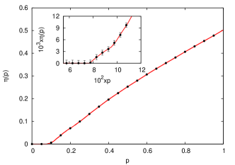
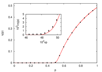
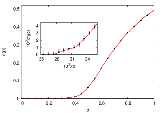
In order to validate our model, we compared the order parameter obtained from our algorithm with packet level simulations on the same network. For the comparison we used Barabási–Albert (BA) Barabási and Albert (1999), Erdős–Rényi (ER) Erdős and Rényi (1960) and Watts–Strogatz (WS) Watts and Strogatz (1998) networks. The loading probability was the same at every node of the network, and both the absorption probabilities and the elements of the transition matrix $\boldsymbol{\mathrm{P}}$ were random numbers distributed uniformly between zero and one.

The results are shown in Fig. 2. It can be seen that the theoretical curve, computed by our numerical method, fits very well to the values of the order parameter determined by simulations.

(a) BA network ($m=2$)

(b) ER network ($p_{\mathrm{ER}}=0.4$)

(c) WS network ($z=16$ and $q_{WS}=0.1024$)

Figure 2: The order parameter as a function of homogeneous loading probabilities. The graphs show numerical calculations (solid line) and particle based simulations (black points) on three distinct networks. All graphs had $N=500$ nodes. (Color online.)

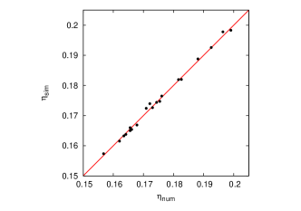
We also validated our results for inhomogeneous traffic loads. For this purpose we generated several realizations of random loading vectors, $\boldsymbol{p}$, and transition matrix $\boldsymbol{\mathrm{P}}$ on the same ER graph and compared the order parameter calculated by simulations and numerical computations. Results are shown in Fig. 3. The simulations agree with our numerical method very well.

Figure 3: Comparison of the order parameter computed numerically with our algorithm and obtained from simulation with inhomogeneous loading probabilities on an ER graph($N=500$ and $p_{ER}=0.4$). (Color online.)

IV Critical traffic load in arbitrary networks

The main difficulty of using Eq. (5) is the computational complexity of inverting the matrix $\boldsymbol{\mathrm{E}}-\boldsymbol{\mathrm{P}}$. Moreover, even if the matrix can be inverted numerically for a particular network, the dependence of the critical point on the network structure and the traffic load remains obscure. In the case of large irregular networks approximations are needed to describe the phase transition analytically.

For a detailed analysis of topological effects on the critical load $\boldsymbol{p}_{c}$, let us consider networks with random-walk-like particle transport with homogeneous absorption probabilities. In this case, if nodes $i$ and $j$ are connected in the network, the transition probability from node $i$ to node $j$ is $P_{ji}=(1-\mu)/d_{i}$, where $d_{i}$ is the degree of node $i$, and $\mu$ is the absorption probability. Using the adjacency and degree matrix of the network, $\boldsymbol{\mathrm{P}}$ can be written in a very compact form:

$$\boldsymbol{\mathrm{P}}=(1-\mu)\boldsymbol{\mathrm{A}}\boldsymbol{\mathrm{D}}^{-1}.$$ (6)

Using the spectral decomposition of the transition matrix, we can write

$$\boldsymbol{\mathrm{A}}\boldsymbol{\mathrm{D}}^{-1}=\sum_{k=1}^{N}\lambda_{k}\boldsymbol{v}_{k}\boldsymbol{w}^{T}_{k}.$$ (7)

where $\boldsymbol{w}_{k}$ and $\boldsymbol{v}_{k}$ are the left and right eigenvectors of $\boldsymbol{\mathrm{A}}\boldsymbol{\mathrm{D}}^{-1}$, respectively, and $\lambda_{k}$ is the corresponding eigenvalue. Note that the symmetric matrix $\boldsymbol{\mathrm{D}}^{-1/2}\boldsymbol{\mathrm{A}}\boldsymbol{\mathrm{D}}^{-1/2}$ has the same eigenvalue spectrum as the transition matrix $\boldsymbol{\mathrm{A}}\boldsymbol{\mathrm{D}}^{-1}$. Indeed, if $\boldsymbol{u}_{k}$ is an eigenvector of the later matrix with eigenvalue $\lambda_{k}$, then $\boldsymbol{v}_{k}=\boldsymbol{\mathrm{D}}^{1/2}\boldsymbol{u}_{k}$ will be the right, and $\boldsymbol{w}_{k}=\boldsymbol{\mathrm{D}}^{-1/2}\boldsymbol{u}_{k}$ will be the left eigenvector of $\boldsymbol{\mathrm{A}}\boldsymbol{\mathrm{D}}^{-1}$ with the same eigenvalue Lovász (1993).

The transition matrix $\boldsymbol{\mathrm{A}}\boldsymbol{\mathrm{D}}^{-1}$ is well known in the theory of random walks on graphs Lovász (1993). Its eigenvalues satisfy the inequality $-1\leq\lambda_{k}\leq 1$ Lovász (1993). The largest eigenvalue is always $\lambda_{1}=1$ and it is degenerate only if the graph is not connected. Moreover, the smallest eigenvalue is equal to $-1$ if and only if the graph is bipartite Lovász (1993). In the following we will assume that the graphs under study are connected.

It is easy to see that the normalized eigenvector of $\boldsymbol{\mathrm{D}}^{-1/2}\boldsymbol{\mathrm{A}}\boldsymbol{\mathrm{D}}^{-1/2}$ corresponding to $\lambda_{1}=1$ is $\boldsymbol{u}_{1}=\boldsymbol{\mathrm{D}}^{1/2}\boldsymbol{\mathrm{1}}/\sqrt{2M}$, where $M$ is the number of links in the network, and $\boldsymbol{\mathrm{1}}=(1,1,\dots,1)^{T}$. It follows that the left and right eigenvectors of $\boldsymbol{\mathrm{A}}\boldsymbol{\mathrm{D}}^{-1}$ corresponding to $\lambda_{1}=1$ are $\boldsymbol{w}_{1}=\boldsymbol{\mathrm{1}}^{T}/\sqrt{2M}$ and $\boldsymbol{v}_{1}=\boldsymbol{d}/\sqrt{2M}=\boldsymbol{\mathrm{D}}\boldsymbol{\mathrm{1}}/\sqrt{2M}$, respectively.

Using the power series expansion of the function $1/(1-x)$ and the spectral decomposition of the transition matrix, we can formally calculate the inverse of $\boldsymbol{\mathrm{E}}-\boldsymbol{\mathrm{P}}$:

$$(\boldsymbol{\mathrm{E}}-\boldsymbol{\mathrm{P}})^{-1}=\sum_{k=1}^{N}\frac{1}{1-(1-\mu)\lambda_{k}}\boldsymbol{v}_{k}\boldsymbol{w}^{T}_{k}.$$ (8)

The above sum can be split into three parts that have behave differently as $\mu$ is varies:

$$\sum_{\lambda_{k}=0}\boldsymbol{v}_{k}\boldsymbol{w}^{T}_{k}+\frac{1}{\mu}\frac{\boldsymbol{d}\boldsymbol{\mathrm{1}}^{T}}{2M}+\sum_{\lambda_{k}\neq 0,1}\frac{1}{1-(1-\mu)\lambda_{k}}\boldsymbol{v}_{k}\boldsymbol{w}^{T}_{k}.$$ (9)

The first term, corresponding to the eigenvalues $\lambda_{i}=0$, is independent of $\mu$. The second term, which belongs $\lambda_{1}=1$, becomes singular as $\mu\rightarrow 0$. The last term, which consists of all the eigenvalues that are neither zero nor one, is finite for every values of $\mu$.

V Discussion

V.1 Low absorption levels

In the case of low absorption levels, the second term dominates in (9). Therefore, we obtain

$$\boldsymbol{\xi}=\left(\boldsymbol{\mathrm{E}}-\boldsymbol{\mathrm{P}}\right)^{-1}\boldsymbol{p}\simeq\frac{\boldsymbol{d}}{\overline{d}}\frac{\overline{p}}{\mu},$$ (10)

where $\overline{p}=\sum_{i}p_{i}/N$ and $\overline{d}=2M/N$. Moreover, if the loading is homogeneous, i.e. $\boldsymbol{p}=p\boldsymbol{\mathrm{1}}$, the critical loading probability is

$$p_{c}=\frac{\overline{d}}{d_{\max}}\mu,$$ (11)

where $d_{\max}$ is the maximal degree in the graph.

Note that in the low absorption limit the critical point depends only on the relative spread of the degree sequence, i.e. $d_{\max}/\overline{d}$, and not on the absolute scale of the degrees. In particular, in the case of regular graphs, where each node has the same degree, the relative spread is $d_{\max}/\overline{d}=1$, so the critical point, $p_{c}=\mu$, is independent of the degree of a regular graph. Furthermore, $d_{\max}$ is always greater than or equal to $\overline{d}$, and equality holds iff the graph is regular. Therefore, the critical point $p_{c}$ is the highest in regular graphs at a given absorption level.

V.2 High absorption levels

If the absorption probability $\mu$ is close to one, then $(1-\mu)\lambda_{k}$ is close to zero, so the denominators of the third term in (9) can be approximated by one. Since the eigensystem of $\boldsymbol{\mathrm{A}}\boldsymbol{\mathrm{D}}^{-1}$ is complete, we obtain that

$$(\boldsymbol{\mathrm{E}}-\boldsymbol{\mathrm{P}})^{-1}\simeq\boldsymbol{\mathrm{E}}+\frac{1-\mu}{\mu}\frac{\boldsymbol{d}\boldsymbol{\mathrm{1}}^{T}}{2M},$$ (12)

and the state vector can be approximated by

$$\boldsymbol{\xi}\simeq\boldsymbol{p}+(1-\mu)\frac{\boldsymbol{d}}{\overline{d}}\frac{\overline{p}}{\mu}.$$ (13)

Note that we kept the $1/\mu$ factor in (13). This way Eq. (13) can reproduce Eq. (10) in the small absorption limit, since $\boldsymbol{p}$ can be neglected compared to the second term, which diverges if $\mu\rightarrow 0$.

In the case of homogeneous loading the critical loading probability is

$$p_{c}\simeq\frac{\mu}{\mu+(1-\mu)d_{\max}/\overline{d}},$$ (14)

which depends again only on $d_{\max}/\overline{d}$, the relative spread of the degree sequence. It is remarkable that the critical point is almost completely independent of the fine details of the network structure in both the small and high absorption limit.

V.3 Intermediate absorption levels

Numerical simulations presented later in this section show that Eq. (13) is valid not only for small and large values of $\mu$, but also for intermediate values if the edge density of the graph is large. The reasons are the following. The approximation that leads to Eq. (13) is the assumption that the term $(1-\mu)\lambda_{k}$ is close to zero for those $\lambda_{k}$, that are neither equal to zero nor one. This approximation is valid not only when $\mu$ is close to one, but also if the second largest absolute eigenvalue is close to zero.

If the graph is non-bipartite, the second largest absolute eigenvalue is related to $\tau$, the characteristic time until a particle reaches the stationary distribution of a random walk, as $1/\tau=\max\{|\lambda_{2}|,|\lambda_{N}|\}$. Numerical calculations, presented in Section V.4, show that $1/\tau$ decreases when the average degree increases and remains constant with small fluctuations if the average degree is fixed. Therefore, in the case of dense networks, it is plausible to use the lowest terms of the power series expansion

$$\frac{1}{1-(1-\mu)\lambda_{k}}=1+(1-\mu)\lambda_{k}+(1-\mu)^{2}\lambda_{k}^{2}+\dots.$$ (15)

in the third term of Eq. (9). The zeroth order term of the series expansion reproduces Eq. (13). If the network is not dense, like many real networks, or the absorption level is in the intermediate range we need to consider the first order term in the power series expansion (15) as well. Since bipartite and non-bipartite graphs are qualitatively different, we will discuss the two cases separately.

V.3.1 Non-bipartite graphs

It is easy to see that the first order correction to $\left(\boldsymbol{\mathrm{E}}-\boldsymbol{\mathrm{P}}\right)^{-1}$ is $(1-\mu)(\boldsymbol{\mathrm{A}}\boldsymbol{\mathrm{D}}^{-1}-\boldsymbol{d}\boldsymbol{\mathrm{1}}^{T}/2M)$. Using this correction we obtain that the state vector can approximated by

$$\boldsymbol{\xi}\simeq\boldsymbol{p}+(1-\mu)\boldsymbol{\mathrm{A}}\boldsymbol{\mathrm{D}}^{-1}\boldsymbol{p}+(1-\mu)^{2}\frac{\boldsymbol{d}}{\overline{d}}\frac{\overline{p}}{\mu}.$$ (16)

(a) The critical load, $p_{c}$, in a BA network.

(b) The critical load, $p_{c}$, in an ER network.

(c) The absolute error, $\Delta p_{c}$ in a BA network.

(d) The absolute error, $\Delta p_{c}$ in an ER network.

Figure 4: Numerical validation of the analytic results in BA ($N=512$ nodes, $m=2$) and ER ($N=64$ nodes, $p=0.1$) networks. The continuous lines $p_{c,i}$ and $p_{c,f}$ represent Eqs. (14) and (19), respectively. Numerical data, obtained by solving Eq. (5) numerically, are represented by dots. (Color online.)

In order to study the effects of the topology on the critical traffic load, let us consider homogeneous loading probabilities. After straightforward calculations we obtain that in this case the $i$th component of the state vector is

$$\frac{\xi_{i}}{p}\simeq 1+\frac{(1-\mu)^{2}}{\mu}\frac{d_{i}}{\overline{d}}+(1-\mu)\frac{d_{i}}{h_{i}}.$$ (17)

where $h_{i}$ denotes the harmonic mean of the degree of the neighbors of the $i$th node,

$$h_{i}=\left(\frac{1}{d_{i}}\sum_{j\in\mathcal{N}(i)}\frac{1}{d_{j}}\right)^{-1},$$ (18)

and $\mathcal{N}(i)$ is the set of neighbors of node $i$. Consequently, we obtain that the critical loading probability is

$$\frac{1}{p_{c}}\simeq 1+\underset{i}{\mathrm{max}}\left\{\frac{(1-\mu)^{2}}{\mu}\frac{d_{i}}{\overline{d}}+(1-\mu)\frac{d_{i}}{h_{i}}\right\},$$ (19)

which is one of the main results of our paper.

The main novelty of Eq. (19) is that it shows that the critical point of the phase transition is determined not only by the spread of the degree sequence, $d_{\max}/\overline{d}$, like in the low and high absorption limit, but also by $h_{i}$, which depends on the local structure of the network.

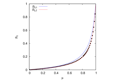
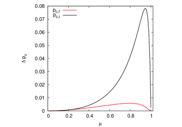
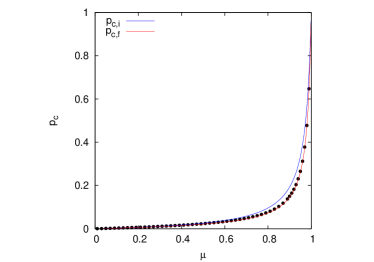
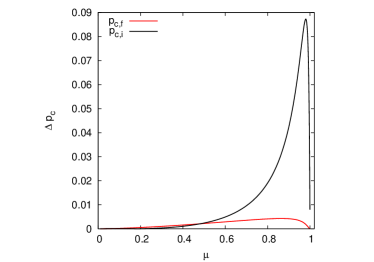
We validated our result on BA and ER networks. We calculated the critical load $p_{c}$ by inverting Eq. (5) numerically and then compared the result with Eq. (14) and Eq. (19) on the same graph with the same absorption level.

The results are presented in Fig. 4. It can be seen that the zeroth order approximation (14) is valid only for small and large absorption levels. On the contrary, the first order approximation (19) fits the numerical data closely on the whole range of absorption levels. In order to emphasize the clear advantage of Eq. (19), the absolute difference between formulas (14) and (19) and the numerical data is also shown in Fig. 4.

V.3.2 Bipartite graphs

The nodes of a bipartite graph can be divided into two disjoint groups, $\mathcal{G}_{1}$ and $\mathcal{G}_{2}$, in such a way that the edges of the graph connect only nodes from different groups. Since trees are bipartite graphs, bipartite graphs are extremely important from the practical point of view.

Suppose that there are $N_{1}$ nodes in $\mathcal{G}_{1}$ and $N_{2}$ nodes in $\mathcal{G}_{2}$, and denote the average degree and loading probability in $\mathcal{G}_{i}$ ($i=1,2$) are $\overline{d}_{i}=M/N_{i}$ and $\overline{p}_{i}=\sum_{k\in\mathcal{G}_{i}}p_{k}/N$, respectively.

The critical traffic load in bipartite graphs can be calculated similarly to the non-bipartite graphs. The calculation is based on the symmetry of the spectra of the transition matrix. Here, we only summarize the results for homogeneous loading, details of the calculation and the case of heterogeneous loading are presented in Appendix B.

In the case of a bipartite graph we obtain that each partition defines a separate critical loading probability. For low or high absorption levels and homogeneous traffic load we obtain, analogously to Eq. (14), that

$$\frac{1}{p_{c}^{(1)}}\simeq 1+\frac{1}{\mu}\frac{(1-\mu)^{2}/\overline{d}_{1}+(1-\mu)/\overline{d}_{2}}{2-\mu}d_{\max}^{(1)},$$ (20)

$$\frac{1}{p_{c}^{(2)}}\simeq 1+\frac{1}{\mu}\frac{(1-\mu)^{2}/\overline{d}_{2}+(1-\mu)/\overline{d}_{1}}{2-\mu}d_{\max}^{(2)},$$

where $d_{\max}^{(i)}$ is the maximal degree in $\mathcal{G}_{i}$. The critical loading probability of the whole network is the lesser of the two: $p_{c}=\min(p_{c}^{(1)},p_{c}^{(2)})$ .

This result is very similar to the case of non-bipartite graphs. It can be seen that $p_{c}$ depends only on the absorption level, $\mu$, and global properties of the graph, namely the mean $\overline{d}_{i}$ and the maximal degree $d_{\max}^{(i)}$, which can be obtained from the degree sequences of $\mathcal{G}_{1}$ and $\mathcal{G}_{2}$ straightforwardly.

In the case of intermediate absorption levels, the zeroth order approximation of critical traffic load, presented in (20), has to be corrected. Similarly to non-bipartite graphs, the first order correction, obtained from the spectral decomposition of the transition matrix, is proportional to $d_{i}/h_{i}$. The critical loading probabilities $p_{c}^{(1)}$ and $p_{c}^{(2)}$, including the first order corrections and corresponding to the two sub-components of a bipartite graph, are

$$\frac{1}{p_{c}^{(1)}}\simeq 1+\underset{i\in\mathcal{G}_{1}}{\mathrm{max}}\Bigg{\{} \frac{1}{\mu}\frac{(1-\mu)^{2}/\overline{d}_{1}+(1-\mu)^{3}/\overline{d}_{2}}{2-\mu}d_{i}+$$ (21)

$$+(1-\mu)d_{i}/h_{i}\Bigg{\}},$$

$$\frac{1}{p_{c}^{(2)}}\simeq 1+\underset{i\in\mathcal{G}_{2}}{\mathrm{max}}\Bigg{\{} \frac{1}{\mu}\frac{(1-\mu)^{2}/\overline{d}_{2}+(1-\mu)^{3}/\overline{d}_{1}}{2-\mu}d_{i}+$$

$$+(1-\mu)d_{i}/h_{i}\Bigg{\}}.$$

Consequently, the critical loading probability of the whole network is $p_{c}=\min\left(p_{c}^{(1)},p_{c}^{(2)}\right)$.

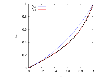
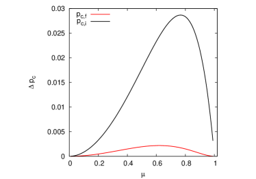
In order to validate our results, we calculated the critical load $p_{c}$ by inverting (5) numerically. For validation, we used BA scale-free trees, grown by preferential attachment, and compared the numerical data with (20) and (21) with the same graph and absorption level. The results are shown in Fig. 5. Eq. (21), which includes first order corrections, fits the numerical data closely not only at low and high absorption levels, like Eq. (20), but also in the intermediate absorption range.

(a) The critical load, $p_{c}$, as a fuction of the absorption level, $\mu$.

(b) The absolute error of the critical load, $\Delta p_{c}$, as a function of the absorption level, $\mu$.

Figure 5: Numerical validation of the analytic results on a BA tree ($N=1024$ nodes, $m=1$). The continuous lines $p_{c,i}$ and $p_{c,f}$ represent Eqs. (20) and (21), respectively. Numerical data, obtained by solving Eq. (5) numerically, are represented by dots. (Color online.)

V.4 Error estimation in the large graph limit

We have seen that in the case of non-bipartite graphs the largest absolute eigenvalue is $|\lambda_{1}|=1$, whereas in case of bipartite graphs it is $|\lambda_{1}|=|\lambda_{N}|=1$. In the power series expansion (15) we considered the largest absolute eigenvalue precisely, and neglected the higher order terms for $|\lambda|<1$. In this section we discuss the validity of our approximation, and show numerically how the precision of our model depends on the graph properties.

The error of the derived formulas depends on the magnitude of the higher order terms that we neglected in the power series expansion (15). These terms can be bounded from above with the second largest absolute eigenvalue, that is $\max\{|\lambda_{2}|,|\lambda_{N}|\}$ for non-bipartite graphs and $\lambda_{2}$ for bipartite graphs. The smaller the second largest absolute eigenvalues are, the smaller the error of Eq. (19) and Eq. (21) is.

Although it is easy to manipulate the eigenvalues $\lambda_{k}$ formally, it is difficult to see how the eigenvalues depend on the graph properties. In order to see more easily how the error depends on the graph properties, let us introduce the mixing time from the theory of random walk on graphs.

The mixing time, $\tau$, is the expected time until a particle, performing random walk on a graph, reaches a stationary distribution. It can be shown that the mixing rate, the reciprocal of the mixing time, is precisely equal to the second largest eigenvalue, i.e. $1/\tau=\max\{|\lambda_{2}|,|\lambda_{N}|\}$ for non-bipartite graphs and $1/\tau=\lambda_{2}$ for bipartite graphs Lovász (1993). Therefore, it is plausible to conclude that for graphs which have small mixing rate, the error will be also small.

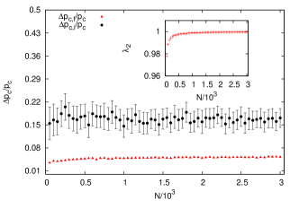
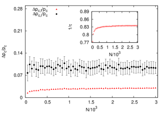
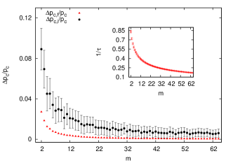
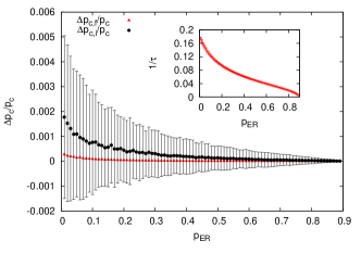
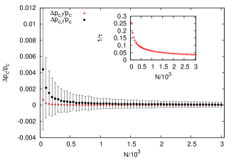
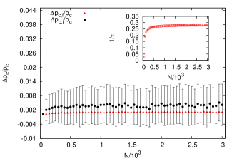
There is no known formula in the literature on how the mixing rate depends on the graph parameters in general Lovász . However, our numerical experiments showed that the mixing rate depends strongly on the edge density, $M/N=\overline{d}/2$. In particular the mixing rate decreases as the edge density increases. In Fig. 7 we can see the relative error of the derived formulas, $\Delta p_{c}/p_{c}$, as the function of various graph parameters. In the inset we can see the mixing rate as the function of the corresponding graph parameter.

In the case of a BA network, for example, the edge density is $M/N\simeq m$, where $m$ is the number of edges connecting the new nodes to the graph in preferential attachment. This means that the mixing rate, $1/\tau$, remains constant with small fluctuations if $m$ is fixed, even if $N\to\infty$. This phenomenon is the same in bipartite and non-bipartite graphs. For example, one obtains a BA scale-free tree, which is a bipartite graph, if $m\equiv 1$, In this case the error of the derived formulas is also constant, and it will not decrease even in the thermodynamic limit.

In Fig. 6(a) and Fig. 6(b) we can see BA networks with $m=1$ and $m=2$ fixed, and $N$ varied. These cases correspond to a bipartite and a non-bipartite graph, respectively. We can see that in both cases both the relative error and the mixing rate tends to a fixed value as $N\to\infty$. On the other hand, in Fig. 6(c) the size of the graph is fixed, and $m$ is varied. We can see that the mixing rate increases as $m$ increases and, at the same time, the relative tends to zero.

The construction of ER networks is fundamentally different from the BA graphs. In the case of ER networks, the edge density is $M/N=p(N-1)/2\simeq pN/2$. Therefore, the edge density increases, and the relative error tends to zero, if either $p$ or $N$ is increased, and the other parameter is fixed. Note that in case of $p=1$ the ER network is a complete graph, in which case the derived formulas are exact. In contrast, the relative error of the derived formulas tends to a fixed value if $pN$ is fixed.

Numerical simulations carried out on ER networks are shown in Fig. 7. We can see that the simulation results confirm our assumption that the relative error of the derived formulas decreases if the density of the network increases, and remain fixed if the density is fixed.

(a) BA tree with $m=1$ fixed and $N$ varied.

(b) BA network with $m=2$ fixed and $N$ varied.

(c) BA network with $N=1024$ fixed and $m$ varied.

Figure 6: The relative error, $\Delta p_{c}/p_{c}$, of the derived formulas as a function of $N$ and $m$ in BA networks with absorption rate $\mu=0.8$. The black dots and red triangles show the error of the derived zeroth and first order approximations, respectively. The insets show the dependence of the mixing rate, $1/\tau$ on $N$ and $m$. Data points were averaged over $32$ graph realization in each case. (Color online.)

(a) ER network with $N=1024$ fixed and $p_{ER}$ varied.

(b) ER network with $p_{ER}=0.5$ fixed and $N$ varied.

(c) ER with $Np_{ER}=49$ fixed and $N$ varied.

Figure 7: The relative error, $\Delta p_{c}/p_{c}$, of the derived formulas as a function of $N$ and $p_{ER}$ in ER networks with absorption rate $\mu=0.8$ (Figs. 7(a) and 7(b)) and $\mu=0.5$ (Fig. 7(c)). The black points and red triangles show the error of the derived zeroth and first order approximation, respectively. The insets show the dependence of the mixing rate, $1/\tau$, on $N$ and $p_{ER}$. Data points were averaged over $32$ graph realizations in each case. (Color online.)

VI Conclusion

In this paper, we studied congestion phenomena in queuing networks. We analyzed how the critical point of the phase transition between free and congested phases is influenced by the topological properties of the network. In order to study the influence of the network structure on the traffic dynamics in an arbitrary network, we neglected congestion control mechanisms, and we modeled the particle transport by a simple Markovian random walk.

In our model the critical traffic load in the network can be controlled by the absorption level of the particles. We first derived Eq. (14), the zeroth order approximation for the critical traffic load for low and high absorption levels. This result has been obtained by De Martino et al De Martino et al. (2009a) on a model with a congestion control mechanism included. Our result confirms their finding that at the critical point the details of the congestion control mechanism are less important in some cases.

In our paper we also showed that in the case of intermediate absorption levels the zeroth order formula is not valid, and higher order corrections are needed. We derived Eq. (19) which incorporates the first order corrections to Eq. (14) and improves the precision of the critical point considerably. In contrast to the zeroth order formula, higher order corrections include not only the global properties of the degree sequence, i.e. the mean and maximum degree, but also the local information on the network structure. The improvement achieved by the higher order correction was validated by numerical simulations.

We also demonstrated that in the case of intermediate absorption levels the structure of the network can have dramatic effects on the analytic behavior of the critical point. We showed, in particular, that one must pay special attention when considering a bipartite graph, because the spectra of bipartite graphs are symmetrical. We derived Eq. (21) and showed that the critical point in a bipartite graph is the maximum of the critical points of its sub-components.

Finally, we investigated the validity of our model. We showed that the higher order terms that were neglected during our calculations depend on the spectral gap, which can also be expressed by the mixing rate in the graph. We presented numerical arguments that the mixing ratio, that is the precision of our approximations, strongly depends on the edge density $M/N$. This empirical fact is well known in the mathematical community, but up to now, as far as we know, there is no rigorous proof of the phenomenon. We would like to examine this question in detail in our future work.

VII Acknowledgements

This work was partially supported by the National Science Foundation OTKA 7779, the National Development Agency (TAMOP 4.2.1/B-09/1/KMR-2010-0003) and the EU FIRE NOVI project (Grant No. 257867). We are also grateful to professor László Lovász for the useful discussions on the mixing rate of graphs.

Appendix A

Let us suppose that $\boldsymbol{\mathrm{E}}-\boldsymbol{\mathrm{P}}$ is not invertible, which is equivalent to the statement that $\boldsymbol{\mathrm{P}}$ has a normalized eigenvector $\boldsymbol{x}$ with eigenvalue $1$. In this case, using the assumption that there is at least one node where $\sum_{i}P_{ij}<1$ (e.i. there is absorption at least at one node), the following inequalities will hold:

$$\sum_{i=1}^{N}|x_{i}|\leq\sum_{j=1}^{N}\sum_{i=1}^{N}P_{ij}|x_{j}|<\sum_{j=1}^{N}|x_{j}|,$$ (22)

which is a contradiction.

Appendix B

Using an indexing of the nodes that is suitable for the definition of bipartite graphs, every vector mentioned in the main text can be split into two parts, $\boldsymbol{p}=(\boldsymbol{p}_{1},\boldsymbol{p}_{2})^{T}$, $\boldsymbol{d}=(\boldsymbol{d}_{1},\boldsymbol{d}_{2})^{T}$ $\boldsymbol{\xi}=(\boldsymbol{\xi}_{1},\boldsymbol{\xi}_{2})^{T}$ such that the $N_{1}$ ($N_{2}$) components of the first (second) part belong to nodes in $\mathcal{G}_{1}$ ($\mathcal{G}_{2}$). The form of $\boldsymbol{\mathrm{A}}$ and $\boldsymbol{\mathrm{D}}$ are the following.

$$\boldsymbol{\mathrm{A}}=\begin{pmatrix}\boldsymbol{0}&\boldsymbol{\mathrm{B}}\\ \boldsymbol{\mathrm{B}}^{T}&\boldsymbol{0}\end{pmatrix}\quad\boldsymbol{\mathrm{D}}=\begin{pmatrix}\boldsymbol{\mathrm{D}}_{1}&\boldsymbol{0}\\ \boldsymbol{0}&\boldsymbol{\mathrm{D}}_{2}\end{pmatrix},$$ (23)

where $\boldsymbol{\mathrm{B}}$ is an $N_{1}\times N_{2}$, $\boldsymbol{\mathrm{D}}_{1}$ is an $N_{1}\times N_{1}$ and $\boldsymbol{\mathrm{D}}_{2}$ is an $N_{2}\times N_{2}$ matrix. The transition matrix has the following form:

$$\boldsymbol{\mathrm{A}}\boldsymbol{\mathrm{D}}^{-1}=\begin{pmatrix}\boldsymbol{0}&\boldsymbol{\mathrm{B}}\boldsymbol{\mathrm{D}}_{2}^{-1}\\ \boldsymbol{\mathrm{B}}^{T}\boldsymbol{\mathrm{D}}_{1}^{-1}&\boldsymbol{0}\end{pmatrix}$$ (24)

The structure of $\boldsymbol{\mathrm{D}}^{-1/2}\boldsymbol{\mathrm{A}}\boldsymbol{\mathrm{D}}^{-1/2}$ is similar to $\boldsymbol{\mathrm{A}}$, the off-diagonal block matrices are $\boldsymbol{\mathrm{D}}_{1}^{-1/2}\boldsymbol{\mathrm{B}}\boldsymbol{\mathrm{D}}_{2}^{-1/2}$ and its transpose. A one line calculation shows, that if $\boldsymbol{u}_{i}=(\boldsymbol{u}_{1,k},\boldsymbol{u}_{2,k})^{T}$ is an eigenvector of $\boldsymbol{\mathrm{D}}^{-1/2}\boldsymbol{\mathrm{A}}\boldsymbol{\mathrm{D}}^{-1/2}$ with eigenvalue $\lambda_{k}$, then the vector $(\boldsymbol{u}_{1,k},-\boldsymbol{u}_{2,k})^{T}$, is also an eigenvector with eigenvalue $-\lambda_{k}$, so the spectra of $\boldsymbol{\mathrm{D}}^{-1/2}\boldsymbol{\mathrm{A}}\boldsymbol{\mathrm{D}}^{-1/2}$ is symmetric to the origin. One consequence of this symmetry is that if the number of nodes is even (odd), the kernel dimension of $\boldsymbol{\mathrm{D}}^{-1/2}\boldsymbol{\mathrm{A}}\boldsymbol{\mathrm{D}}^{-1/2}$ is also even (odd). For the sake of simplicity, we study only bipartite graphs with an even number of nodes. For large networks, this has no serious consequence. Let us define the matrices $\boldsymbol{\mathrm{I}}^{(1)}_{k}$ and $\boldsymbol{\mathrm{I}}^{(2)}_{k}$:

$$\boldsymbol{\mathrm{I}}^{(1)}_{k}=\begin{pmatrix}\boldsymbol{u}_{1,k}\boldsymbol{u}_{1,k}^{T}&\boldsymbol{0}\\ \boldsymbol{0}&\boldsymbol{u}_{2,k}\boldsymbol{u}_{2,k}^{T}\end{pmatrix},$$ (25)

and

$$\boldsymbol{\mathrm{I}}^{(2)}_{k}=\begin{pmatrix}\boldsymbol{0}&\boldsymbol{u}_{1,k}\boldsymbol{u}_{2,k}^{T}\\ \boldsymbol{u}_{2,k}\boldsymbol{u}_{1,k}^{T}&\boldsymbol{0}\end{pmatrix}.$$ (26)

Then, the spectral decomposition of $\boldsymbol{\mathrm{D}}^{-1/2}\boldsymbol{\mathrm{A}}\boldsymbol{\mathrm{D}}^{-1/2}$ is

$$\sum_{k=1}^{N}\lambda_{k}(\boldsymbol{\mathrm{I}}^{(1)}_{k}+\boldsymbol{\mathrm{I}}^{(2)}_{k})=\sum_{k=1}^{N/2}2\lambda_{k}\boldsymbol{\mathrm{I}}^{(2)}_{k}$$ (27)

It is easier to perform the calculation on the spectral decomposition of $\boldsymbol{\mathrm{D}}^{-1/2}\boldsymbol{\mathrm{A}}\boldsymbol{\mathrm{D}}^{-1/2}$ instead of $\boldsymbol{\mathrm{A}}\boldsymbol{\mathrm{D}}^{-1}$ to get an approximation of $(\boldsymbol{\mathrm{E}}-\boldsymbol{\mathrm{P}})^{-1}$:

$$(\boldsymbol{\mathrm{E}}-\boldsymbol{\mathrm{P}})^{-1}=\boldsymbol{\mathrm{D}}^{1/2}(\boldsymbol{\mathrm{E}}-(1-\mu)\boldsymbol{\mathrm{D}}^{-1/2}\boldsymbol{\mathrm{A}}\boldsymbol{\mathrm{D}}^{-1/2})^{-1}\boldsymbol{\mathrm{D}}^{-1/2}.$$ (28)

The spectral decomposition of the factor in the middle of the r. h. s.  is

$$\sum_{k=1}^{N}\frac{\boldsymbol{u}_{k}\boldsymbol{u}_{k}^{T}}{1-(1-\mu)\lambda_{i}},$$ (29)

which, using the symmetry of the spectra, can be written in the form

$$\sum_{k=1}^{N/2}2\frac{\boldsymbol{\mathrm{I}}^{(1)}_{k}+(1-\mu)\lambda_{k}\boldsymbol{\mathrm{I}}^{(2)}_{k}}{1-(1-\mu)^{2}\lambda_{k}^{2}}.$$ (30)

This also can be split into three parts as in 9:

$$\sum_{\lambda_{k}=0}2\boldsymbol{\mathrm{I}}^{(1)}_{k} +\frac{2}{\mu}\frac{\boldsymbol{\mathrm{I}}^{(1)}_{k}+(1-\mu)\boldsymbol{\mathrm{I}}^{(2)}_{k}}{2-\mu}+$$ (31)

$$+\sum_{\lambda_{k}\neq 0,1}2\frac{\boldsymbol{\mathrm{I}}^{(1)}_{k}+(1-\mu)\lambda_{k}\boldsymbol{\mathrm{I}}^{(2)}_{k}}{1-(1-\mu)^{2}\lambda_{k}^{2}},$$

but here, summation runs over only the first half of the spectra. The power series expansion of the summands of the last term is

$$2\boldsymbol{\mathrm{I}}^{(1)}_{k}+2(1-\mu)\lambda_{k}\boldsymbol{\mathrm{I}}^{(2)}_{k}+2(1-\mu)^{2}\lambda^{2}_{k}\boldsymbol{\mathrm{I}}^{(1)}_{k}+\dots$$ (32)

Dropping all the terms except the first gives

$$\boldsymbol{\mathrm{E}}+\frac{2}{\mu}\frac{(1-\mu)^{2}\boldsymbol{\mathrm{I}}^{(1)}_{1}+(1-\mu)\boldsymbol{\mathrm{I}}^{(2)}_{1}}{2-\mu}$$ (33)

as the inverse of $\boldsymbol{\mathrm{E}}-(1-\mu)\boldsymbol{\mathrm{D}}^{-1/2}\boldsymbol{\mathrm{A}}\boldsymbol{\mathrm{D}}^{-1/2}$, so

$$(\boldsymbol{\mathrm{E}}-\boldsymbol{\mathrm{P}})^{-1}\simeq\boldsymbol{\mathrm{E}}+\frac{1}{\mu}\frac{(1-\mu)^{2}\boldsymbol{\mathrm{J}}^{(1)}_{1}+(1-\mu)\boldsymbol{\mathrm{J}}^{(2)}_{1}}{2-\mu},$$ (34)

where $\boldsymbol{\mathrm{J}}^{(1)}_{1}$ and $\boldsymbol{\mathrm{J}}^{(2)}_{1}$ are the following matrices:

$$\boldsymbol{\mathrm{J}}^{(1)}_{1}=\frac{1}{M}\begin{pmatrix}\boldsymbol{d}_{1}\boldsymbol{\mathrm{1}}_{1}^{T}&\boldsymbol{0}\\ \boldsymbol{0}&\boldsymbol{d}_{2}\boldsymbol{\mathrm{1}}_{2}^{T}\end{pmatrix},$$ (35)

and

$$\boldsymbol{\mathrm{J}}^{(2)}_{1}=\frac{1}{M}\begin{pmatrix}\boldsymbol{0}&\boldsymbol{d}_{1}\boldsymbol{\mathrm{1}}_{2}^{T}\\ \boldsymbol{d}_{2}\boldsymbol{\mathrm{1}}_{1}^{T}&\boldsymbol{0}\end{pmatrix}.$$ (36)

This gives the values of $\boldsymbol{\xi}_{1}$ and $\boldsymbol{\xi}_{2}$:

$$\boldsymbol{\xi}_{1} =\boldsymbol{p}_{1}+\frac{1}{\mu}\frac{(1-\mu)^{2}\overline{p}_{1}/\overline{d}_{1}+(1-\mu)\overline{p}_{2}/\overline{d}_{2}}{2-\mu}\boldsymbol{d}_{1},$$ (37)

$$\boldsymbol{\xi}_{2} =\boldsymbol{p}_{2}+\frac{1}{\mu}\frac{(1-\mu)^{2}\overline{p}_{2}/\overline{d}_{2}+(1-\mu)\overline{p}_{1}/\overline{d}_{1}}{2-\mu}\boldsymbol{d}_{2}.$$

Eq. 20 gives the final result for homogeneous loading.

To get the first finite size correction, we have to use not only the first, but also the second term in 32. Using Eq. 27, the correction term to the inverse of $\boldsymbol{\mathrm{E}}-(1-\mu)\boldsymbol{\mathrm{D}}^{-1/2}\boldsymbol{\mathrm{A}}\boldsymbol{\mathrm{D}}^{-1/2}$ appears to be $(1-\mu)\boldsymbol{\mathrm{D}}^{-1/2}\boldsymbol{\mathrm{A}}\boldsymbol{\mathrm{D}}^{-1/2}-2(1-\mu)\boldsymbol{\mathrm{I}}^{(2)}_{1}$, so the corrected formula for the inverse is

$$\boldsymbol{\mathrm{E}} +\frac{2}{\mu}\frac{(1-\mu)^{2}\boldsymbol{\mathrm{I}}^{(1)}_{1}+(1-\mu)^{3}\boldsymbol{\mathrm{I}}^{(2)}_{1}}{2-\mu}+$$ (38)

$$+(1-\mu)\boldsymbol{\mathrm{D}}^{-1/2}\boldsymbol{\mathrm{A}}\boldsymbol{\mathrm{D}}^{-1/2},$$

and the inverse of $\boldsymbol{\mathrm{E}}-\boldsymbol{\mathrm{P}}$ is

$$(\boldsymbol{\mathrm{E}}-\boldsymbol{\mathrm{P}})^{-1}\simeq\boldsymbol{\mathrm{E}} +\frac{1}{\mu}\frac{(1-\mu)^{2}\boldsymbol{\mathrm{J}}^{(1)}_{1}+(1-\mu)^{3}\boldsymbol{\mathrm{J}}^{(2)}_{1}}{2-\mu}$$ (39)

$$+(1-\mu)\boldsymbol{\mathrm{A}}\boldsymbol{\mathrm{D}}^{-1}.$$

The corrected values of $\boldsymbol{\xi}_{1}$ and $\boldsymbol{\xi}_{2}$ are

$$\boldsymbol{\xi}_{1}\simeq\boldsymbol{p}_{1} +\frac{1}{\mu}\frac{(1-\mu)^{2}\overline{p}_{1}/\overline{d}_{1}+(1-\mu)^{3}\overline{p}_{2}/\overline{d}_{2}}{2-\mu}\boldsymbol{d}_{1}+$$ (40)

$$+(1-\mu)\boldsymbol{\mathrm{B}}\boldsymbol{\mathrm{D}}_{2}^{-1}\boldsymbol{\mathrm{1}}_{1}$$

$$\boldsymbol{\xi}_{2}\simeq\boldsymbol{p}_{2} +\frac{1}{\mu}\frac{(1-\mu)^{2}\overline{p}_{2}/\overline{d}_{2}+(1-\mu)^{3}\overline{p}_{1}/\overline{d}_{1}}{2-\mu}\boldsymbol{d}_{2}+$$

$$+(1-\mu)\boldsymbol{\mathrm{B}}^{T}\boldsymbol{\mathrm{D}}_{1}^{-1}\boldsymbol{\mathrm{1}}_{2}$$

In the case of homogeneous loading probabilities, this leads to the appearance of the harmonic means:

$$\frac{\xi_{1,i}}{p}\simeq 1 +\frac{1}{\mu}\frac{(1-\mu)^{2}/\overline{d}_{1}+(1-\mu)^{3}/\overline{d}_{2}}{2-\mu}+$$ (41)

$$+(1-\mu)d_{i}/h_{i},$$

$$\frac{\xi_{2,i}}{p}\simeq 1 +\frac{1}{\mu}\frac{(1-\mu)^{2}/\overline{d}_{2}+(1-\mu)^{3}/\overline{d}_{1}}{2-\mu}d_{i}+$$

$$+(1-\mu)d_{i}/h_{i},$$

and the individual critical loading probabilities in $\mathcal{G}_{1}$ and $\mathcal{G}_{2}$ are those that are in Eq. 21.

Appendix C

The following algorithm calculates the order parameter. Suppose that $\boldsymbol{p}=p\boldsymbol{e}$, where $\boldsymbol{e}$ is a normalized vector. If $p$ is close to zero, the network is in the uncongested phase, the components of $\boldsymbol{\xi}(p)$ satisfy Eq. 5 and the number of the uncongested nodes is equal to the number of the nodes in the system. If one increases $p$ slowly, one finds that one or more nodes will surely have at least one waiting particle in their queues in the stationary regime, i. e. at least one $\xi_{i}(p)$ becomes $1$ at a certain value of $p$. Increasing $p$ toward this value drives these nodes to the congested state, and the expected value of the growing length at the queues at these nodes in one time step is $pe_{i}+\sum_{j}P_{ij}-1$. On the other hand, these congested nodes send particles to their neighbors with rates equal to the corresponding element of $\boldsymbol{\mathrm{P}}$. These ideas suggest the following algorithm.

1. Set $\boldsymbol{\mathrm{P}}^{(0)}=\boldsymbol{\mathrm{P}}$, $\boldsymbol{y}^{(0)}=\boldsymbol{e}$, $\boldsymbol{z}^{(0)}=\boldsymbol{0}$ and $s$ to a small positive number.

2. In the $k$th step, calculate the vector

   $$\boldsymbol{x}^{(k)}(s)=(\boldsymbol{\mathrm{E}}^{(k)}-\boldsymbol{\mathrm{P}}^{(k)})^{-1}(s\boldsymbol{y}^{(k)}+\boldsymbol{z}^{(k)}).$$ (42)

   Starting from the last value at the $(k-1)$th step, increase $s$ until one of the components of $\boldsymbol{x}^{(k)}$ becomes $1$, or $s$ becomes $p$. If the latter is the case, equate the components of $\boldsymbol{\xi}$ to the corresponding components of $\boldsymbol{x}^{(k)}$. If the former is true, set $\xi_{i}=1$ at the node where $x^{(k)}_{i}$ is equal to one - this is the new congested node. Increase every component of $\boldsymbol{z}^{(k)}$ with the corresponding element of $\boldsymbol{\mathrm{P}}$ located in the column of the new congested node. Delete the rows and columns of the new congested node in $\boldsymbol{\mathrm{E}}^{(k)}$, $\boldsymbol{\mathrm{P}}^{(k)}$, $\boldsymbol{x}^{(k)}$ and $\boldsymbol{z}^{(k)}$ . This gives matrices $\boldsymbol{\mathrm{E}}^{(k+1)}$, $\boldsymbol{\mathrm{P}}^{(k+1)}$ and vectors $\boldsymbol{x}^{(k+1)}$ and $\boldsymbol{z}^{(k+1)}$ for the $(k+1)$th step.

3. If all components of $\boldsymbol{\xi}$ are calculated, the order parameter is

   $$\eta(\boldsymbol{p})=\frac{\sum_{\xi_{i}=1}\left(p_{i}+\sum_{j}P_{ij}\xi_{j}-1\right)}{\sum_{i}p_{i}}.$$ (43)

References

- De Martino et al. (2009a) D. De Martino, L. Dall’Asta, G. Bianconi, and M. Marsili, J. Stat. Mech. 2009, 08023 (2009a).
- De Martino et al. (2009b) D. De Martino, L. Dall’Asta, G. Bianconi, and M. Marsili, Phys. Rev. E 79, 015101 (2009b).
- Albert and Barabási (2002) R. Albert and A.-L. Barabási, Rev. Mod. Phys. 74, 47 (2002).
- Newman (2003) Newman, SIAM Review 45, 167 (2003).
- Ohira and Sawatari (1998) T. Ohira and R. Sawatari, Phys. Rev. E 58, 193 (1998).
- Arenas et al. (2001) A. Arenas, A. D. az Guilera, and R. Guimerà, Phys. Rev. Lett. 86, 3196 (2001).
- Zhao et al. (2005a) L. Zhao, Y.-C. Lai, K. Park, and N. Ye, Phys. Rev. E 71, 026125 (2005a).
- Echenique et al. (2005) P. Echenique, J. Gómez-Gardeñes, and Y. Moreno, Europhys. Lett. 71, 325 (2005).
- Meloni and Gómez-Gardeñes (2010) S. Meloni and J. Gómez-Gardeñes, Phys. Rev. E 82, 056105 (2010).
- Ling et al. (2009) X. Ling, M.-B. Hu, R. Jiang, R. Wang, X.-B. Cao, and Q.-S. Wu, Phys. Rev. E 80, 066110 (2009).
- Ling et al. (2010) X. Ling, M.-B. Hu, R. Jiang, and Q.-S. Wu, Phys. Rev. E 81, 016113 (2010).
- Tretyakov et al. (1998) A. Y. Tretyakov, H. Takayasu, and M. Takayasu, Physica A 253, 315 (1998).
- Strogatz (2001) S. H. Strogatz, Nature 410, 268 (2001).
- Dorogovtsev et al. (2008) S. N. Dorogovtsev, A. V. Goltsev, and J. F. F. Mendes, Rev. Mod. Phys. 80, 1275 (2008).
- Boccaletti et al. (2006) S. Boccaletti, V. Latora, Y. Moreno, M. Chavez, and D.-U. Hwang, Physics Reports 424, 175 (2006).
- Mukherjee and Manna (2005) G. Mukherjee and S. S. Manna, Phys. Rev. E 71, 066108 (2005).
- Chung (1997) F. R. K. Chung, Spectral Graph Theory (American Mathematical Society, 1997).
- Bolch et al. (2006) L. Bolch, S. Greiner, H. de Meer, and K. Trivedi, Queueing networks and Markov chains (Wiley Interscience, 2006).
- Bhat (2008) U. Bhat, An Introduction to Queueing Theory (Wiley Interscience, 2008).
- Guimerà et al. (2002) R. Guimerà, A. Díaz-Guilera, F. Vega-Redondo, A. Cabrales, and A. Arenas, Phys. Rev. Lett. 89, 248701 (2002).
- Hu et al. (2007) M.-B. Hu, W.-X. Wang, R. Jiang, Q.-S. Wu, and Y.-H. Wu, Phys. Rev. E 75, 036102 (2007).
- Zhao et al. (2005b) L. Zhao, Y.-C. Lai, K. Park, and N. Ye, Phys. Rev. E 71, 026125 (2005b).
- Zhang et al. (2007) H. Zhang, Z. Liu, M. Tang, and P. Hui, Phys. Lett. A 364, 177 (2007).
- Takayasu et al. (1996) M. Takayasu, H. Takayasu, and K. Fukuda, Physica A 233, 824 (1996).
- Takayasu et al. (2000) M. Takayasu, H. Takayasu, and K. Fukuda, Physica A 277, 248 (2000).
- Barabási and Albert (1999) A.-L. Barabási and R. Albert, Science 286, 509 (1999).
- Erdős and Rényi (1960) P. Erdős and A. Rényi, Publ. Math. Inst. Hung. Acad. Sci. 5, 17 (1960).
- Watts and Strogatz (1998) D. J. Watts and S. H. Strogatz, Nature 393, 440 (1998).
- Lovász (1993) L. Lovász, in Combinatorics, Paul Erdős is Eighty, Vol. 2 (Bolyai Society, 1993).
- (30) L. Lovász, Private communication.