Simple Asymmetric Exclusion Model and Lattice Paths: Bijections and Involutions

Abstract

We study the combinatorics of the change of basis of three representations of the stationary state algebra of the two parameter simple asymmetric exclusion process. Each of the representations considered correspond to a different set of weighted lattice paths which, when summed over, give the stationary state probability distribution. We show that all three sets of paths are combinatorially related via sequences of bijections and sign reversing involutions.

Short title: ASEP and Lattice Paths: Bijections and Involutions

PACS numbers: 05.50.+q, 05.70.fh, 61.41.+e

Key words: Asymmetric Simple Exclusion Process, combinatorial representations, basis change, lattice paths.

1 Introduction

The Simple Asymmetric Exclusion Process (ASEP) is a stochastic process defined by particles hopping along a line of length $L$ – see Figure 1. Particles hop on to the line on the left with probability $\alpha$, off at the right with probability $\beta$ and between vertices to the right with unit probability with the constraint that only one particle can occupy a vertex.

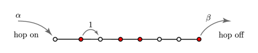
Figure 1: ASEP hopping model

The problem of readily computing the stationary probability distribution was solved by Derrida et al [6] with the introduction of the “matrix product” Ansatz (see below) which provides an algebraic method of computing the stationary distribution. The ASEP and variations of it are a rich source of combinatorics: progress has been made in understanding the stationary distribution purely combinatorially [5, 7, 8] and computing the stationary distribution has been shown to be equivalent to solving various lattice path problems [4] or permutation tableaux [10]. A recent review of the Asymmetric Exclusion Process may be found in Blythe and Evans [1].

As explained in detail below, the matrix product Ansatz expresses the stationary distribution of a given state as a matrix product (the exact form of the product depends on the state). The matrices arise as representations of the DEHP algebra. The paper by Derrida et al [6] originally found three different representations. As shown by Brak and Essam [4], each matrix representation can be interpreted as a transfer matrix (see [9] section 4.7) for a different lattice path model. Computing the stationary distribution is thus translated into finding certain lattice path weight polynomials.

Each of the three lattice path models are quite different (see - Figure 2) however they all have the same weight polynomials (as they must since they all correspond to the same stationary probability). Our primary interest in this paper is to shown how this arises combinatorially. This will be done by showing that all three path models are related by weight preserving bijections and involutions. Rather than enunciate the three possible connections between the three paths we rather show how they biject to a fourth “canonical” path model – see Figure 2.

The primary consequences of theses connections are two-fold. Firstly the canonical path model provides a new representation of the DEHP algebra and secondly, since each of these lattice paths arise from representations of the DEHP algebra the bijections between the different representations correspond algebraically to similarity transformations between the representations. Although we don’t do so in this paper, it would be interesting to see how (if at all) the bijections are related to the similarity matrices themselves.

An additional interest of the canonical path model is that it can be interpreted as an interface polymer model. This polymer model has recently been used [2] to gain a new understanding of how equilibrium models in statistical mechanics are imbedded in non-equilibrium process.

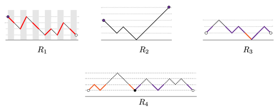
Figure 2: The lattice path models associated with the three algebra representations and the $R_{4}$, ‘canonical’ representation path.

2 Markov chain and ASEP algebra

We now define the ASEP and briefly explain the Matrix product Anstaz. The state of the chain, $\mathbf{\tau}=(\tau_{1},\dots,\tau_{L})\in(0,1)^{L}$, is determined by the particle occupancy

$$\tau_{i}=\begin{cases}1&\text{if vertex $i$ is occupied}\\ 0&\text{otherwise}\end{cases}$$ (2.1)

The transition matrix, $\mathcal{P}$ has elements,

• Hopping on: $\mathcal{P}\left((0,\dots,\tau_{L},),(1,\dots,\tau_{L})\right)=\alpha$

• Hopping off: $\mathcal{P}\left((\tau_{1},\dots,\tau_{L-1},1),(\tau_{1},\dots,\tau_{L-1},0)\right)=\beta$

• Right hopping: $\mathcal{P}\left((\tau_{1},\dots,\tau_{i},\dots,\tau_{L}),(\tau_{1},\dots,1-\tau_{i},\dots,\tau_{L})\right)=1$, for $\tau_{i}=1$, $1\leq i<L$.

All other elements of $\mathcal{P}$ are zero except the diagonals for which $\mathcal{P}(\tau,\tau)=1-\sum_{\tau^{\prime}\in(0,1)^{L},\tau^{\prime}\neq\tau}\mathcal{P}(\tau^{\prime},\tau)$ The primary object we wish to determine is the stationary state vector $\vec{P}_{S}$ determined by
$\mathcal{P}\vec{P}_{S}=0$. Derrida et al[6], have shown that the stationary state vector could be written as a matrix product Ansatz, in particular they show the following.

Theorem 1.

[6] Let $D$ and $E$ be matrices then the components of the stationary state vector are given by

$$P_{S}(\tau)=\frac{1}{Z_{L}}\,W\,\left[\prod_{i=1}^{L}(\tau_{i}D+(1-\tau_{i})E)\right]\,V$$ (2.2)

with normalisation $Z_{L}$ given by

$$Z_{L}=W(DE)^{L}V$$ (2.3)

provided that $D$ and $E$ satisfy the DEHP algebra

$$D+E =DE$$ (2.4a)

and $$W V$$ and are the left and right eigenvectors

$$WE =\frac{1}{\alpha}W,\qquad DV=\frac{1}{\beta}V.$$ (2.4b)

These equations are sufficient to determine $P_{S}(\tau)$ algebraically. Derrida et al [6] also gave several matrix representations of $D$ and $E$ and the vectors $|V\rangle$ and $\langle W|$, any one of which may also used to determine $P_{S}(\tau)$.

The three representations found by Derrida et al [6] are conveniently expressed in terms if the variables

$$\bar{\alpha} =1/\alpha$$ (2.5a)

$$\bar{\beta} =1/\beta$$ (2.5b)

$$c =\bar{\alpha}-1$$ (2.5c)

$$d =\bar{\beta}-1$$ (2.5d)

$$\kappa^{2} =\bar{\alpha}+\bar{\beta}-\bar{\alpha}\bar{\beta}=1-cd$$ (2.5e)

and are as follows.

Representation I

$$D_{1}=\begin{pmatrix}\bar{\beta}&\bar{\beta}&\bar{\beta}&\bar{\beta}&\bar{\beta}&\cdots\\ 0&1&1&1&1&\cdots\\ 0&0&1&1&1&\cdots\\ 0&0&0&1&1&\cdots\\ \vdots&\vdots&\vdots&\vdots&\end{pmatrix}\qquad E_{1}=\begin{pmatrix}0&0&0&0&0&\cdots\\ 1&0&0&0&0&\cdots\\ 0&1&0&0&0&\cdots\\ 0&0&1&0&0&\cdots\\ \vdots&\vdots&\vdots&\vdots&\end{pmatrix}$$ (2.6)

$$W_{1}=(1,\bar{\alpha},\bar{\alpha}^{2},\bar{\alpha}^{3},\ldots)\qquad V_{1}=(1,0,0,0,\ldots)^{T}$$ (2.7)

Representation II

$$D_{2}=\begin{pmatrix}1&1&0&0&0&\cdots\\ 0&1&1&0&0&\cdots\\ 0&0&1&1&0&\cdots\\ 0&0&0&1&1&\cdots\\ \vdots&\vdots&\vdots&\vdots&\end{pmatrix}\qquad E_{2}=\begin{pmatrix}1&0&0&0&0&\cdots\\ 1&1&0&0&0&\cdots\\ 0&1&1&0&0&\cdots\\ 0&0&1&1&0&\cdots\\ \vdots&\vdots&\vdots&\vdots&\end{pmatrix}$$ (2.8)

$$W_{2}=\kappa(1,c,c^{2},c^{3},\ldots)\qquad V_{2}=\kappa(1,d,d^{2},d^{3},\ldots)^{T}$$ (2.9)

Representation III

$$D_{3}=\begin{pmatrix}\bar{\beta}&\kappa&0&0&0&\cdots\\ 0&1&1&0&0&\cdots\\ 0&0&1&1&0&\cdots\\ 0&0&0&1&1&\cdots\\ \vdots&\vdots&\vdots&\vdots&\end{pmatrix}\qquad E_{3}=\begin{pmatrix}\bar{\alpha}&0&0&0&0&\cdots\\ \kappa&1&0&0&0&\cdots\\ 0&1&1&0&0&\cdots\\ 0&0&1&1&0&\cdots\\ \vdots&\vdots&\vdots&\vdots&\end{pmatrix}$$ (2.10)

$$W_{3}=(1,0,0,0,\ldots)\qquad V_{3}=(1,0,0,0,\ldots)^{T}$$ (2.11)

Each of these three matrices can be interpreted as the “transfer matrix” for a certain set of lattice paths.

We will use the usual notation for the set of real numbers $\mathbb{R}$, integers $\mathbb{Z}$, non-negative integers $\mathbb{N}_{0}$, positive integers $\mathbb{P}$, $[n]=\{i\in\mathbb{P}\,|\,1\leq i\leq n\}$ and $n\dots m=\{i\in\mathbb{Z}\,|\,n\leq i\leq m\}$.

Let $G=(V,A)$ be a pseudo-digraph (ie. directed graph with loops) with vertex set $V$ and arc set $A$. Associate arc weights $W_{A}:A\to\mathbb{R}$ and vertex weights $W_{V}:V\to\mathbb{R}$ with $G$. Denote the weighted pseudo-digraph by $G(W_{A},W_{V})$. The transfer matrix, $T(G)$ associated with the digraph $G(W_{A},W_{V})$ is the weighted adjacency matrix $T(G)$ with elements $T(G)_{i,j}=W_{A}(v_{i},v_{j})$ for all $(v_{i},v_{j})\in A$. The important property of the transfer matrix for us is that it generates weighted random walks on $G$. A random walk of length $t\in\mathbb{N}_{0}$ from vertex $u$ to vertex $v$ on $G$ is the arc sequence $r(u,v)=a_{1}a_{2}\dots a_{t}$ with $a_{i}=(u_{i},v_{i})\in A$ such that $v_{i}=u_{i+1}$ for all $i\in\{1,\dots,t-1\}$ with $u_{1}=u$ and $v_{t}=v$. From the random walk we construct the $t$-step weight polynomial, $Z^{(G)}_{t}(u,v)$ defined by

$$Z^{(G)}_{t}(u,v)=W_{V}(u)\left[\sum_{r\in\Omega^{(G)}_{t}(u,v)}\,\prod_{i=1}^{t}W_{A}(a_{i}(r))\right]W_{V}(v)$$ (2.12)

where $\Omega^{(G)}_{t}(u,v)$ is the set of all $t$ step random walks on $G$ from $u$ to $v$ and $a_{i}(r)$ is the arc $a_{i}$ in walk $r$. If there are no length $t$ random walks from $u$ to $v$ then $Z^{(G)}(u,v)=0$. Thus the walks pick up the weight of the initial and final vertices as well as the weights of all the arcs they step across. The weight polynomial is simply related to the weighted adjacency matrix as given by the following classical lemma.

Proposition 1.

Let $G=(V,A)$ be a directed pseudo-graph with weighted adjacency matrix, $T$, then the $t$ step weight polynomial, (2.12), is given by

$$Z^{(G)}_{t}(u,v)=W_{V}(u)\,\left(T^{t}\right)_{u,v}W_{V}(v).$$ (2.13)

It is conventional to spread the random walk out in “time” when it is then referred to as a lattice path.

Definition 1 (Lattice Path).

A length $t$ lattice path, $p$, on $\Xi$ is a sequence of vertices $v_{0}v_{1}\ldots v_{t}$, with $v_{i}\in\Xi$ and $v_{i}-v_{i-1}\in\mathcal{S}_{i}$ for all $i\in[t]$, where $\mathcal{S}_{i}$ is the $i^{\text{th}}$ step set which contains the set of allowed $i^{\text{th}}$ steps. The set $\Xi$ is usually $\mathbb{Z}\times\mathbb{Z}$ or $\mathbb{Z}\times\mathbb{N}_{0}$. The height of a vertex, $v=(x,y)$ is the $y$ value. For a particular path, $p$, denote the corresponding sequence of steps by $\mathcal{E}(p)=e_{1}e_{2}\ldots e_{t}$ with $e_{i}=(v_{i-1},v_{i})$ for all $i\in[t]$. The height of a step is the height of its left vertex. The step, $e_{i}$ is in an even column or is an even step (respect. odd column or odd step) if $i$ is even (respt. odd). We will associate a vertex weight $W:v_{i}\to\mathbb{R}$ with the initial, $i=0$, and final, $i=t$, vertices of the paths, as well as a step weight $W:e_{i}\to\mathbb{R}$ with each step, $i\in[t]$ of the path. A $t=0$ length path is the single vertex $v_{0}\in\Xi$. Denote the length of a path $p$ by $|p|$. A subpath of length $k$ of a lattice path, $p$ starting at $u$, is the path defined by a subsequence of adjacent vertices, $v_{i}v_{i+1}\ldots v_{i+k-1}v_{i+k}$, of the lattice path $p$ with $v_{i}=u$. If the first vertex and last vertex of the subpath has height $h$ and all other vertices of the subpath have height greater or equal to $h$, then the subpath is called $\mathbf{h}$-elevated.

Given a digraph $G$ we associate (somewhat arbitrarily) a lattice path. The weighted adjacency matrix determines the step sets as follows: $S_{i}=\{(1,i-j)\,|\,\text{$(v_{i},v_{j})\in A(G)$ for all $v_{j}\in V(G)$}\}$. Note, the step sets thus defined depend on the labelling of the vertices – usually a labelling is chosen such that adjacent vertices, as far as possible, are labelled sequentially ie. $u$ and $v$ are labelled $v_{i}$ and $v_{i+1}$ if $(v_{i},v_{i+1})\in A(G)$. The vertex weights of the path are same as the vertex weights of the random walk, similarly then step weights of the path are the same as the corresponding arc weights of the random walk.

We can now consider the three matrix representations, (2.6), (2.8) and (2.10) in the context of transfer matrices. For the normalisation, (2.3) since only the product $D_{i}E_{i}$ occurs the associated digraph $G_{i}$ is bipartite with, say vertex partition $V_{D_{i}}$ and $V_{E_{i}}$. Thus, $D_{i}$ represents part of the adjacency matrix for the weighted arcs from vertices in $V_{D_{i}}$ to vertices are $V_{E_{i}}$ ie. the rows of $D_{i}$ are labelled by the vertices of $V_{D_{i}}$ and the columns of $D_{i}$ are labelled by the vertices of $V_{E_{i}}$. Similarly, the weighted arcs from $V_{E_{i}}$ to $V_{D_{i}}$ are given by $E_{i}$. Thus, labelling the vertices of the digraphs with positive integers gives the adjacency matrix, $T_{i}$.

$$(T_{i})_{r,c}=\begin{cases}(D_{i})_{r,c}&\text{if $r$ is odd and $c$ is even}\\ (E_{i})_{r,c}&\text{if $r$ is even and $c$ is odd}\end{cases}$$ (2.14)

where $r,c\in\mathbb{P}$. Note, since the matrices $D_{i}$ and $E_{i}$ are infinite, so is the associated digraph. The vertex weights $W_{V}(k)$ of vertex $k$ in each of the vertex partitions $V_{E_{i}}$ and $V_{D_{i}}$ are taken from the components of the corresponding eigenvectors,

$$W_{V_{D_{i}}}(k) =(W_{i})_{k}$$ (2.15a)

$$W_{V_{E_{i}}}(k) =(V_{i})_{k}$$ (2.15b)

where $W_{i}$ and $V_{i}$, $i\in[3]$ are given by equations (2.7),(2.9) and (2.11) respectively. We now have the following relationship between random walks on digraphs (or equivalently lattice paths) and the normalisation.

Theorem 2.

[4] Let $G_{1}$, $G_{2}$ and $G_{3}$ be directed graphs with respective weighted adjacency matrices $T_{1}$, $T_{2}$ and $T_{3}$ defined by (2.14) and vertex weights defined by (2.15). The normalisation $Z_{L}$ defined in (2.3) for the two-parameter ASEP is then given by the three expressions

$$Z_{L} =\sum_{k\geq 0}\,Z^{(G_{1})}_{2L}(2k+1,1)$$ (2.16a)

$$Z_{L} =\sum_{k\geq 0}\sum_{\ell\geq 0}\,Z^{(G_{2})}_{2L}(2k+1,2\ell+1)$$ (2.16b)

$$Z_{L} =Z^{(G_{3})}_{2L}(1,1)$$ (2.16c)

where $Z^{(G)}_{t}(u,v)$ is given by Lemma 1

2.1 The Three Lattice Path Models

Associated with random walks on each of the three digraphs are lattice paths problems. Most of the lattice paths are similar to Dyck paths. A Dyck path is a lattice path with step sets $S_{i}=\{(1,-1),(1,1)\}$ such that the height of the first vertex is the same as the height of the last vertex, and the height of all the remaining vertices is greater or equal to the the height of the first vertex. Examples of the first three types of lattice paths defined below are shown in Figure 3.

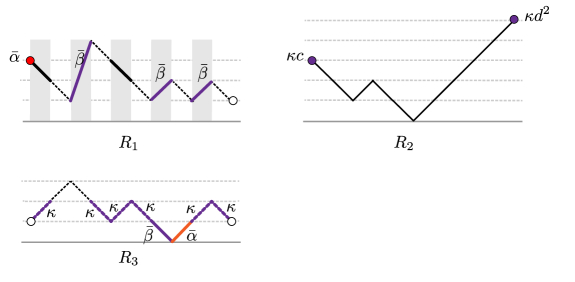
Figure 3: An example of the three types of weighted paths, $R_{1}$, $R_{2}$ and $R_{3}$.

Definition 2 ($R_{1}$ paths).

$R_{1}$ paths are lattice paths on $\Xi=\mathbb{Z}\times\mathbb{N}_{0}$ with step sets

$$\mathcal{S}_{i}(R_{1})=\left\{\begin{array}[]{ ll}\{(1,-1)\}&\text{for $i$ even (an `even down step')}\\ \{(1,2{k}-1)\,|\,{k}\in\mathbb{N}_{0}\}&\text{for $i$ odd (an `odd (jump) step').}\end{array}\right.$$ (2.17)

with $v_{0}(k)=(0,2k+1)$ for some $k\in\mathbb{N}_{0}$ and $v_{2L}=(2L,1)$. Steps in $\{(1,2{k^{\prime}}+1)\,|\,{k^{\prime}}\in\mathbb{N}_{0}\}$ are called jump up steps and the jump height is $2{k^{\prime}}+1$. The $(1,-1)$ steps are called odd down steps (if $i$ is odd) or even down steps (if $i$ is even). The weights associated with $R_{1}$ paths are

$$W^{(1)}(v_{0}(k)) =\bar{\alpha}^{k}$$ (2.18a)

$$W^{(1)}(v_{2L}) =1$$ (2.18b)

$$W^{(1)}(e_{i}) =\begin{cases}\bar{\beta}&\text{if $e_{i}=\bigl{(}(i-1,1),(i,2k^{\prime}+2)\bigr{)}$, $k^{\prime}\in\mathbb{N}_{0}$ and $i$ odd}\\ 1&\text{otherwise}\end{cases}$$ (2.18c)

Thus $R_{1}$ paths start at some odd height $y=2k+1$, every even step must be a down step, whilst an odd step may be a down step or a step up an arbitrary (odd) jump height. The path must end at $({2L},1)$. Although the $R_{1}$ paths have a step from height one to height zero, there is no step from height zero to one which combined with the constraint that the last step ends at height one means $R_{1}$ paths have no vertices with height zero. An example is shown in Figure 3.

Definition 3 ($R_{2}$ paths).

$R_{2}$ paths are lattice paths on $\Xi=\mathbb{Z}\times\mathbb{N}_{0}$ with step sets

$$\mathcal{S}_{i}(R_{2})=\{(1,-1),(1,1)\}$$ (2.19)

with $v_{0}(k)=(0,2k+1)$ for some $k\in\mathbb{N}_{0}$ and $v_{{2L}}({k^{\prime}})=(0,2{k^{\prime}}+1)$ for some ${k^{\prime}}\in\mathbb{N}_{0}$. The weights associated with $R_{2}$ paths are

$$W^{(2)}(v_{0}(k)) =\kappa\,c^{k}$$ (2.20a)

$$W^{(2)}(v_{2L}({k^{\prime}})) =\kappa\,d^{{k^{\prime}}}$$ (2.20b)

$$W^{(2)}(e_{i}) =1\qquad\text{for all $i\in[t]$}$$ (2.20c)

Thus, $R_{2}$ paths are similar to Dyck paths which start at height $2k+1$ and end at height $2{k^{\prime}}+1$ with weights on the initial and final vertices. They are also sometimes called “rigged Ballot” paths. An example is shown in Figure 3.

Definition 4 ($R_{3}$ paths).

$R_{3}$ paths are lattice paths on $\Xi=\mathbb{Z}\times\mathbb{N}_{0}$ with step set

$$\mathcal{S}_{i}(R_{3})=\{(1,-1),(1,1)\}$$ (2.21)

with initial vertex $v_{0}=(0,1)$ and final vertex $v_{2L}=(2L,1)$. The weights associated with $R_{3}$ paths are

$$W^{(3)}(v_{0}) =1,$$ (2.22a)

$$W^{(3)}(v_{2L}) =1,$$ (2.22b)

$$W^{(3)}(e_{i}) =\begin{cases}\kappa&\text{if $e_{i}=\bigl{(}(i-1,1),(i,2)\bigr{)}$ or $e_{i}=\bigl{(}(i-1,2),(i,1)\bigr{)}$}\\ \bar{\beta}&\text{if $e_{i}=\bigl{(}(i-1,1),(i,0)\bigr{)}$ }\\ \bar{\alpha}&\text{if $e_{i}=\bigl{(}(i-1,0),(i,1)\bigr{)}$ }\\ 1&\text{otherwise}\end{cases}$$ (2.22c)

Thus, $R_{3}$ are also similar to Dyck paths which start at height one and end at height one with weights on the first and second ‘levels’. An example is shown in Figure 3.

We now consider a fourth type of lattice path, which we will call $R_{4}$ or ‘canonical’ paths. They have also been called one transit paths [2] where they were used to model the behaviour of a polymer adsorbing on to an interface.

Definition 5 ($R_{4}$ paths).

$R_{4}$ paths are lattice paths on $\Xi=\mathbb{Z}\times\mathbb{N}_{0}$ with step sets

$$\mathcal{S}_{i}(R_{4})=\{(1,-1),(1,1)\}$$ (2.23)

with $v_{0}=(0,0)$, $v_{2L}=(2L,1)$ and one of the height one vertices marked. All vertices have height greater than zero. Denote the marked vertex with a dot, $\dot{v}$. If $p$ is an $R_{4}$ path and $p=v_{0}\dots\dot{v}_{k}\dots v_{2L}$, then the weights associated with $R_{4}$ paths are

$$W^{(4)}(v_{0}) =1,$$ (2.24a)

$$W^{(4)}(v_{2L}) =1$$ (2.24b)

$$W^{(4)}(e_{i}) =\begin{cases}\bar{\alpha}&\text{if $e_{i}=\bigl{(}(i-1,2),(i,1)\bigr{)}$ and $i\leq k$}\\ \bar{\beta}&\text{if $e_{i}=\bigl{(}(i-1,1),(i,2)\bigr{)}$ and $i>k$ }\\ 1&\text{otherwise}\end{cases}$$ (2.24c)

Note, $R_{4}$ paths are one-elevated, but there is a trivial bijection to zero-elevated paths, the one-elevation is merely for convenience since most of the bijections and involutions discussed in this paper result naturally with the one-elevated form. Thus $R_{4}$ paths are Dyck paths with different weights to the left and right of the marked vertex. An example is shown in Figure 4.

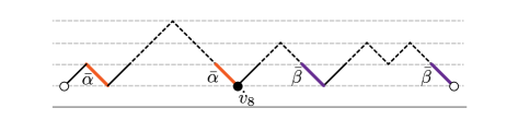
Figure 4: An example of an $R_{4}$ path.

The primary purpose of this paper is to provide a combinatorial proof of the following theorem.

Theorem 3.

Let $R_{i}(L)$ be the set of $R_{i}$ paths of length $2L$. The normalisation $Z_{L}$ defined in (2.3) for the two parameter ASEP is given by the four expressions

$$Z_{L} =\sum_{p\in R_{1}(L)}\,W^{(1)}(p)$$ (2.25a)

$$Z_{L} =\sum_{p\in R_{2}(L)}\,W^{(2)}(p)$$ (2.25b)

$$Z_{L} =\sum_{p\in R_{3}(L)}\,W^{(3)}(p)$$ (2.25c)

$$Z_{L} =\sum_{p\in R_{4}(L)}\,W^{(4)}(p)$$ (2.25d)

where $W^{(i)}(p)$ is the weight of the path $p\in R_{i}(L)$.

Remark 1.

Equations, (2.25a), (2.25b) and (2.25c) are essentially those of Theorem 2 but stated in lattice paths form. Equation (2.25d) is a new result.

As an example, for $L=2$ the four expressions obtained are

$$Z_{2}(R_{1})= \bar{\alpha}+\bar{\beta}+\bar{\alpha}\bar{\beta}+\bar{\alpha}^{2}+\bar{\beta}^{2}$$ (2.26)

$$Z_{2}(R_{2})= 5+4\kappa^{2}\frac{c}{1-cd}+4\kappa^{2}\frac{d}{1-cd}+\kappa^{2}\frac{cd}{1-cd}+\kappa^{2}\frac{c^{2}}{1-cd}+\kappa^{2}\frac{d^{2}}{1-cd}$$

$$=5+4c+4d+cd+c^{2}+d^{2}$$ (2.27)

$$Z_{2}(R_{3})= \kappa^{2}+2\bar{\alpha}\bar{\beta}\kappa^{2}+\bar{\alpha}^{2}\bar{\beta}^{2}+\kappa^{4}$$ (2.28)

$$Z_{2}(R_{4})= \bar{\alpha}+\bar{\beta}+\bar{\alpha}\bar{\beta}+\bar{\alpha}^{2}+\bar{\beta}^{2}.$$ (2.29)

We make the following remarks based on the above example.

Remark 2.

1. In equation (2.25a) the final vertex $v_{2L}=(2L,1)$ is fixed, thus, even though arbitrary high jumps steps are permitted the constraint of having to return to height one results in a finite number of contributing paths, hence the number of configurations is finite for fixed $L$, thus (2.25a) is a polynomial in $\bar{\alpha}$ and $\bar{\beta}$.

2. Equation (2.25b) is an infinite sum in $c$ and $d$, but, as will be shown, the infinite sum is always a simple geometric series giving rise to the $(1-cd)^{-1}$ factor which cancels the common factor of $\kappa^{2}=1-cd$ resulting in a polynomial in $c$ and $d$.

3. Equation (2.25c) is a polynomial in $\bar{\alpha}$, $\bar{\beta}$ and $\kappa^{2}$ arising from the three weights of the $R_{3}$ paths.

4. Equation (2.25d) is a polynomial in $\bar{\alpha}$, $\bar{\beta}$ – the same polynomial as (2.25a), but arises from a completely different set of paths.

The combinatorial proof shows how the four polynomials are connected and how the $1-cd$ factor arises in the $R_{2}$ expression – (2.25b). Combinatorially they are related by involutions and/or bijections to the fourth (2.25d). Thus there are three major parts to the proof each shows the connections between the three sets of paths and the $R_{4}$ paths.

In each of the the proofs we will need to go via several different types of path before getting to $R_{4}$ paths. Any type of path between an $R_{i}$ path and the $R_{4}$ path will be labelled $R_{i}^{j}$, being the $j^{\text{th}}$ paths on route from $R_{i}$ paths to $R_{4}$ paths.

Most of the proofs are constructed by factoring the paths into certain subpaths. We anticipate this by factoring $R_{4}$ paths into Dyck subpaths by representing the lattice path using an alphabet.

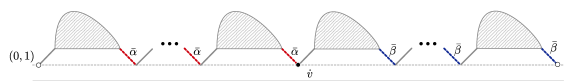
Figure 5: Schematic representation of the $D$-factorisation of a $R_{4}$ path also showing the $\bar{\alpha}$ weights to the left of all the $\bar{\beta}$ weights (which defines the marked vertex $\dot{v}$).

Denote an up step by $u$ and a down step by $d$. If we scan the word representing the path from left to right noting the step associated with each time the path returns to height one (ie. a down step from height two to height one) then we have the following classical factorisation proposition (illustrated schematically in Figure 5. ).

Proposition 2.

Let $p\in R_{4}$ with weight $\bar{\alpha}^{k}\bar{\beta}^{k^{\prime}}$, then $p$ can be written in the form

$$p=\left[\prod_{i=1}^{k}u\,D_{i}\,d\right]\left[\prod_{j=1}^{k^{\prime}}u\,D_{j+k^{\prime}}\,d\right]$$ (2.30)

where $D_{i}$ is $2$-elevated (see Definition 1) Dyck path. The weight of a $d$ step in the first factor is $\bar{\alpha}$ and the weight of a $d$ step in the second factor is $\bar{\beta}$. If either $k=0$ or ${k^{\prime}}=0$ then corresponding product is absent.

We will refer to the above factorised form as the $D$-factorisation.

2.2 Proof of Equivalence of the $R_{1}$ and $R_{4}$ path representations

We need to show

$$\sum_{p\in R_{1}}\,W^{(1)}(p)=\sum_{p\in R_{4}}\,W^{(4)}(p)\\$$ (2.31)

where the paths in the sum are all of length $2L$.

The proof is by bijection and proceeds in two stages, the first stage uses an elevated subpath factorisation to biject to $R_{1}^{1}$ paths (defined below) and the second stage bijects the $R_{1}^{1}$ paths to the $R_{4}$ paths.

When a path is represented by a step sequence (or word) the height of the initial vertex is not specified. Thus, if necessary we add the extra information by representing the path as a pair $k:w$ where $k$ is the height of the first vertex and $w$ is a word (or step sequence) in the alphabet $\{\bar{u}\,,d_{e}\,,u_{2k+1}\,\}$ where $\bar{u}\,$ is a jump down step, $d_{e}\,$ an (even) down step and $u_{2k+1}\,$ a $2k+1$, $k\geq 0$ jump step. As an example, the $R_{1}$ path illustrated in Figure 6 is represented by

$$7:u_{1}\,d_{e}\,\bar{u}\,d_{e}\,u_{3}\,d_{e}\,\bar{u}\,d_{e}\,u_{1}\,d_{e}\,\bar{u}\,d_{e}\,\bar{u}\,d_{e}\,u_{1}\,d_{e}\,u_{3}\,d_{e}\,u_{1}\,d_{e}\,\bar{u}\,d_{e}\,\,.$$ (2.32)

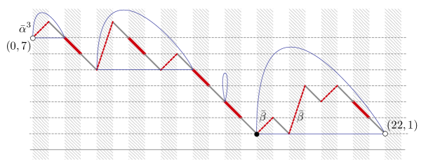
Figure 6: The 22 step $R_{1}$ path with $\bar{\alpha}$ and $\bar{\beta}$ weights given in equation (2.32) showing one level of $J$-factorisation.

We begin with a recursive factorisation of the word representing a path. The recursion is simplest to state if the path starts with the steps $d_{e}\,u_{2k+1}\,d_{e}\,$ and ends with $\bar{u}\,$, thus we define the factorisation of paths in the set

$$R^{\prime}_{1}=\{2:d_{e}\,u_{2k+1}\,d_{e}\,\,\cdot w\cdot\bar{u}\,\,|\,2k+1:w\in R_{1},\,k\geq 0\}$$ (2.33)

from which we obtain the factorisation of the paths in $R_{1}$.

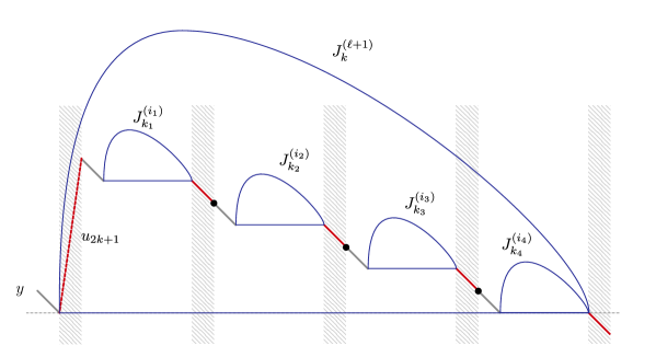
Figure 7: A schematic representation of the $J$-factorisation ($k=3$ in this case) showing one change in the level of recursion.

Stage 1: The $R^{\prime}_{1}$ paths are factorised by reading the word from left to right starting after the initial $y:d_{e}\,u_{2k+1}\,d_{e}\,$ prefix: the first time the path steps below the height $y+2k-2j+2$ defines the ‘end’ of the $J_{k_{j}}$ factor. This gives the following proposition.

Proposition 3.

Let $2k+1:w\in R_{1}$ , then $2:w^{\prime}\in R_{1}^{\prime}$, $w^{\prime}=d_{e}\,u_{2k+1}\,d_{e}\,\,\cdot w\cdot\bar{u}\,$ has the recursive factorisation,

$$w^{\prime}=d_{e}\,J_{k}^{(\ell+1)}\,\bar{u}\,= \begin{cases}d_{e}\,\bar{u}\,&\text{if $J_{k}^{(\ell+1)}=\phi$}\\ \displaystyle d_{e}\,u_{2k+1}\,\prod_{j=1}^{k+1}\left[d_{e}\,J_{k_{j}}^{(i_{j})}\bar{u}\,\right]&\text{if $J_{k}^{(\ell+1)}\neq\phi$}\end{cases}$$ (2.34)

where

$$\ell= \begin{cases}-1&\text{if $J_{k}^{(\ell+1)}=\phi$}\\ \max\{i_{j}\,|\,j=1\dots k+1\}&\text{otherwise}\end{cases}$$ (2.35)

and $J_{m}^{(n)}$ is a sub-path whose first step is a $2{m}+1$ jump step and all vertices of $J_{m}^{(n)}$ are no lower than the first vertex of the initial jump step of $J_{m}^{(n)}$. If $J_{m}^{(n)}$ is empty then the factor is denoted $J^{(0)}_{\phi}$. The superscript $n$ on $J_{m}^{(n)}$ denotes the level of recursion. The initial level is $J^{(0)}_{\phi}$.

We will refer to the above form as the $J$-factorization. The level of recursion is used primarily for induction proofs used below. One level change of factorisation is illustrated schematically in Figure 7.

For example, the path $p$, in (2.32) has the $J$-factorisation determined by factoring $d_{e}\,u_{7}\,d_{e}\,\cdot p\cdot\bar{u}\,$ using (2.34), as follows (the “$\cdot$” are only used to clarify the factorisation):

$$d_{e}\,J_{3}\,\bar{u}\, =d_{e}\,u_{7}\,d_{e}\,\cdot u_{1}\,d_{e}\,\bar{u}\,d_{e}\,u_{3}\,d_{e}\,\bar{u}\,d_{e}\,u_{1}\,d_{e}\,\bar{u}\,d_{e}\,\bar{u}\,d_{e}\,u_{1}\,d_{e}\,\bar{u}\,u_{3}\,d_{e}\,u_{1}\,d_{e}\,\bar{u}\,d_{e}\,\cdot\bar{u}\,$$

$$=d_{e}\,u_{7}\,\cdot\bigl{[}d_{e}\,u_{1}\,d_{e}\,\,\bar{u}\,\bigr{]}\cdot\bigl{[}d_{e}\,u_{3}\,\cdot\bigl{[}d_{e}\,\bar{u}\,\bigr{]}\cdot\bigl{[}d_{e}\,u_{1}\,\cdot[d_{e}\,\,\bar{u}\,]\bigr{]}\bigr{]}\cdot\bigl{[}d_{e}\,\bar{u}\,\bigr{]}\cdot$$

$$\qquad\bigl{[}d_{e}\,u_{1}\,\cdot\bigl{[}d_{e}\,u_{3}\,\cdot\bigl{[}d_{e}\,u_{1}\,\cdot[d_{e}\,\,\bar{u}\,]\bigr{]}\bigr{]}\cdot\bigl{[}d_{e}\,\bar{u}\,\bigr{]}\bigr{]}$$ (2.36)

thus, removing the prefix $$d_{e}\,u_{7}\,d_{e}\, \bar{u}\, p$$ and the suffix, gives the factorisation of as,

$$p =\bigl{[}u_{1}\,d_{e}\,\,\bar{u}\,\bigr{]}\cdot\bigl{[}d_{e}\,u_{3}\,\cdot\bigl{[}d_{e}\,\bar{u}\,\bigr{]}\cdot\bigl{[}d_{e}\,u_{1}\,\cdot[d_{e}\,\,\bar{u}\,]\bigr{]}\bigr{]}\cdot\bigl{[}d_{e}\,\bar{u}\,\bigr{]}\cdot$$

$$\qquad\bigl{[}d_{e}\,u_{1}\,\cdot\bigl{[}d_{e}\,u_{3}\,\cdot\bigl{[}d_{e}\,u_{1}\,\cdot[d_{e}\,\,\bar{u}\,]\bigr{]}\bigr{]}\cdot\bigl{[}d_{e}\,\bigr{]}\bigr{]}\,.$$ (2.37)

The ordered planar tree representation of the recursive $J$ factorisation of the path (2.32) (ie. (2.36)) is shown in Figure 8.

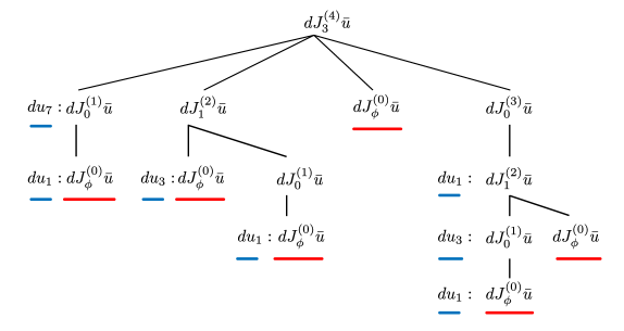
Figure 8: The ordered planar tree representation of the $J$ factorisation of the path (2.36) ($J^{(0)}_{\phi}$ is the empty factor). To read of the path the tree is traversed ‘depth-first-search with left-to-right priority’ concatenating only the ‘$du_{2k+1}$’ (underlined blue) prefixes and the ‘$dJ\bar{u}$’ factors (underlined red) on the leaves.

The only part of Proposition 3 that is not obvious is that a $J$ factor is always followed by a $\bar{u}\,$ step (ie. the first step to step below the height of a $J$ factor is always a jump down step). This can be proved inductively using the level of recursion: At level zero the most general path in $R_{1}^{\prime}$ is $d_{e}\,u_{2k+1}\,\prod_{j=1}^{k+1}\left[d_{e}\,J_{\phi}^{(0)}\bar{u}\,\right]$, thus true. If we assume the proposition is true for all paths containing level $\ell$ (or smaller) $J$ factors (illustrated schematically in Figure 7) then the number of steps in all the $J$-factors must be even since, be definition, each starts with a jump step (hence odd) and each must end on a even down step (ie. the step immediately prior to the assumed (odd) $\bar{u}\,$ step). The number of steps between two consecutive $J$-factors is two (since an odd down must followed by an even step, hence a down step). Thus the number of steps in the level $\ell+1$ $J$-factor is even. Since it starts with a (odd) jump up step and is even length, it must end with an even (down) step. Thus the next step after the $J$-factor must be an odd step and hence a jump down step. Thus if level $\ell$ is true so is level $\ell+1$ thus, by induction, true for all levels.

We now use the $J$-factorisation to biject the paths of $R_{1}$ to $R_{1}^{1}$ paths which are paths of the form

$$1:\prod_{j=1}^{k}\left[u\,J_{k_{j}}\,d\right]\,\dot{v}\,J_{k_{k+1}}\,\bar{u}\,.$$ (2.38)

All the down, $d$, steps have weight $\bar{\alpha}$ and the up, $u$, steps have unit weight. The weights of the steps in the $J_{k_{k+1}}$ factor are the same as those of the $R_{1}$ paths (ie. $\bar{\beta}$ for jump up steps from height one). The vertex $\dot{v}$ denotes the vertex which separates the $\bar{\alpha}$ weighted edges from the $\bar{\beta}$ weighted jump steps in $J_{k_{k+1}}$ and is marked. The form of the $R_{1}^{1}$ paths are shown schematically in Figure 9 (lower).

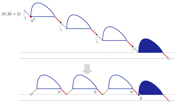
Figure 9: Schematic representation of the $\Gamma$ map defined by (2.40) whose action gives $R_{1}^{1}$ paths according to the $J$ factorisation (2.38) – here $k=3$. The blue $J$ factor contains only $\bar{\beta}$ weights.

The map $\Gamma:R_{1}\to R_{1}^{1}$, is defined as follows. If $p\in R_{1}$ and

$$d_{e}\,\,p\,\bar{u}\,=2k+2:\prod_{j=1}^{k+1}\left[d_{e}\,\,J_{k_{j}}\,\bar{u}\,\right]$$ (2.39)

then the action of $\Gamma$ is defined as

$$\Gamma(d_{e}\,\,p\,\bar{u}\,)=\begin{cases}\quad 1:\dot{v}\,p\,\bar{u}\,&\text{if $k=0$}\\ &\\ \displaystyle\quad 1:\prod_{j=1}^{k}\left[u\,J_{k_{j}}\bar{u}\,\,\right]\,\dot{v}\,J_{k_{k+1}}\bar{u}\,&\text{if $k>0$}\\ \end{cases}$$ (2.40)

The weight of each of the explicitly written $\bar{u}\,$ steps in (2.40), to the left of $\dot{v}$ (the marked vertex) is $\bar{\alpha}$. The height of the first and last vertices of the path $\Gamma(d_{e}\,\,p\,\bar{u}\,)$ are the same since $\Gamma$ has changed $k$ of the $d_{e}\,$ down steps of $d_{e}\,\,p\,\bar{u}\,$ to up steps and deleted one $d_{e}\,$ step – a height change of the first vertex of of $2k-1$. Since the first vertex of $d_{e}\,\,p\,\bar{u}\,$ was at height $2k+2$ the net change is to place the vertex at height one. This map is illustrated schematically in Figure 9 and for a particular example in Figure 10. It is straightforward to show $\Gamma$ is a bijection and so we omit the details.

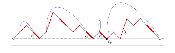
Figure 10: The result of acting with $\Gamma$ on the example in Figure 6

Stage 2: The $R_{1}^{1}$ paths have the simple factored form given by (2.40) which we now biject to $R_{4}$ paths by acting independently on each of the $J$-factors in (2.40) to produce $D$-factors. The action of the map $\Gamma^{\prime}$ on $p\in R_{1}^{1}$ is given in terms of the form (2.38) as

$$\Gamma^{\prime}(p)=\prod_{j=1}^{k}\Gamma^{\prime}\left(u\,J_{k_{j}}\,d\right)\,\dot{v}\,\Gamma^{\prime}\left(J_{k_{k+1}}\right)\,\bar{u}\,.$$ (2.41)

and the action of $\Gamma^{\prime}$ on a $u\,J_{k}\,d$ factor is defined recursively using the factorisation (2.34) (omitting the level superscripts) by

$$\Gamma^{\prime}\left(d_{e}\,J_{k}\,\bar{u}\,\right)=\begin{cases}\displaystyle d\,&\text{if $J_{k}=\phi$}\\ \displaystyle d\,u\,\cdot u\,^{k}\prod_{j=1}^{k+1}\Gamma^{\prime}\left(d_{e}\,J_{k_{j}}\bar{u}\,\right)&\text{if $J_{k}\neq\phi$}\end{cases}$$ (2.42)

Thus $\Gamma^{\prime}$ has replaced the first $d_{e}\,$ of (2.34) (of the righthand side case two) by $d$ and the $u_{2k+1}$ step by $u^{k+1}$. Any $\bar{\alpha}$ weighted $d$ step retains the $\bar{\alpha}$ weight under the action of $\Gamma^{\prime}$. All the $\bar{\beta}$ weights are associated with the jump up steps (from height one – see Figure 6) in the rightmost $J$-factor ie. $J_{k_{k+1}}$ and under $\Gamma^{\prime}$ the $\bar{\beta}$ weight is associated with the leftmost $u$ step of (2.42).

We define $D$ by

$$d\,D=\Gamma^{\prime}\left(d_{e}\,J_{k}\,\bar{u}\,\right).$$ (2.43)

where the use of $D$ signifies that $\Gamma^{\prime}$ produces elevated Dyck subpaths (proved below).

The $\Gamma^{\prime}$ map is illustrated schematically in Figure 11.

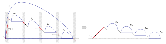
Figure 11: Schematic representation of the $\Gamma^{\prime}$ map defined by (2.42) – (here $k=3$) giving a Dyck path.

For example, with $\Gamma^{\prime}$ applied to (2.32) via the factorisation (2.44) the image path is:

$$\Gamma^{\prime}(d_{e}\,J_{3}\,\bar{u}\,) =d\,u\,^{4}\cdot\Gamma^{\prime}(d_{e}\,J_{0}\,\bar{u}\,)\cdot\Gamma^{\prime}(d_{e}\,J_{1}\,\bar{u}\,)\cdot\Gamma^{\prime}(d_{e}\,\bar{u}\,)\cdot\Gamma^{\prime}(d_{e}\,J_{0}\,\bar{u}\,)$$

$$=d\,u\,^{4}\cdot[d\,u\,^{1}\cdot\Gamma^{\prime}(d_{e}\,\bar{u}\,)]\cdot[d\,u\,^{2}\cdot\Gamma^{\prime}(d_{e}\,\bar{u}\,)\cdot\Gamma^{\prime}(d_{e}\,J_{0}\,\bar{u}\,)]\cdot d\,\cdot\dot{v}_{3}\cdot[d\,u\,^{1}\cdot\Gamma^{\prime}(d_{e}\,J_{1}\,\bar{u}\,)\bigr{]})]$$

$$=d\,u\,^{4}\cdot[d\,u\,^{1}\cdot d\,]\cdot[d\,u\,^{2}\cdot d\,]\cdot[d\,u\,^{1}\cdot\Gamma^{\prime}(d_{e}\,\bar{u}\,)]\cdot d\,\cdot$$

$$\qquad[d\,u\,^{1}\cdot d\,u\,^{2}\cdot\Gamma^{\prime}(d_{e}\,J_{0}\,\bar{u}\,)\cdot\Gamma^{\prime}(d_{e}\,\bar{u}\,)]$$

$$=d\,u\,^{4}\cdot[d\,u\,^{1}\cdot d\,]\cdot[d\,u\,^{2}\cdot d\,]\cdot[d\,u\,^{1}\cdot d\,]\cdot d\,\cdot$$

$$\qquad[d\,u\,^{1}\cdot d\,u\,^{2}\cdot d\,u\,^{1}\cdot\Gamma^{\prime}(d_{e}\,\bar{u}\,)\cdot[d\,]]$$

$$=d\,u\,^{4}\cdot[d\,u\,^{1}\cdot d\,]\cdot[d\,u\,^{2}\cdot d\,]\cdot[d\,u\,^{1}\cdot d\,]\cdot d\,\cdot$$

$$\qquad[d\,u\,^{1}\cdot d\,u\,^{2}\cdot d\,u\,^{1}\cdot[d\,]\cdot[d\,]]$$

$$=d\,u\,^{4}d\,u\,^{1}d\,d\,u\,^{2}d\,d\,u\,^{1}d\,d\,\cdot d\,u\,^{1}d\,u\,^{2}d\,u\,^{1}d\,d\,$$ (2.44)

The result of acting with $\Gamma^{\prime}$ on the example in Figure 10 is shown in figure Figure 12.

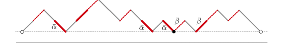
Figure 12: The result of acting with $\Gamma^{\prime}$ on the example in Figure 9

The path configurations after acting with $\Gamma^{\prime}$ is that of $R_{4}$ except for that the $\bar{\beta}$ weights are on the up step (from height one to two) rather than on the down step (form height two to one) however this is readily fixed just by moving the weight across.

We now prove by induction on the level of recursion that the $D$ factor of (2.43) is an elevated Dyck path. Clearly the step set of $D$ is that of Dyck paths. What needs justification is that that paths in $D$ start and end at the same height and no vertices of the path are below that of the initial vertex.

Re-instating the level of recursion with a superscript and subscripts to distinguish the $D$ factors, the initial step of the induction corresponds to with $J^{(0)}_{k}=\phi$ in which case $d\,D^{(0)}_{k}=\Gamma\left(d_{e}\,\bar{u}\,\right)=d$, thus $D^{(0)}_{k}=\phi$ which is an (empty) Dyck path. Inducting from level $\ell$ to $\ell+1$ we have

$$d\,D^{(\ell+1)}_{k}=\Gamma^{\prime}\left(d_{e}\,J^{(\ell+1)}_{k}\,\bar{u}\,\right) =d\,u\,^{k+1}\prod_{j=1}^{k+1}\Gamma^{\prime}\left(d_{e}\,J^{(i_{j})}_{k_{j}}\bar{u}\,\right)$$ (2.45)

$$=d\,u\,^{k+1}\prod_{j=1}^{k+1}\left[d\,D^{(i_{j})}_{k_{j}}\right]$$ (2.46)

where, as in (2.35), $$\ell=\max\{i_{j}\,|\,j=1...k+1\}$$, thus

$$D^{(\ell+1)}_{k} =u\,^{k+1}\prod_{j=1}^{k+1}\left[d\,D^{(i_{j})}_{k_{j}}\right].$$ (2.47)

If we assume for all levels $i_{j}\leq\ell$ each $D^{(i_{j})}_{\ell}$ is an elevated Dyck path (and hence the first and last vertices are the same height) and since the prefix $u\,^{k+1}$ in (2.47), goes up $k$ steps and the product steps down $k+1$ times (ie. the $k+1$, $d$ steps), the righthand side is also a Dyck path, that is $D^{(\ell+1)}_{k}$ is a Dyck path, thus by induction the proposition is true.

2.3 Proof of Equivalence of the $R_{2}$ and $R_{4}$ path representations

We prove this equivalence in four stages. The four stages are connected by either a bijection or a sign reversing involution. The five intermediate sets of paths involved, $R_{2}^{i}$, $i=1..5$ are defined when each stage is discussed in detail below.

• $R_{2}\,\xrightarrow{\,\kappa^{2}\,}\,R_{2}^{1}\,\xrightarrow{\,\Phi_{2}^{12}\,}\,R_{2}^{2}$. A sign reversing involution, $\Phi_{2}^{12}$, which reduces the infinite sum (2.25b) over $R_{2}$ paths to a finite sum over $R_{2}^{2}$ paths. The involution acts on an enlarged path set $R_{2}^{1}$, obtained from $R_{2}$ paths by expanding $\kappa^{2}=1-cd$. The fixed point set of $\Phi^{12}_{2}$ is the set of $R_{2}^{2}$ paths.

• $R_{2}^{2}\,\xrightarrow{\,\Gamma_{2}^{23}\,}\,R_{2}^{3}$. The bijection $\Gamma_{2}^{23}$ ‘pulls down’ the first and last vertices of each path thus replacing the sum over $R_{2}^{2}$ paths by a sum over $R_{2}^{3}$ paths (which start and end at height one).

• $R_{2}^{3}\,\xrightarrow{\,\Gamma_{2}^{34}\,}\,R_{2}^{4}$. The bijection $\Gamma_{2}^{34}$ ‘lifts’ the $R_{2}^{3}$ paths above the surface to give $R_{2}^{4}$ paths (which have no height zero vertices).

• $R_{2}^{4}\,\xrightarrow{\,c,d\to\bar{\alpha},\bar{\beta}}\,R_{2}^{5}\,\xrightarrow{\,\Phi_{2}^{56}\,}\,R_{4}$. The final sign reversing involution, $\Phi_{2}^{56}$, replaces the $c$ and $d$ weighted paths of $R_{2}^{4}$ with $\bar{\alpha}$ and $\bar{\beta}$ weighted paths. The involution acts on an enlarged set of paths, $R_{2}^{5}$, obtained by expanding $c=1-\bar{\alpha}$ and $d=1-\bar{\beta}$. The fixed point set is the path set $R_{4}$.

In summary,

$$R_{2}\,\xrightarrow{\,\kappa^{2}\to 1-cd\,}\,R_{2}^{1}\,\xrightarrow{\,\Phi_{2}^{12}\,}\,R_{2}^{2}\,\xrightarrow{\,\Gamma_{2}^{23}\,}\,R_{2}^{3}\,\xrightarrow{\,\Gamma_{2}^{34}\,}\,R_{2}^{4}\,\xrightarrow{\,c,d\to\bar{\alpha},\bar{\beta}}\,R_{2}^{5}\,\xrightarrow{\,\Phi_{2}^{56}\,}\,R_{4}$$ (2.48)

We now expand on each of the four stages.

Stage 1.

$R_{2}\,\xrightarrow{\,\kappa^{2}\,}\,R_{2}^{1}\,\xrightarrow{\,\Phi_{2}^{12}\,}\,R_{2}^{2}$. The sign reversing involution is defined on the set of paths $R_{2}^{1}$ which is constructed by using $\kappa^{2}=1-cd$ to enlarge the size of the weighted set $R_{2}$ (which has weights given by (2.20)). Thus for each weighted path $\omega\in R_{2}$ (which always has a factor of $\kappa^{2}$ in its weight) we replace by two paths $\omega_{1}$ and $\omega_{2}$, where $\omega_{1}$ is the same sequence of steps as $\omega$, but the initial and final vertex weights are $w^{i}((0,2k+1))=c^{k}$ and $w^{f}((2L,2k^{\prime}+1))=d^{k^{\prime}}$ (ie. no factors of $\kappa$). Similarly, $\omega_{2}$ is the same sequence of steps as $\omega$, but the initial and final vertex weights are $w^{i}((0,2k+1))=-c^{k+1}$ and $w^{f}((2L,2k^{\prime}+1))=d^{k^{\prime}+1}$ ie. each vertex has an extra factor of $c$ (or $d$), and an overall negative weight). Thus we have that

$$Z_{2L}^{(2)} =\sum_{\omega\in R_{2}^{1}}W^{(2)}_{2}(\omega)$$ (2.49)

where the weight $W^{(2)}_{2}$ is as just explained. The $R_{2}^{2}$ paths are a subset of the $R_{2}$ paths, given by

$$R_{2}^{2}=\{p\in R_{2}\,|\,\text{$p$ has at least one vertex of height one}\}$$ (2.50)

We will now show that $R_{2}^{2}$ is the fixed point set of $R_{2}^{1}$ under the sign reversing involution $\Phi_{2}^{12}$ defined below. The signed set $\Omega^{(2)}=R_{2}^{1}=\Omega^{(2)}_{+}\cup\Omega^{(2)}_{-}$ is defined by:

$$\Omega^{(2)}_{+} =\{\omega\,|\,\text{$\omega\in R_{2}^{2}$ and $W^{(1)}_{2}(\omega)>0$}\}$$ (2.51)

$$\Omega^{(2)}_{-} =\{\omega\,|\,\text{$\omega\in R_{2}^{2}$ and $W^{(1)}_{2}(\omega)<0$}\}.$$ (2.52)

The involution $\Phi_{2}^{12}\,:\,\Omega^{(2)}\to\Omega^{(2)}$ is defined by three cases. Let $\omega\in\Omega^{(2)}$, $\omega^{\prime}=\Phi_{2}^{12}(\omega)$ and let $v_{0}$ be the first vertex of $\omega$ and $v_{2L}$ the last. Recall, $w(v)$ is the weight of vertex $v$.

• (Negative weight.) If $v_{0}=(0,2k+1)$, $v_{2L}=(2L,2k^{\prime}+1)$, $k,k^{\prime}\geq 0$ and $w^{i}(v_{0})=-c^{k+1}$ then $\omega^{\prime}$ is a path with the same sequence of steps as $\omega$, but initial vertex $v_{0}^{\prime}=(0,2k+3)$, final vertex $v_{2L}=(2L,2k^{\prime}+3)$ (ie. is $\omega$ ‘pushed up’ two units), and has vertex weights $w(v^{\prime}_{0})=c^{k+1}$ and $w(v^{\prime}_{2L})=d^{k+1}$. For any $\omega$, $\omega^{\prime}$ always exists and has opposite sign to $\omega$, thus $\Phi_{2}^{12}$ is sign reversing for this case.

• (Positive weight, no height one vertices.) If $v_{0}=(0,2k+1)$, $v_{2L}=(2L,2k^{\prime}+1)$, $k,k^{\prime}\geq 1$, $w(v_{0})=c^{k}$ and $\omega$ has no vertex with height one, then $\omega^{\prime}$ is a path with the same sequence of steps as $\omega$, but initial vertex $v_{0}^{\prime}=(0,2k-1)$, final vertex $v_{2L}=(2L,2k^{\prime}-1)$ (ie. is $\omega$ “pushed down” two units), and has vertex weights $w(v^{\prime}_{0})=c^{k}$ and $w(v^{\prime}_{2L})=d^{k}$. Since $\omega$ no height one vertices, all its vertices have height greater than two, thus when $\omega$ is pushed down no vertices have height less than zero and hence $\omega^{\prime}\in\Omega^{(2)}$. For any $\omega$ in this case, $\omega^{\prime}$ always exists and has opposite sign to $\omega$, thus $\Phi_{2}^{12}$ is sign reversing for this case.

• (Positive weight, at least one height one vertex.) If $\omega$ has positive weight and at least one vertex with height one, then $\omega^{\prime}=\omega$.

Clearly, if $\omega$ corresponds to Case 1, then $\omega^{\prime}$ is a unique path corresponding to Case 2 and visa versa. Case 3 is the fixed point set. Since the fixed point set paths are in the positive set, $\Omega_{+}^{(2)}$, they have weight $c^{k}$ for the initial, height $2k+1$ vertex and weight $d^{k^{\prime}}$ for the last, height $2k^{\prime}+1$ vertex. Thus $\Phi_{2}^{12}$ is a sign reversing involution with fixed point set the subset of $R_{2}^{1}$ paths with at least one vertex at height one and positive weight ie. $R_{2}^{2}$ paths.

The paths in $R_{2}^{3}$ have at least one vertex with height one and may have many with height zero. We ‘biject away’ the latter subset in the next stage.

Stage 2.

$R_{2}^{2}\,\xrightarrow{\,\Gamma_{2}^{23}\,}\,R_{2}^{3}\,$. We now map the path set to a subset $R_{2}^{3}$ of $R_{2}^{2}$ paths which do not intersect the line $y=0$. In order to do this the resulting paths have to carry a “dividing” line (or equivalently a marked vertex). Thus, if

$$\hat{R}_{2}^{2} =\{p\in R_{2}^{2}\,|\,\text{$p$ has no height zero vertices}\}$$ (2.53)

then

$${R}_{2}^{3} =\ \text{set of paths of $\hat{R}_{2}^{2}$ with one height one vertex marked.}$$ (2.54)

That is, if $p\in{R}_{2}^{3}$ has $m$ vertices with height one, then $p$ produces $m$ paths in ${R}_{2}^{3}$ each one with one of the $m$ vertices marked.

Let $p\in R_{2}^{2}$. If $p$ starts at height $2k+1$ and ends at height $2\ell+1$ then, using a similar factorisation to the $D$-factorisation of the $R_{1}$ to $R_{4}$ bijection – Lemma 2, $p$ can be factorised as

$$\left[\prod_{n=1}^{2k}D_{n}d\right]B\left[\prod_{m=1}^{2\ell}uD^{\prime}_{m}\right]$$ (2.55)

where $D_{n}$ and $D^{\prime}_{m}$ are (possibly empty ) elevated Dyck paths, $u$ an up step, $d$ a down step and $B$ is defined by the fact that $uBd$ is a Dyck path.

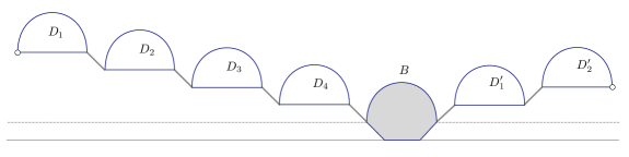
Figure 13: An schematic representation of the factorisation (2.55) (here $k=2$, $\ell=1$).

That is, $B$ is the subpath of $p$ which is made of only up and down steps and whose first vertex is the leftmost height one vertex of $p$ and whose last vertex is the rightmost height one vertex of $p$. If $k$ or $\ell$ is zero then the respective product is absent. The factorisation is shown schematically in Figure 13.

We now construct a map, $\Gamma_{2}^{23}:R_{2}^{2}\to R_{2}^{3}$, that eliminates all steps of the subpath $B$, below $y=1$ and replaces it with a path, $\hat{B_{L}}|\hat{B_{R}}$, which has no height zero vertices but has a ‘dividing line’ (or marked vertex) – see Figure 14.

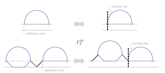
Figure 14: An schematic representation of the action of the bijection $\Gamma_{2}^{23}$ on the $B$ factor at stage 2. Case with no step below $y=1$ (upper) and the case with at least one step below $y=1$ (lower).

The map $\Gamma_{2}^{23}$ acts on $B$ as follows. If $B$ has no steps below $y=1$, then $B^{\prime}=\Gamma_{2}^{23}(B)=|B$, where $|$ denotes a vertical dividing line drawn through the leftmost vertex of $B$. If $B$ has at least one step below $y=1$, then let $u^{\prime}$ be the rightmost (up) step from $y=0$ to $y=1$. Thus $B$ factorises as $B=w_{1}u^{\prime}w_{2}$, and then $B^{\prime}=u^{\prime}w_{1}|w_{2}$, where $|$ denotes a vertical dividing line drawn through the vertex between $w_{1}$ and $w_{2}$. Note, since $u^{\prime}$ is an up step, none of the steps of the subpath $u^{\prime}w_{1}$ intersect $y=0$. Thus $B^{\prime}$ does not intersect $y=0$. The map $\Gamma_{2}^{23}$ acting on all factors of the form of $B$ is readily seen to be injective and surjective and thus a bijection (the dividing line shows where the first up step has to be moved under the action of the inverse map $\left(\Gamma_{2}^{23}\right)^{-1}$).

The action of $\Gamma_{2}^{23}$ on $p\in R_{2}^{2}$ only depends on its $B$ factor and is defined as

$$\Gamma_{2}^{23}(p)=\Gamma_{2}^{23}\left(\prod_{n=1}^{2k}D_{n}d\cdot B\cdot\prod_{m=1}^{2\ell}uD^{\prime}_{m}\right)=\prod_{n=1}^{2k}D_{n}d\cdot\Gamma_{2}^{23}(B)\cdot\prod_{m=1}^{2\ell}uD^{\prime}_{m}$$ (2.56)

with the weight of all vertices unchanged. Thus the path $\Gamma_{2}^{23}(p)$ has the same weight as $p$, does not intersect $y=0$ and has a dividing line, that is, $\Gamma_{2}^{23}(p)\in R_{2}^{3}$.

Stage 3.

$R_{2}^{3}\,\xrightarrow{\,\Gamma_{2}^{34}\,}\,R_{2}^{4}$. The map $\Gamma_{2}^{34}$ ‘rotates down’ the initial and final vertices of the path to produce a path which starts and ends at $y=1$, but has a subset of “marked” $c$ and $d$ height one vertices. This is a simple extension of the same map given in [3] and hence we only discuss it briefly here. It is illustrated schematically in Figure 15.

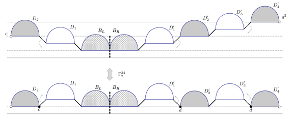
Figure 15: An schematic representation of the bijection $\Gamma_{2}^{34}$ of stage 3.

Let $p\in R_{2}^{3}$ start at $y=2k+1$, and end at $2\ell+1$, (and hence has weight $c^{k}d^{\ell}$). Using the factorisation (2.56),

$$p=\prod_{n=1}^{2k}D_{2k-n+1}d\cdot B_{L}|B_{R}\cdot\prod_{m=1}^{2\ell}uD^{\prime}_{m}$$ (2.57)

we can define $\Gamma_{2}^{34}$ by

$$\Gamma_{2}^{34}(p)=\left(\prod_{n=1}^{k}D_{2k-2n+2}\cdot\dot{v}(c)\cdot u\,D_{2k-2n+1}d\right)\cdot B_{L}|B_{R}\cdot\left(\prod_{m=1}^{\ell}u\,D^{\prime}_{2m-1}d\cdot\dot{v}(d)\cdot D^{\prime}_{2m}\right)$$ (2.58)

where, $\dot{v}(c)$ and $\dot{v}(d)$ represent a marked vertex between the two steps where it occurs (and is weighted $c$ and $d$ respectively) – see Figure 15. Each mark to the left of the dividing line carries weight $c$ and each of those to the right of $|$ carry a weight $d$. The inverse map $\left(\Gamma_{2}^{34}\right)^{-1}$ uses the marked vertices to fix the step change $u\to d$.

Stage 4.

$R_{2}^{4}\,\xrightarrow{\,c,d\to\bar{\alpha},\bar{\beta}}\,R_{2}^{5}\,\xrightarrow{\,\Phi_{2}^{56}\,}\,R_{4}$. In the final stage we define an involution, $\Phi_{2}^{56}$ whose fixed point set is $R_{4}$ with weights $\bar{\alpha}$ and $\bar{\beta}$. Starting with the set of all paths given at Stage 3, ie. of the form(2.58), we construct a larger set of paths, $R_{2}^{5}$, using the same construction of Stage 1, that is, by replacing all weights $c$ with $\bar{\alpha}-1$ and all weights $d$ by $\bar{\beta}-1$. Thus each path in $R_{2}^{4}$, which has weight $c^{k}d^{\ell}$, maps to $2^{k+\ell}$ paths. Combinatorially, this set has all marked vertices, $\dot{v}(c)$ (ie. to the left of $|$), replaced by either a weight of $-1$ or $\bar{\alpha}$ and all marked vertices, $\dot{v}(d)$ (ie. to the right of $|$), replaced by either a weight of $-1$ or $\bar{\beta}$. All remaining vertices of the path intersecting $y=1$, except that intersecting the dividing line, will be labeled with ‘$+1$’. The weight of a given path is a product of all the $\bar{\alpha}$, $\bar{\beta}$ and $-1$ factors. Thus the weight of the path will be negative if there are an odd number of factors of $-1$.

This construction defines the elements of the set $\Omega=\Omega_{+}\cup\Omega_{-}$ where $\Omega_{+}$ contains the positive weighted paths and $\Omega_{-}$ the negative weighted paths.

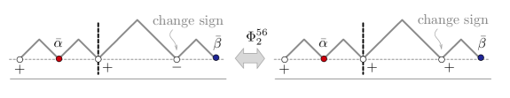
Figure 16: An example of a cancelling a pair of partially marked paths – the rightmost $\pm 1$ weighted vertex is changed to a $\mp 1$ weight.

The involution, $\Phi_{2}^{56}$, is straightforward: If $p\in\Omega$ has no $+1$ or $-1$ vertices then $p^{\prime}=\Phi_{2}^{56}(p)=p$. All these cases obviously have positive weight with all height one vertices to the left of the dividing line carrying weight $\bar{\alpha}$ and those to the right, weight $\bar{\beta}$. These are the fixed point paths and are clearly $R_{4}$ paths (after deleting the dividing line – which is no longer necessary). If $p\in\Omega$ has at least one $+1$ or $-1$ vertex then $p^{\prime}=\Phi_{2}^{56}(p)$ is the same weighted path as $p$ except the rightmost signed vertex has opposite sign (and hence $p^{\prime}$ has the same weight as $p$ except of opposite sign) – see Figure 16. Clearly, $\left(\Phi_{2}^{56}\right)^{2}=1$.

2.4 Proof of Equivalence of the $R_{3}$ and $R_{4}$ path representations

We prove the equivalence using a sign reversing involution, $\Phi_{3}$. The fixed point set will be the set of paths $R_{4}$. Before defining the signed set of the involution we re-weight the steps of the $R_{3}$ paths as follows. The paths in $R_{3}$ have steps from height two to one and height one to two each weighted by $\kappa$ (see Definition 3). Since all the paths in $R_{3}$ start and end at height one, all paths have an even number of steps between heights two and one and thus each path has an even degree $\kappa$ weight ie. $\kappa^{2k}$ (readily proved by induction on the length of the path). Thus rather than have $\kappa$ weights associated with up and down steps we associate a $\kappa^{2}$ weight only with a down step (from height two to one). Similarly there are an even number of steps between heights zero and one. These carry weights $\bar{\alpha}$ and $\bar{\beta}$ so we collect the two weights together to form a single $\bar{\alpha}\bar{\beta}$ weight associated with the up step from height zero to one and give the down step unit weight. Call this reweighed path set, $R_{3}^{\prime}$. An example is shown in Figure 17 (which is a re-weighting of the example in Figure 3).

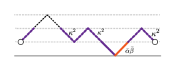
Figure 17: An example of a re-weighted $R_{3}$ path.

We now increase the size of $R_{3}^{\prime}$ by expanding all $\kappa^{2}=\bar{\alpha}+\bar{\beta}-\bar{\alpha}\bar{\beta}$ weights. Thus any path, $\omega$ with an edge, $e_{n}$ with weight $\kappa^{2}$ gives rise to three paths, $\omega_{1}$, $\omega_{2}$ and $\omega_{3}$, with the same step sequence, but different weights: $\omega_{1}$ is the same path as $\omega$, but edge $e_{n}$ has weight $\bar{\alpha}$. Similarly, for $\omega_{2}$, edge $e_{n}$ has weight $\bar{\beta}$ and for $\omega_{3}$, edge $e_{n}$ has negative weight $-\bar{\alpha}\bar{\beta}$. Thus if the path has a weight factor $\kappa^{2k}$ it will give rise to $3^{k}$ paths. Call this expanded set, $R_{3}^{2}$. Note, all the $-\bar{\alpha}\bar{\beta}$ weights are between heights two and one whilst all the $\bar{\alpha}\bar{\beta}$ weights are between heights zero and one.

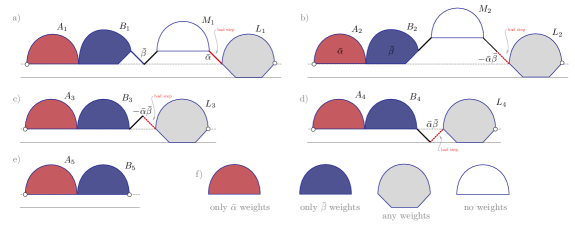
Figure 18: a) – e) Schematic representations of the five possible factorisations of $R_{3}$ paths as defined by the position of the ‘bad’ step – see (2.59). f) Key for weight structure of subpath factors.

The involution depends on the following factorisation of the paths in $R_{2}^{2}$.

Lemma 1.

Let $\omega\in R_{2}^{2}$, then $\omega$ can be factorised in one and only one of the five following forms (illustrated in Figure 18):

$$\omega^{(1)} =A_{1}B_{1}\,duM_{1}\,d^{\prime}\,L_{1} w(d)=\bar{\beta},\quad w(d^{\prime})=\bar{\alpha}$$ (2.59a)

$$\omega^{(2)} =A_{2}B_{2}\,uM_{2}dd^{\prime}\,L_{2}\, w(d^{\prime})=-\bar{\alpha}\bar{\beta}$$ (2.59b)

$$\omega^{(3)} =A_{3}B_{3}\,u\,d\,L_{3}, w(d)=-\bar{\alpha}\bar{\beta}$$ (2.59c)

$$\omega^{(4)} =\,A_{4}B_{4}du\,L_{4}, w(u)=\bar{\alpha}\bar{\beta}$$ (2.59d)

$$\omega^{(5)} =\,A_{5}B_{5}$$ (2.59e)

where $$u u^{\prime} d d^{\prime} A_{i} B_{i}d M_{i} uL_{i}d w(e_{n}) e_{n} A_{i} \bar{\alpha} B_{i} \bar{\beta} M_{i} L_{i} \bar{\alpha} \bar{\beta} \bar{\alpha}\bar{\beta} -\bar{\alpha}\bar{\beta}$$, are up steps, , are down steps, , , and are all (possibly empty) elevated Dyck subpaths and is the weight of step . The subpaths contain only weighted steps, the subpaths contain only weighted steps, the subpaths contain no weighted steps and the subpaths contain any weighted steps (ie. , , and ).

The factorisation is defined by what will be referred to as a “bad” step. Bad steps (if they occur) are of two types: 1) an ‘$\bar{\alpha}\bar{\beta}$-bad’ step or 2) an ‘$\bar{\alpha}$-bad’ step. An $\bar{\alpha}\bar{\beta}$-bad step is the leftmost step weighted $\pm\bar{\alpha}\bar{\beta}$ and an $\bar{\alpha}$-bad step is the leftmost step weighted $\bar{\alpha}$ occurring to the right of a step weighted $\bar{\beta}$. Note, the $R_{4}$ paths are precisely the paths with no bad steps. The factorisation cases are as follows:

• The path has a bad step:

  • The leftmost bad step is an $\bar{\alpha}$-step. Thus to the left of the $\bar{\alpha}$-step there are no $\bar{\alpha}\bar{\beta}$ weighted steps and hence the path must factor according to case (2.59a).

  • The leftmost bad step is an $\bar{\alpha}\bar{\beta}$-step. There are two sub-cases:

    • The $\bar{\alpha}\bar{\beta}$-step is above height one (ie. negative). We split this into two further cases depending on:

      • whether the step before the bad step is a down step – case (2.59b)

      • or an up step – case (2.59c).

    • The $\bar{\alpha}\bar{\beta}$-step is below height one (ie. positive). This is case (2.59d).

• The path has no bad step – thus contains no $\bar{\alpha}\bar{\beta}$ steps and all the $\bar{\alpha}$ steps are to the left of the $\bar{\beta}$ steps. This is case (2.59e).

The involution $\Phi_{3}$, detailed below, can be succinctly summarised as follows. Referring to Figure 18: In (a) flip the pair of edges to the left of $M_{1}$, one of which is now a down edge and move this one to the other side of $M_{1}$ together with the factor $\bar{\beta}$ (and change its sign). This is now the same as (b). In (c) flip the pair of edges to the left of $M_{1}$ and change the sign giving and (d). Hence (a) and (b) cancel as do (c) and (d) leaving only (e).

The involution $\Phi_{3}$ is defined on the path set $R_{3}^{2}$ and will have fixed point set $R_{4}$. Define the signed set as follows. Let

$$R_{3}^{2} =\Omega^{(3)}_{+}\cup\Omega^{(3)}_{-}$$ (2.60)

where the signed sets are

$$\Omega^{(3)}_{+} =\{\omega\,|\,\text{$\omega\in R_{2}^{2}$ and $\omega$ has positive weight}\}$$ (2.61)

$$\Omega^{(3)}_{-} =\{\omega\,|\,\text{$\omega\in R_{2}^{2}$ and and $\omega$ has negative weight}\}.$$ (2.62)

The involution $\Phi_{3}:R_{3}^{2}\to R_{3}^{2}$, falls into five cases corresponding to the five factorisations. Let $\omega\in R_{3}^{2}$ and $\omega^{\prime}=\Phi_{3}(\omega)$.

1. If $\omega$ is of the form of (2.59a) then $\omega^{\prime}$ is obtained from $\omega$ by moving $d$ to the right of $d^{\prime}$, removing the $\bar{\alpha}$ and $\bar{\beta}$ weights from $d$ and $d^{\prime}$ and giving the moved $d$ step weight $-\bar{\alpha}\bar{\beta}$, that is,

   $$A_{1}B_{1}\,duM_{1}\,d^{\prime}\,L_{1}\longrightarrow\omega^{\prime}=A_{1}B_{1}\,uM_{1}d^{\prime}d\,L_{1}$$ (2.63)

   Thus $\omega^{\prime}$ is of the form and weight of (2.59b). In $\omega^{\prime}$, $w(d)w(d^{\prime})=-\bar{\alpha}\bar{\beta}$ and thus the sign of $\omega^{\prime}$ is opposite to that of $\omega$ as required.

2. If $\omega$ is of the form of (2.59b) then $\omega^{\prime}$ is obtained from $\omega$ by shifting $d$ to the left of $u$, changing the weight of $d$ to $\bar{\beta}$, and that of $d^{\prime}$ to $\bar{\alpha}$, to give

   $$A_{2}B_{2}\,uM_{2}dd^{\prime}\,L_{2}\to\omega^{\prime}=A_{2}B_{2}\,duM_{2}\,d^{\prime}\,L_{2}$$ (2.64)

   Thus $\omega^{\prime}$ is of the form and weight of (2.59a). Since now $w(d)w(d^{\prime})=+\bar{\alpha}\bar{\beta}$ the sign of $\omega^{\prime}$ is opposite to that of $\omega$ as required.

3. If $\omega$ is of the form of (2.59c) then $\omega^{\prime}$ is obtained from $\omega$ by swapping the $u$ and $d$ steps and changing the weight of $d$ to $+\bar{\alpha}\bar{\beta}$, to give

   $$A_{3}B_{3}\,u\,d\,L_{3}\longrightarrow\omega^{\prime}=A_{3}B_{3}\,d\,u\,L_{3}$$ (2.65)

   Thus $\omega^{\prime}$ is of the form (2.59d). Since now $w(d)=+\bar{\alpha}\bar{\beta}$ the sign of $\omega^{\prime}$ is opposite to that of $\omega$ as required.

4. If $\omega$ is of the form of (2.59d) then $\omega^{\prime}$ is obtained from $\omega$ by swapping the $u$ and $d$ steps and changing the weight of $d$ to $-\bar{\alpha}\bar{\beta}$ to give

   $$A_{4}B_{4}\,d\,u\,L_{4}\longrightarrow\omega^{\prime}=A_{4}B_{4}\,u\,d\,L_{4}$$ (2.66)

   Thus $\omega^{\prime}$ is of the form (2.59c). Since now $w(d)=-\bar{\alpha}\bar{\beta}$ the sign of $\omega^{\prime}$ is opposite to that of $\omega$ as required.

5. If $\omega$ is of the form of (2.59) then $\omega^{\prime}=\omega$. This is the fixed point set.

In all cases after the action of $\Phi_{3}$, the bad step stays immediately to the left of the initial $L_{i}$ factor thus ensuring $\Phi_{3}^{2}=1$ as required. The fixed point set has no bad steps ie. all the $\bar{\alpha}$ weighted steps are to the left of the $\bar{\beta}$ steps and there are no $\pm\bar{\alpha}\bar{\beta}$ weighted steps – thus the fixed point set is the set $R_{4}$ as desired.

References

- [1] R. A. Blythe and M. R. Evans. Topical Review: Nonequilibrium steady states of matrix-product form: a solver’s guide. Journal of Physics A Mathematical General, 40:333, November 2007.
- [2] R Brak, J de Gier, and V Rittenberg. Nonequilibrium stationary states and equilibrium models with long range interactions. J. Phys. A: Math. Gen., 37:4303–4320, 2004.
- [3] R Brak and J W Essam. Return polynomials for non-intersecting paths above a surface on the directed square lattice. J. Phys. A: Math. Gen., 34:10763–10782, 2001.
- [4] R Brak and J W Essam. Asymmetric exclusion model and weighted lattice path. J. Phys. A: Math. Gen., 37:4183–4217, 2004.
- [5] S. Corteel, R. Brak, A. Rechnitzer, and J. Essam. A combinatorial derivation of the pasep alegebra. In FPSAC 2005. Formal Power Series and Algebraic Combinatorics, 2005.
- [6] B Derrida, M Evans, V Hakin, and V Pasquier. Exact solution of a 1d asymmetric exclusion model using a matrix formulation. J. Phys. A: Math. Gen., 26:1493 – 1517, 1993.
- [7] E Duchi and G Schaeffer. A combinatorial approach to jumping particles. Journal of Combinatorial Theory, Series A., 110(1):1–29, 2005.
- [8] E Duchi and G Schaeffer. A combinatorial approach to jumping particles ii general boundary conditions. Mathematics and computer science, III:399–413, 2006.
- [9] R Stanley. Enumerative Combinatorics: Vol 1, volume 1 of Cambridge Studies in Advanced Mathematics 49. Cambridge University Press, 1997.
- [10] Lauren K. Williams. Permutation tableaux and the asymmetric exclusion process. Adv. Appl. Math, 39(3):293–310, 2007.