Theory of free space coupling to high-Q whispering gallery modes

Abstract

A theoretical study of free space coupling to high-Q whispering gallery modes both in circular and deformed microcavities are presented. In the case of a circular cavity, both analytical solutions and asymptotic formulas are derived. The coupling efficiencies at different coupling regimes for cylinder incoming wave are discussed, and the maximum efficiency is estimated for the practical Gaussian beam excitation. In the case of a deformed cavity, the coupling efficiency can be higher if the excitation beam can match the intrinsic emission well and the radiation loss can be tuned by adjusting the degree of deformation. Employing an abstract model of slightly deformed cavity, we found that the asymmetric and peak like line shapes instead of the Lorentz-shape dip are universal in transmission spectra due to multi-mode interference, and the coupling efficiency can not be estimated from the absolute depth of the dip. Our results provide guidelines for free space coupling in experiments, suggesting that the high-Q ARCs can be efficiently excited through free space which will stimulate further experiments and applications of WGMs based on free space coupling.

I Introduction

Whispering gallery modes (WGMs) were first explained by Lord Rayleigh Rayleigh in the case of sound propagation in St Paul’s Cathedral circa in 1878. WGMs also exist in light waves which are almost perfectly guided round by optical total internal reflection in low loss resonators Richtmyer . High quality (Q) factor excessing $10^{10}$ has been achieved. Combining the ultra-small mode volume with the high-Q factor, the light-matter interaction can be greatly enhanced in WGM microcavities. Therefore, optical WGMs are gaining growing attentions in a wide range of fields including ultra-sensitive sensors sensor , low threshold lasers laser , frequency combs comb , cavity quantum electrodynamics (QED) cqed , and quantum optomechanics om1 ; om2 . The WGMs also affect the scattering on spherical particles Mie , which was found to play an important role in the glory phenomenon glory . In the last twenty years, the high-Q optical WGMs have been reported in various microcavities, such as liquid droplet droplet , microsphere sphere , microdisk disk , microcylinder cylinder and microtoroid toroid .

The excitation and collection of the WGMs are essential issues in practical applications. It is taken for granted that free space coupling to WGMs is very inefficient since the radiation loss of circular shaped microcavity is isotropic and low, which brings the difficulty of energy transference between outside and WGMs. Near field couplers, such as prism prism , fiber tapertaper1 ; taper2 and perpendicular waveguide shuPC , enable high efficient excitations and collections to microresonators. Therefore, these near field couplers are widely adapted in experiments. The underlying mechanism of coupling process between WGMs and couplers have been well understoodCMT1 ; CMT2 ; CMT3 and many phenomena in the spectrum are reported, such as the analogue of electromagnetically induced transparent (EIT) EIT1 ; EIT2 ; EIT3 , asymmetric Fano line shape shuPC ; Fano1 ; Fano2 ; Fano3 and ringing phenomena ringing . However, there are some limitations in the near field couplers, such as large footprint, stabilization requirement, and power limit (high excitation energy would cause strong nonlinear effects in fiber tapers).

On another hand, the asymmetric resonant cavities (ARCs) have been demonstrated to be able to support high-Q WGMs and give highly directional emission ARC1 ; ARC2 ; ARC3 ; ARC4 ; ARC5 ; ARC6 ; ARC7 ; ARC8 ; ARC9 . The underlying principle and interesting chaotic ray dynamics in such an open billiard have been studied extensively ray1 ; ray2 ; ray3 ; ray4 ; ray5 . Especially, the unidirectional emission cavities have been successfully designed uni1 ; uni2 ; uni3 ; uni4 ; uni5 ; uni6 ; uni7 ; uni8 , which enable high efficient collection of high-Q WGMs through free space. As the reversal of emission, the focused beam in free space can excite the WGMs, which have been studied in experiments fsc1 ; fsc2 ; fsc3 ; fsc4 ; fsc5 ; fsc6 . However, the basic features and potentials of this free space beam coupling strategy are not fully explored.

In this paper, we present a theoretical study on free space coupling to high-Q WGMs in both circular and deformed microcavities. First of all, the cylinder waves incident to a circular cavity is solved analytically and asymptotically in the cylinder coordinates, and the analytical equations are well consistent with the standard input-output formulation. Then, we consider the excitation of the circular cavity by Gaussian beam for practical applications, the maximal efficiency of about $20\%$ can be achieved under phase matching condition. After that, the excitation of deformed cavity by Gaussian beam is studied by an abstract model of multimode interaction. The result shows that the ARCs not only gives good matching parameters, but also can balance radiation and non-radiation losses, which can be well adapted in experiments for high efficient free space coupling. One interesting result is that the asymmetric spectra is universal in the free space coupling as a result of multimode interference, and the energy transferring can not be deduced from the dip depth in the transmission spectrum.

II Circular Cavity

II.1 Cylinder wave

We start with a two-dimensional circular shaped microcavity, where electromagnetic field ($\psi$) can be solved in the cylinder coordinates ($r,\phi$) analytically. Any electromagnetic field can be decomposed in the basis of Bessel functions $J_{m}(kr)$ and Hankel functions $H_{m}^{(1(2))}(kr)$ with integral $m\in(-\infty,\infty)$. Since the field intensity is finite everywhere including the origin, thus the field inside the cavity should be represented by ${\sum}a_{m}J_{m}(nkr)e^{im\phi}\$when $r<r_{c}$ with $r_{c}$ is the radius of the cavity. The field outside ($r>r_{c}$) is represented by ${\sum}c_{m}H_{m}^{(2)}(kr)e^{im\phi}$ and ${\sum}b_{m}H_{m}^{(1)}(kr)e^{im\phi}$, which correspond to the inward and outward traveling cylinder waves, respectively.

For $m$-th cylinder wave $c_{m}H_{m}^{(2)}(kr)e^{im\phi}$ incident to the cavity, only $m$-th components of cavity field and reflected outgoing wave are nonzero, due to the conservation of angular-momentum in this axial symmetry system. Applying the boundary conditions, the coefficients of cavity field and outgoing field can be solved analytically with

$$a_{m} =\frac{H_{m}^{(1)}(z)H_{m}^{(2)\prime}(z)-H_{m}^{(1)\prime}(z)H_{m}^{(2)}(z)}{n^{p}J_{m}^{\prime}(nz)H_{m}^{(1)}(z)-J_{m}(nz)H_{m}^{(1)\prime}(z)}c_{m},$$ (1)

$$b_{m} =-\frac{n^{p}J_{m}^{\prime}(nz)H_{m}^{(2)}(z)-J_{m}(nz)H_{m}^{(2)\prime}(z)}{n^{p}J_{m}^{\prime}(nz)H_{m}^{(1)}(z)-J_{m}(nz)H_{m}^{(1)\prime}(z)}c_{m},$$ (2)

where $z=kr_{c}$, and $p=-1(1)$ for transverse electric (TE) field (transverse magnetic (TM) field).

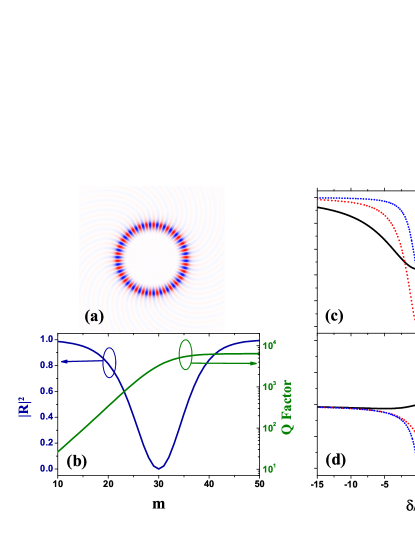
Figure 1: (color online) (a) The electric field distribution when a cylinder cavity is critical coupling with $m=30$ cylinder wave, and detuning $\delta$ $=0$. (b) The normalized reflectivity and the total Q factor against the angular number $m$, with the refractive index $n=1.45+0.000117i$. (c) and (d) are the intensity and phase of outgoing field for different coupling condition, with $\kappa_{1}/\kappa_{0}=0.2$ (Red Solid lines), $1.0$ (Blue Dashed lines) and $5.0$ (Black Dotted lines).

In above formulas, there are singularities at $z=z_{0}$ where

$$n^{p}J_{m}^{\prime}(nz_{0})H_{m}^{(1)}(z_{0})-J_{m}(nz_{0})H_{m}^{(1)\prime}(z_{0})=0.$$ (3)

This corresponds to the quasi-bound eigenmodes (WGMs) with dimensionless eigenfrequency ($kr_{c}=z_{0}$), which is a complex number. When the material refractive index $n$ is real, i.e. there no material absorption, we can write $z_{0}=z_{0}^{r}-i\kappa_{0}$ with $z_{0}^{r}$ and $\kappa_{0}$ are real numbers. Here, $\kappa_{0}$ is the pure radiation loss of WGM, which corresponds to the width of the resonance in spectrum as $\kappa_{0}=z_{0}^{r}/2Q_{0}$ with $Q_{0}$ is the radiation quality factor.

For nearly resonant frequency $z=z_{0}+\Delta$ ($|\Delta|\ll|z_{0}|)$, by expanding Eq. (3) to the first order of $\Delta$, we can approximately obtain

$$n^{p}J_{m}^{\prime}(nz)H_{m}^{(1)}(kz)-J_{m}(nz)H_{m}^{(1)\prime}(z)\approx F(z_{0})\Delta\text{,}$$ (4)

with $F(z_{0})=(n^{p-1}-1)[(nJ_{m}^{\prime}(nz_{0})H_{m}^{(1)\prime}(z_{0})+\frac{m(m-1)}{z_{0}^{2}}J_{m}(nz_{0})H_{m}^{(1)}(z_{0})]-(n^{p+1}-1)J_{m}(nz_{0})H_{m}^{(1)}(z_{0})$.

For the real materials, the non-radiation linear loss should be taken into account. For example, the material absorption can be considered in the characterize equation by adding a small complex number ($n_{i}\ll n$) to the refractive index as $\widetilde{n}=n+in_{i}$. For a monochromatic light with $z=z_{0}^{r}-\delta$, we have $\widetilde{n}z=(n+in_{i})(z_{0}^{r}-\delta)\approx n(z_{0}-\delta-i\kappa_{0}-i\kappa_{1})$ with $\kappa_{1}=z_{0}n_{i}/n$ denotes the non-radiation loss. Substitute $\Delta=i(i\delta+\kappa_{0}+\kappa_{1})$ into Eq. (4), Eq. (1), and Eq. (2). Under the high-Q mode ($\kappa_{0}\ll z_{0}^{r}$) and near resonance ($\delta\ll z_{0}^{r}$) conditions, and with the approximation that most of WGM energy is confined inside the cavity, we can get

$$a_{m}(\delta) =\frac{1}{i\delta+\kappa_{0}+\kappa_{1}}\frac{-4}{\pi z_{0}^{r}F(z_{0}^{r})}c_{m}\text{,}$$ (5)

$$b_{m}(\delta) =-\frac{i\delta-\kappa_{0}+\kappa_{1}}{i\delta+\kappa_{0}+\kappa_{1}}\frac{F^{\ast}(z_{0}^{r})}{F(z_{0}^{r})}c_{m}\text{.}$$ (6)

On the other hand, the standard input-output formulation for a cavity mode is Walls

$$\frac{d}{dt}E_{m}=(-i\delta-\kappa_{0}-\kappa_{1})E_{m}+\sqrt{2\kappa_{0}}E_{m}^{in}\text{,}$$ (7)

where $E_{m}$ is the cavity mode field, $E_{m}^{in}$ is the incoming field in the form of radial inward cylinder waves $H_{m}^{(2)}(z_{0})$, and the output field is $E_{m}^{out}=-E_{m}^{in}+\sqrt{2\kappa_{0}}E_{m}.$ When the system is in the steady state, $\frac{d}{dt}E_{m}=0$ should be satisfied, thus

$$E_{m}=\frac{\sqrt{2\kappa_{0}}}{i\delta+\kappa_{0}+\kappa_{1}}E_{m}^{in}\text{,}$$ (8)

and the output field is

$$E_{m}^{out}=-\frac{i\delta-\kappa_{0}+\kappa_{1}}{i\delta+\kappa_{0}+\kappa_{1}}E_{m}^{in}\text{.}$$ (9)

Comparing those equations with Eq. (5) and Eq. (6), the cavity and outgoing fields deduced by input-output formulation are consistent with the results derived by boundary conditions, only different in constants. The conversion relationships between two sets of formulas are $a_{m}=\frac{1}{\sqrt{2\kappa_{0}}}\frac{-4}{\pi z_{0}^{r}F^{\ast}(z_{0}^{r})}E_{m}$, $b_{m}=E_{m}^{out}$, and $c_{m}=E_{m}^{in}\frac{F(z_{0}^{r})}{F^{\ast}(z_{0}^{r})}$.

For the case of the near field coupler, the cavity field reads CMT3

$$E_{m}=\frac{\sqrt{2\kappa_{e}}}{i\delta+\kappa_{i}+\kappa_{e}}E_{m}^{in},$$ (10)

where $\kappa_{i}$ is intrinsic loss including radiation and absorption losses, and $\kappa_{e}$ is external loss induced by coupler. Comparing with Eq. (8), the free space and near field coupling manners are similar, with $\kappa_{0}$ and $\kappa_{1}$ replaced by $\kappa_{i}$ and $\kappa_{e}$.

From Eq. (8), the extremum of cavity field emerges when $\partial E/\partial\kappa_{0}=0$, i.e. $\kappa_{0}=\kappa$ with $\delta=0$. Similar to the case of a near field waveguide coupling to WGMs, there are three coupling regimes: under coupling regime $\kappa_{0}<\kappa_{1}$; critical coupling regime $\kappa_{0}=\kappa_{1}$; and over coupling regime $\kappa_{0}>\kappa_{1}$. The electric field distribution in Fig. 1(a) clearly shows the excitation of WGM at critical coupling by an inward cylinder wave $H_{30}^{(2)}(kr)e^{i30\phi}$ with the spiral-like propagation. No reflection wave is excited in this case, which means all energy is perfectly absorbed by the cavity. Fig. 1(c) and (d) are the intensity and the phase of outgoing wave against the detuning in three regimes. In the under and over coupling regime, the energy transfer efficiency without detuning is low. Moreover, the phase of the outgoing wave is strongly changed by the WGM in the over coupling regime with small detuning value, while there is only small perturbation for under coupling regime.

In the case of near field coupler, the extra coupling loss $\kappa_{e}$ can be controlled by simply adjusting the gap between coupler and cavity, while $\kappa_{i}$ is an intrinsic parameter that does not change. Differently, in the free space coupling case, $\kappa_{1}$ is an intrinsic parameter determined by material and fabrication which is almost a constant for WGMs. It is only possible to change $\kappa_{0}$ by change the cavity size or boundary shape. As shown in Fig. 1(b), the Q-factor [$Q=kr_{c}/2(\kappa_{0}+\kappa_{1})$] and the outgoing intensity change against $m$ with $n=1.45+0.000117i$. The Q-factor increases with the increasing $m$ and shows a saturation value of about $6\times 10^{3}$. The critical coupling ($\kappa_{0}\approx\kappa_{1}$) happens when $m=30$, corresponding to a specific cavity size ($r_{c}\approx m/nk$). For larger or smaller cavity size, the coupling efficiency reduces.

II.2 Gaussian Beam

Figure 2: (color online) (a) Schematic illustration of a Gaussian beam incident to a whispering gallery microcavity. The direction of beam is defined by $\theta_{0}$, and the location of center is $(r_{0},\phi_{0})$ in the cylinder coordinator. (b) The electric field intensity distribution when the incident Gaussian beam is resonant with the WGM, with $kr_{c}=30.10,$ $r_{0}=1.1r_{c}$, $\phi_{0}=\pi/2$ and $\theta_{0}=0.$

Gaussian beam is most widely applied in experiments. Thus we use this beam in following studies for realistic consideration. Supposing a Gaussian beam centered at ($x_{0},y_{0}$) with intensity $I=1$ and propagation along $x$-axis with the waist width $w$, the electric field at the waist is

$$G(x_{0},y)=e^{-\frac{(y-y_{0})^{2}}{w^{2}}}$$ (11)

Correspondingly, the angular spectrum is

$$\widetilde{G}(\theta) =\frac{1}{2\pi}\int_{-\infty}^{\infty}e^{-iyk\mathrm{sin}\theta}e^{-\frac{y^{2}}{w^{2}}}dy$$

$$=\frac{w}{2\sqrt{\pi}}e^{-\frac{k^{2}w^{2}}{4}\mathrm{sin}^{2}\theta}\text{,}$$ (12)

with $\theta\in(-\frac{\pi}{2},\frac{\pi}{2}).$ So, in the cylinder coordinator in Fig. 2(a), the field distribution can be expressed as

$$E(r,\phi)=\int_{-k}^{k}\frac{w}{2\sqrt{\pi}}e^{-\frac{k^{2}w^{2}}{4}\mathrm{sin}^{2}\theta}e^{ik(\mathrm{sin}\theta y+\mathrm{cos}\theta x)}d(k\mathrm{sin}\theta),$$ (13)

where

$$x =r\mathrm{cos}(\phi+\theta_{0})-r_{0}\mathrm{cos}(\phi_{0}+\theta_{0}),$$ (14)

$$y =r\mathrm{sin}(\phi+\theta_{0})-r_{0}\mathrm{sin}(\phi_{0}+\theta_{0}).$$ (15)

Substituting them to the Eq. (13) and employing the Jacobi-Anger expansion,

$$e^{ikr\mathrm{cos}(\phi+\theta_{0}-\theta)}=\underset{m=-\infty}{\overset{\infty}{{\textstyle\sum}}}J_{m}(kr)e^{im[\pi/2-(\phi+\theta_{0}-\theta)]},$$ (16)

we can derive the coefficient of Gaussian beam in inward cylinder waves expansion

$$c_{m}=\frac{e^{im(\pi/2-\theta_{0})-ikq-\frac{[kr_{0}d-m]^{2}}{k^{2}w^{2}+i2kq}}}{2\sqrt{1+i\frac{2q}{kw^{2}}}},$$ (17)

in the limit of $kw\gg 1$ and $d=r_{0}\mathrm{sin}(\phi_{0}+\theta_{0})$ and $q=r_{0}\mathrm{cos}(\phi_{0}+\theta_{0})$. Here, only the part of $\mathrm{sin}\theta\ll 1$ contributes in the integral, and the approximation is applied

$$\mathrm{cos}\theta=\sqrt{1-\mathrm{sin}^{2}\theta}\approx 1-\frac{1}{2}\mathrm{sin}^{2}\theta\text{.}$$ (18)

Substituting the coefficients to Eq. (1) and (2), the intracavity field and outgoing field can be solved analytically for a cylinder cavity. For example, Fig. 2(b) shows the near field distribution when a Gaussian beam incident to the cavity with the on-resonance frequency to WGM with $m=40$. Obviously, most energy are directly transmitted. Only a small portion of energy can be coupled into the cavity field. By integrating the Poynting vector of the electromagnetic field, we can calculate the power (energy flux) contained in the Gaussian beam

$$P_{G}=\sqrt{\frac{\pi}{2}}\frac{kw}{2\omega\mu},$$ (19)

where $\omega$ is angular frequency, and $\mu$ is relative permeability. Power of normalized cylinder wave $H_{m}^{(1(2))}(kr)e^{im\phi}$ is

$$P_{m}=\frac{2}{\omega\mu}.$$ (20)

Therefore, the ratio of power contained in the $m$-th cylinder waves to that in the Gaussian beam is

$$\eta_{m}=\left|c_{m}\right|^{2}\frac{P_{m}}{P_{G}}.$$ (21)

From Eq. (17), $\eta_{m}$ is maximal when $q=0$ and $d=m/k$. The first condition guarantees the smallest expansion of cylinder waves in momentum space ($m$). The second condition corresponds to the phase matching condition that the momentum of the pump beam ($kd$) should be equal to the momentum of the WGM ($m$). In practical applications, we can manipulate the beam position d to satisfy the conditions, then

$$\eta_{max}=\sqrt{\frac{2}{\pi}}\frac{1}{kw}.$$ (22)

Therefore, the rate of power transfer from a Gaussian beam to the cavity WGM is limited to $\eta_{max}$. Under the paraxial approximation, the waist $w$ of a Gaussian beam should be larger than $4/k$, i.e. $kw\geq 4$, corresponding to the energy transferring rate $\eta_{m}\leq 0.2$ for a cylinder cavity.

III Deformed Cylinder

III.1 General Model

When the cavity boundary is slightly deformed ARC1 ; ARC2 ; ARC3 ; ARC4 ; ARC5 ; ARC6 ; ARC7 ; ARC8 ; ARC9 ; uni2 ; uni3 ; uni4 ; uni5 ; uni7 ; uni8 or small perturbations are introduced to the cavity uni1 ; uni6 , highly directional emission can be obtained. Because the boundaries of ARCs are not regular, different momentum (m) components can couple to each other. In addition, WGMs always exist in pairs, clockwise ($A_{c}$) and anti-clockwise ($A_{a}$) traveling modes, in a circular-like shape microcavity, then the general Hamiltonian of ARC reads

$$\mathcal{H}=\mathcal{H}_{modes}+\mathcal{H}_{int}+\mathcal{H}_{pump}.$$ (23)

Here,

$$\mathcal{H}_{modes}=\sum_{j}\hbar\delta_{j}(A_{j,c}^{{\dagger}}A_{j,c}+A_{j,a}^{{\dagger}}A_{j,a})$$ (24)

represents the energy of cavity modes, with $\delta_{j}$ is the frequency difference between cavity mode and excitation laser, and $A_{j,c}^{{\dagger}}(A_{j,c})$ is the creation (annihilation) operator of cavity mode. The coupling between different modes is

$$\mathcal{H}_{int} =\sum_{j}\sum_{k>j}(g_{j,k,c}A_{j,c}^{{\dagger}}A_{k,c}+g_{j,k,a}A_{j,a}^{{\dagger}}A_{k,a}+h.c.)$$

$$+\sum_{j,k}(\beta_{j,k}A_{j,c}^{{\dagger}}A_{k,a}+h.c.),$$ (25)

where $\beta_{j,k}$ is the coupling coefficient between counter propagation WGMs and $g_{j,k,a(c)}$ is the coupling coefficient between co-propagation modes. The external pumping on modes is given by

$$\mathcal{H}_{pump}=\sum_{j,m}(ih_{j,m,c}A_{j,c}^{{\dagger}}u_{m}^{in}+ih_{j,m,a}A_{j,a}^{{\dagger}}u_{-m}^{in}+h.c.).$$ (26)

Here, $h_{j,m,c}$ is the coupling strength of the cavity mode to the outside cylinder waves, with $m=1\cdots\infty$, where the external incoming field and outgoing field are represented by cylinder waves as ${\textstyle\sum}u_{m}^{in}e^{i\varphi_{m}}H_{m}^{(2)}(kr)e^{-im\phi}$ and ${\textstyle\sum}u_{m}^{out}e^{-i\varphi_{m}}H_{m}^{(1)}(kr)e^{-im\phi}$ with $e^{-i2\varphi_{m}}=-H_{m}^{(2)}(kr_{c})/H_{m}^{(1)}(kr_{c})$. Actually, $A_{c}$ and $A_{a}$ are time reversal to each other, so the coupling coefficients satisfy $g_{j,k,c}=g_{j,k,a}^{\ast}=g_{j,k}$ and $h_{j,m,c}=h_{j,m,a}^{\ast}=h_{j,m}$.

Here, we only concern about the ARCs with smooth boundary and small deformation which can support high-Q WGMs. Then we can omit the coupling between counter propagation WGMs ($\beta_{i,j}=0$) and the direct scattering induced transition between incoming and outgoing cylinder waves. Thus the Heisenberg equation of cavity field are written as

$$\frac{d}{dt}A_{j,c} =-i\sum\limits_{k>j}g_{j,k}A_{k,c}-i\sum\limits_{k<j}g_{k,j}^{\ast}A_{k,c}$$

$$-\chi_{j}A_{j,c}+\sum\limits_{m}h_{j,m}u_{m}^{in},$$ (27)

where $\chi_{j}=i\delta_{j}+\kappa_{j,0}+\kappa_{j,1}$, $\kappa_{j,0}=\sum_{m}\left|h_{j,m}\right|^{2}/2$ and $\kappa_{j,1}$ are intrinsic radiation loss and non-radiation loss, respectively. Supposing there is only one high-Q WGM with $j=1$ near resonance of the excitation, and other modes are low-Q or largely detuned, we can adiabatic eliminate the fast varying terms by $\frac{d}{dt}A_{j,c}=0$ for $j\geq 2$, i.e.

$$A_{j,c}|_{j\geq 2}=-i\frac{g_{1,j}^{\ast}}{\chi_{j}}A_{1,c}+\underset{m=1}{\overset{\infty}{{\textstyle\sum}}}\frac{h_{j,m}}{\chi_{j}}u_{m}^{in}\text{.}$$ (28)

Therefore,

$$\frac{d}{dt}A_{1,c}=-\widetilde{\chi}_{1}A_{1,c}+\underset{m=1}{\overset{\infty}{{\textstyle\sum}}}\widetilde{h}_{1,m}u_{m}^{in}\text{.}$$ (29)

Here, $\widetilde{\chi}_{1}=\chi_{1}+\kappa_{e}+i\delta_{e}$ with $\kappa_{e}=\sum_{j\geq 2}\frac{\kappa_{j,0}+\kappa_{j,1}}{\left|\chi_{j}\right|^{2}}\left|g_{1,j}\right|^{2}$ and $\delta_{e}=-\sum_{j\geq 2}\frac{\delta_{j}}{\left|\chi_{j}\right|^{2}}\left|g_{1,j}\right|^{2}$, corresponding to the extra loss and frequency shift induced by low-Q modes, and $\widetilde{h}_{1,m}=h_{1,m}-i\sum_{j\geq 2}g_{1,j}\frac{h_{j,m}}{\chi_{j}}$ are effective coupling coefficients to outside for high-Q WGM. Denoting the coupling efficiencies and the incoming field by vectors $\vec{h}=\{\widetilde{h}_{1,m}\}$ and $\vec{u}=\{u_{m}^{in}\}$ with $m=1\cdots\infty$, the cavity field of steady state becomes

$$A_{1,c}=\xi\left|\vec{h}\right|\left|\vec{u}\right|/\widetilde{\chi}_{1},$$ (30)

where $\xi=\vec{h}\cdot\vec{u}/\left|\vec{h}\right|\left|\vec{u}\right|$ is the beam matching parameter. The output for arbitrary incoming field reads

$$u_{m}^{out}=-u_{m}^{in}+f_{m}A_{1,c}+\sum_{j\geq 2}\sum_{m^{\prime}}\frac{h_{j,m}^{\ast}h_{j,m^{\prime}}}{\chi_{j}}u_{m^{\prime}}^{in},$$ (31)

where $f_{m}=h_{1,m}^{\ast}-i\sum_{j\geq 2}\frac{g_{1,j}^{\ast}}{\chi_{j}}h_{j,m}^{\ast}$ corresponds to the radiation of $A_{1,c}$.

From Cauchy-Schwartz inequality, $\left|\xi\right|\leq 1$, the maximum of matching can be achieved only when

$$\vec{u}\propto\vec{h}^{\ast}/\left|\vec{h}\right|.$$ (32)

This corresponds to the optimal beam to excite the WGM $E_{inc}(r,\phi)\propto\sum_{m}e_{m}^{i\varphi_{m}}\widetilde{h}_{1,m}^{\ast}H_{m}^{(2)}(kr)e^{-im\phi}$, which is the reverse of the radiation of anti-clockwise WGM $E_{a}^{rad}(r,\phi)\propto\sum_{m}\widetilde{h}_{1,m}e^{-i\varphi_{m}}H_{m}^{(1)}(kr)e^{im\phi}$, meaning that the optimal excitation of clockwise WGM can be achieved by the reverse of the radiation of anti-clockwise WGM.

When on resonance, the cavity field reads $A_{1,c}=\xi\left|\vec{h}\right|\left|\vec{u}\right|/(\kappa_{1,0}+\kappa_{1,1}+\kappa_{e})$, and the energy transferring depends on both $\xi$ and $\left|\vec{h}\right|/(\kappa_{1,0}+\kappa_{1,1}+\kappa_{e})$. All the parameters mentioned above can not be solved analytically because of the irregular boundary shape. Realistic details about the free space coupling should be solved by numerical simulation fscshu . In the following, we analytically solve the free space coupling to ARCs by an abstract model without the specific boundary shape. In this simplified model, we assume directional emission is in the form of Gaussian beam ignoring the specific boundary of a ARC. The general underlying mechanism and basic properties are revealed with several reasonable approximations of a near circular boundary shape.

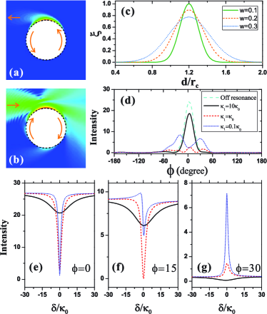
Figure 3: (color online) (a) Field distribution of directional emission of anti-clockwise WGM in a near circular cavity (The field is shown in Logarithm scale, and the intracavity field is not shown since the exact boundary shape is not known in our abstract model). The emission is in the form of Gaussian beam with $d_{t}=1.2r_{c}$, $w_{t}=0.1r_{c}$ and direction is shown by arrows. (b) Field distribution when an on-resonance Gaussian beam coupling to the cavity in the over coupling regime with $\kappa_{1}=0.1\kappa_{{0}}$, $d=1.2$, $w=0.2r_{c}$ and direction is shown by arrows. (c) Beam matching parameters against the $d$ for different $w$. (d) The far field intensity of outgoing wave when a Gaussian beam incident to a cylinder, for excitation frequency off-resonance and on-resonance at difference coupling conditions. (e), (f) and (g) are spectra detected at different angle ($\phi$) in far field.

III.2 Coupling Through Barrier Tunneling

In a very slightly deformed ARC, the coupling between high-Q and low-Q modes are weak, and the directional emission is mainly due to the direct tunneling Creagh . The center of the emission beam is departed from the boundary, as a result of barrier tunneling Tomes . We assume that the parameters of emission Gaussian beam are $d_{t}=1.2r_{c}$, $w_{t}=0.1r_{c}$ and direction along $x$-axis, as shown in Fig. 3(a). Thus, the coupling coefficients can be solved from the mode emission

$$h_{1,m}=\mathfrak{h}_{0}e^{-im\pi/2-\frac{[kd_{t}-m]^{2}}{k^{2}w_{t}^{2}}+i\varphi_{m}},$$ (33)

where $\mathfrak{h}_{0}=\sqrt{\kappa_{0}/\sqrt{\frac{\pi}{2}}\frac{kw}{2}}$, corresponding to the normalization ${\sum}\left|h_{1,m}\right|^{2}=2\kappa_{0}$.

We discussed the coupling in detail using a Gaussian beam from left with $\theta_{0}=0$ and on-resonance to a high-Q mode of $kr_{c}=31.1$. Firstly, we calculated the beam matching parameter $\xi$ versus the beam position $d$ for different beam widths $w$, as shown in Fig. 3(c). The result shows that good match with $\xi>0.8$ can be easily realized with good fault tolerant to the imperfect focus or align of beam in experiments. In the near integrated system, we can neglect the coupling to other low-Q modes $(\kappa_{0}^{1,c}+\kappa_{1}^{1,c}\gg\kappa_{e})$, then $A_{c}\approx\sqrt{2\kappa_{1,0}}/\left(\kappa_{1,0}+\kappa_{1,1}\right)$. Similar to the cylinder case, the critical coupling with $\kappa_{1,0}=\kappa_{1,1}$ guarantees the maximum energy transfer.

With these approximations, we can calculate the far field distributions by substituting parameters into Eq. (30). The far field distributions at different coupling regime are shown in Fig. 3(d) with $w=0.2r_{c}$. At critical coupling, the outgoing energy is great reduced but larger than $0$ as a result of imperfect matching. In under coupling, there is a small reduction of energy in all directions. However, in over coupling regime, the peak at $\phi=0$ is split into two peaks, which is attributed to the interference between the transmitted beam and the emission of the cavity mode, as a result of the strong phase shift at the over coupling regime.

The spectra are also calculated (Figs. 3(e), 3(f) and 3(g)) in different far field angles. It is revealed that the line shapes strongly depend on the positions of detectors. At $\phi=0^{\circ}$, the resonances shows regular Lorentz-shape dips similar to traditional near field coupler. In contrast with Fig. 1(c), similar dip depths are given in the over and critical coupling condition regimes, which indicates that the dip depth can not tell us the energy transfer rate in the free space coupling. Asymmetric line shapes (Fano-like and EIT-like) are observed at $\phi=15^{\circ}$ and $30^{\circ}$, as a result of multiple cylinder waves interference formalized in Eq. (31).

III.3 Coupling Through Refraction

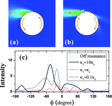
Figure 4: (color online) (a) Field distribution of directional emission of anti-clockwise WGM in a near circular cavity (The field is shown in normal scale, and the intracavity field is not shown since the exact boundary shape is not known in our abstract model). The emission is in the form of Gaussian beam with $d_{r}=0.9r_{c}$, $w_{r}=0.1r_{c}$ and direction is shown by arrows. (b) The field distribution when an on-resonance Gaussian beam coupling to the cavity in the over coupling regime with $\kappa_{1}=0.1\kappa_{0}$, $d=0.9$, $w=0.2r_{c}$ and direction is shown by arrows. (c) The far field intensity of outgoing wave when a Gaussian beam is incident to the ARC with Gaussian beam emission, for off-resonance and on-resonance under different coupling conditions.

When the degree of deformation is large, the directional emission is mainly due to the radiation from low-Q modes. This process is also known as the dynamical tunneling in the study of ARC, where rays in high-Q mode tunnel into chaotic sea and refracted out at some specific region in phase space ARC5 ; ARC6 . The center of Gaussian beam should be adjusted on the cavity as a result of refraction image . For the refraction dominated emission, the extra loss induced by low-Q mode is much larger than the intrinsic radiation loss ( i.e. $\kappa_{e}\gg\kappa_{0}$), thus we can neglect the direct tunneling loss. Assuming the emission is Gaussian beam with the parameters $d_{r}=0.9r_{c}$, $w_{r}=0.1r_{c}$ and direction along $x$-axis (Fig. 4(a)), we have

$$\sum_{j\geq 2}\frac{g_{1,j}}{\chi_{j}}h_{j,m}e^{-i\varphi_{m}}=\mathfrak{h}_{e}e^{-im\pi/2-\frac{[kd_{t}-m]^{2}}{k^{2}w_{t}^{2}}}.$$ (34)

Here, $\mathfrak{h}_{e}=\sqrt{\kappa_{e}/\sqrt{\frac{\pi}{2}}\frac{kw}{2}}$ with $\kappa_{e}=\frac{1}{2}\sum_{m\geq 2}\frac{\left|g_{1,m}\right|^{2}\left|h_{m,m}\right|^{2}}{\left|\chi_{m}\right|^{2}}$. In addition, the interactions between low-Q modes are not taken into consideration. We also assume the deformation just slightly influence the low-Q modes for simplicity, thus $h_{j,m}=0$ if $j\neq m$. Therefore

$$\frac{g_{1,m}}{\chi_{m}}h_{m,m}=\mathfrak{h}_{e}e^{-im\pi/2-\frac{[kd_{t}-m]^{2}}{k^{2}w_{t}^{2}}+i\varphi_{m}}.$$ (35)

Similar to the procedure in previous section, we solved the outgoing field when a Gaussian beam incident from left with $\theta_{0}=0$, $w=0.2r_{c}$, $d=0.9r_{c}$ and on-resonance to a high-Q mode with $kr_{c}=31.1$. As shown in Figs. 4(b) and 4(c), the maximal far field intensity is located away from $\phi=0$ as a result of the refraction of incident beam. The far field distribution is similar to the case of tunneling coupling, and the EIT or asymmetric line shapes are presented in the spectra (not shown here).

IV Discussion

According to the above analysis, the coupling to high-Q WGMs through free space can be efficient. For the cylinder wave, the largest coupling efficiency can be achieved under the phase matching condition, and the maximum is limited by waist width of a focused Gaussian beam, as the ratio of power contained in the cylinder wave is limited. For a deformed cavity, the efficiency can be higher since the pump Gaussian beam can be well matched to the directional emission beam.

The energy transferred to the cavity is also determined by the coupling regime, i.e. the ratio of radiation loss to non-radiation loss. The strongest coupling happens when $\kappa_{0}\approx\kappa_{1}$. The radiation loss $\kappa_{0}$ decreases exponentially with the increasing of cavity size, but the non-radiation loss $\kappa_{1}$ is almost constant. Therefore, in a large cavity, $\kappa_{0}$ is much greater than $\kappa_{1}$, which will give rise to very inefficient coupling. This limitation can be removed in the deformed cavity, as $\kappa_{0}$ can be tuned by adjusting the deformation. Usually, a large degree of deformation can also lead to better directionality of cavity emission, thus better beam matching. Therefore, we can always tune the deformation degree to achieve the largest energy transfer rate, similar to the tuning of gap between near field coupler and microcavity.

In contrast to near field coupler to microcavity, the asymmetric line shapes are universal in free space coupling to WGMs uni8 ; fscshu . In more realistic cases, maybe multiple high-Q modes near to each other in spectrum are involved, and then the interactions between high-Q modes are enhanced by the low-Q modes mediated mode-mode interaction. From the view of ray dynamics in ARC, the high-Q modes usually correspond to regular period or quasi-period orbits. Due to dynamical tunneling, the high-Q modes can couple to chaotic modes which correspond to chaotic ray trajectories. Therefore, the chaotic sea mediated the indirect coupling between separated regular orbits in phase space (high-Q modes), which is also known as chaos assisted tunneling ray3 ; CAT1 ; CAT2 . Similar to the case of waveguide coupled microcavity EIT3 ; Fano1 , we can expect more profound asymmetric spectra when take more high-Q modes into consideration.

V Conclusion

In summary, we present the theoretical study of the free space coupling to high-Q WGMs in both regular and deformed microcavities. The coupling by free space beam depends on the phase matching and beam matching conditions in regular cylinder cavities and ARCs, respectively. Three coupling regimes of free space coupling are discussed: the cavity should work near the critical coupling regime for high efficiency energy transfer. In cylinder cavity, the maximum energy transfer efficient is limited, and critical coupling can only be achieved with specific cavity size. The ARCs not only give good beam matching between focused Gaussian beam and highly directional emission, but also enable the tuning of the cavity degree of deformation to achieve critical coupling. Therefore, the efficiency approaching unity is possible in realistic experiments of free space coupling to unidirectional emission cavity. It is found that the asymmetric spectra or peak like spectra instead of the Lorentz-shape dip is universal in spectra, and the coupling efficiency cannot be estimated from the absolute depth of dip. Our results provide guidelines for free space coupling to high-Q WGMs, which will be valuable for further experiments and applications of WGMs based on free space coupling.

VI Acknowledgement

We thank Prof. Hailin Wang and Prof. Kyungwon An for discussions and comments. This work was supported by the 973 Programs (No. 2011CB921200), the National Natural Science Foundation of China (NSFC) (No. 11004184), the Knowledge Innovation Project of the Chinese Academy of Sciences (CAS). F.-J. Shu is supported by the Foundation of He’nan Educational Committee (No. 2011A140021) and the Young Scientists Fund of the National Natural Science Foundation of China (Grant No. 11204169).

References

- (1) Lord Rayleigh, Phil. Mag. 20, 1001 (1910).
- (2) R. D. Richtmyer, J. Appl. Phys. 10, 391 (1939)
- (3) F. Vollmer, and S. Arnold, Nature Methods 5, 591 (2008).
- (4) L. He, S. K. Ozdemir, and L. Yang, Laser & Photonics Reviews, In press (2012).
- (5) P. Del’Haye, A. Schliesser, O. Arcizet, T. Wilken, R. Holzwarth, and T. J. Kippenberg, Nature 450, 1214 (2007).
- (6) T. Aoki, B. Dayan, E. Wilcut, W. P. Bowen, A. S. Parkins, T. J. Kippenberg, K. J. Vahala, and H. J. Kimble, Nature 443, 671 (2006).
- (7) Y. S. Park, and H. Wang, Nature Phys. 5, 489-493 (2009).
- (8) E. Verhagen, S. Deleglise, S. Weis, A. Schliesser, and T. J. Kippenberg, Nature 482, 63 (2012).
- (9) G. Mie, Ann. Phys. (Leipzig) 330, 377 (1908).
- (10) H. Moyses Nussenzveig, Sci. Am. 306(1), 68 (2012)
- (11) S. X. Qian, J. B. Snow, H.-M. Tzeng, R. K. Chang, Science 231, 486 (1986)
- (12) V. B. Braginsky, M. L. Gorodetsky, V. S. Ilchenko, Phys. Lett. A 137, 393 (1989).
- (13) S. L. McCall, A. F. J. Levi, R. E. Slusher, S. J. Pearton, R. A. Logan, Appl. Phys. Lett. 60, 289 (1992).
- (14) H. J. Moon, Y. T. Chough, K. An, Phys. Rev. Lett. 85, 3161 (2000).
- (15) D. K. Armani, T. J. Kippenberg, S. M. Spillane, K. J. Vahala, Nature 421, 925 (2003).
- (16) M. L. Gorodetsky, and V. S. Ilchenko, Opt Commun 113, 133 (1994).
- (17) M. Cai, O. Painter, and K. J. Vahala, Phys. Rev. Lett. 85, 74 (2000).
- (18) Y.-Z. Yan, C.-L. Zou, S.-B. Yan, F.-W. Sun, Z. Ji, J. Liu, Y.-G. Zhang, L. Wang, C.-Y. Xue, and W.-D. Zhang, Opt. Express 19, 5753 (2011).
- (19) F.-J. Shu, C.-L. Zou, and F.-W. Sun, Opt. Lett. 37, 3123 (2012).
- (20) B. E. Little, J. P. Laine, and H. A. Haus, J. Lightwave Technol. 17, 704 (1999).
- (21) A. Yariv, Electronics Letters 36, 321 (2000).
- (22) C.-L. Zou, Y. Yang, C.-H. Dong, Y.-F. Xiao, X.-W. Wu, Z.-F. Han, and G.-C. Guo, J. Opt. Soc. Am. B 25, 1895 (2008).
- (23) M. F. Yanik, W. Suh, Z. Wang, and S. Fan, Phys. Rev. Lett. 93, 233903 (2004).
- (24) K. Totsuka, N. Kobayashi, and M. Tomita, Phys. Rev. Lett. 98, 213904 (2007).
- (25) C.-H. Dong, C.-L. Zou, Y.-F. Xiao, J.-M. Cui, Z.-F. Han, and G.-C. Guo, J. Phys. B 42, 215401 (2009).
- (26) B.-B. Li, Y.-F. Xiao, C.-L. Zou, Y.-C. Liu, X.-F. Jiang, Y.-L. Chen, Y. Li, and Q. Gong, Appl. Phys. Lett. 98, 021116 (2011).
- (27) B.-B. Li, Y.-F. Xiao, C.- L. Zou, X.-F. Jiang, Y.-C. Liu, F.-W. Sun, Y. Li, and Q. Gong, Appl. Phys. Lett. 100, 021108 (2012).
- (28) A. Chiba, H. Fujiwara, J.-i. Hotta, S. Takeuchi, and K. Sasaki, Appl. Phys. Lett. 86, 261106 (2005).
- (29) C. Dong, C. Zou, J. Cui, Y. Yang, Z. Han, and G. Guo, Chin. Opt. Lett. 7, 299 (2009).
- (30) A. Mekis, J. U. Nöckel, G. Chen, A. D. Stone, and R. K. Chang, Phys. Rev. Lett. 75, 2682 (1995).
- (31) C. Gmachl, F. Capasso, E. E. Narimanov, J. U. Nöckel, A. D. Stone, J. Faist, D. L. Sivco, and A. Y. Cho, Science 280, 1556 (1998).
- (32) S.-B. Lee, J.-H. Lee, J.-S. Chang, H.-J. Moon, S. W. Kim, and K. An, Phys. Rev. Lett. 88, 033903 (2002).
- (33) S. Lacey, H. Wang, D. H. Foster, and J. U. Nöckel, Phys. Rev. Lett. 91, 033902(2003).
- (34) Y.-F. Xiao, C.-H. Dong, Z.-F. Han, G.-C. Guo, and Y.-S. Park, Opt. Lett. 32, 644 (2007).
- (35) T. Harayama, T. Fukushima, P. Davis, P. O. Vaccaro, T. Miyasaka, T. Nishimura, and T. Aida, Phys. Rev. E 67, 015207 (2003).
- (36) W. Fang, A. Yamilov, and H. Cao, Phys. Rev. A 72, 023815 (2005).
- (37) M. Lebental, J. S. Lauret, R. Hierle, and J. Zyss, Appl. Phys. Lett. 88, 031108 (2006).
- (38) Y.-F. Xiao, C.-H. Dong, C.-L. Zou, Z.-F. Han, L. Yang, and G.-C. Guo, Opt. Lett. 34, 509 (2009).
- (39) J. U. Nöckel and A. D. Stone, Nature 385, 45 (1997).
- (40) H. G. L. Schwefel, N. B. Rex, H. E. Tureci, R. K. Chang, A. D. Stone, T. Ben-Messaoud, and J. Zyss, J. Opt. Soc. Am. B 21, 923 (2004).
- (41) V. A. Podolskiy and E. E. Narimanov, Opt. Lett. 30, 474 (2005).
- (42) S. Shinohara, T. Fukushima, and T. Harayama, Phys. Rev. A 77, 033807 (2008).
- (43) S. B. Lee, J. Yang, S. Moon, J. H. Lee, K. An, J. B. Shim, H. W. Lee, and S. W. Kim, Phys. Rev. A 75, 011802 (2007).
- (44) J. Wiersig and M. Hentschel, Phys. Rev. A 73, 031802 (2006).
- (45) J. Wiersig, and M. Hentschel, Phys. Rev. Lett. 100, 033901 (2008).
- (46) Q. Song, W. Fang, B. Liu, S.-T. Ho, G. S. Solomon, and H. Cao, Phys. Rev. A 80, 041807 (2009).
- (47) C. Yan, Q. J. Wang, L. Diehl, M. Hentschel, J. Wiersig, N. Yu, C. Pflugl, F. Capasso, M. A. Belkin, T. Edamura, M. Yamanishi, and H. Kan, Appl. Phys. Lett. 94, 251101 (2009).
- (48) S. Shinohara, M. Hentschel, J. Wiersig, T. Sasaki, and T. Harayama, Phys. Rev. A 80, 031801 (2009).
- (49) C.-L. Zou, F.-W. Sun, C.-H. Dong, X.-W. Wu, J.-M. Cui, Y. Yang, G.-C. Guo, Z.-F. Han, arXiv:0908.3531.
- (50) X.-F. Jiang, Y.-F. Xiao, C.-L. Zou, L. He, C.-H. Dong, B.-B. Li, Y. Li, F.-W. Sun, L. Yang, and Q. Gong, Adv. Mater. 24, OP260 (2012).
- (51) Q. J. Wang, C. Yan, N. Yu, J. Unterhinninghofen, J. Wiersig, C. Pflugl, L. Diehl, T. Edamura, M. Yamanishi, H. Kan, and F. Capasso, Proc. Natl. Acad. Sci. USA 107, 22407 (2010).
- (52) Y.-S. Park and H. Wang, Opt. Express 15, 16471-16477 (2007).
- (53) Y.-S. Park, H. Wang, Nature Phys. 5, 489 (2009).
- (54) V. Fiore, Y. Yang, M. C. Kuzyk, R. Barbour, L. Tian, H. Wang, Phys. Rev. Lett. 107, 133601 (2011).
- (55) J. Yang, S.-B. Lee, J.-B. Shim, S. Moon, S.-Y. Lee, S. W. Kim, J.-H. Lee, and K. An, Appl. Phys. Lett., 93, 061101(2008).
- (56) J. Yang, S.-B. Lee, S. Moon, S.-Y. Lee, S. W. Kim, and K. An, Opt. Express 18, 26141 (2010).
- (57) J. Yang, S.-B. Lee, S. Moon, S.-Y. Lee, S. W. Kim, T. T. A. Dao, J.-H. Lee, and K. An, Phys. Rev. Lett. 104, 243601 (2010).
- (58) D. F. Walls and G. J. Milburn, Quantum Optics, Springer-Verlag Berlin Heidelberg (2008).
- (59) S. C. Creagh, Phys. Rev. Lett. 98, 153901 (2007).
- (60) M. Tomes, K. J. Vahala, T. Carmon, Opt. Express 17, 19160 (2009).
- (61) S.-B. Lee, J. Yang, S.-Y. Lee, S. Moon, J.-B. Shim, S. W. Kim, J.-H. Lee, and K. An, International Conference on Transparent Optical Networks, Paper no. Tu.P.16 (2009).
- (62) F.-J. Shu, C.-L. Zou, F.-W. Sun, a manuscript in preparation.
- (63) S. Tomsovic, D. Ullmo, Phys. Rev. E 50, 145 (1994).
- (64) D. A. Steck, W. H. Oskay, M. G. Raizen, Science 293, 274 (2001).