Monte-Carlo simulations of the clean and disordered contact process in three dimensions

Abstract

The absorbing-state transition in the three-dimensional contact process with and without quenched randomness is investigated by means of Monte-Carlo simulations. In the clean case, a reweighting technique is combined with a careful extrapolation of the data to infinite time to determine with high accuracy the critical behavior in the three-dimensional directed percolation universality class. In the presence of quenched spatial disorder, our data demonstrate that the absorbing-state transition is governed by an unconventional infinite-randomness critical point featuring activated dynamical scaling. The critical behavior of this transition does not depend on the disorder strength, i.e., it is universal. Close to the disordered critical point, the dynamics is characterized by the nonuniversal power laws typical of a Griffiths phase. We compare our findings to the results of other numerical methods, and we relate them to a general classification of phase transitions in disordered systems based on the rare region dimensionality.

I Introduction

The macroscopic behavior of many-particle systems far from equilibrium can abruptly change when an external parameter is changed. The resulting nonequilibrium phase transitions separate different nonequilibrium steady states. They are characterized by strong fluctuations and cooperative phenomena over large distances and times, analogous to the behavior at equilibrium phase transitions. Examples of nonequilibrium phase transitions can be found in catalytic reactions, growing interfaces, turbulence, and traffic jams as well as in the dynamics of epidemics and other biological populations (see, e.g., Refs. Zhdanov and Kasemo (1994); Schmittmann and Zia (1995); Marro and Dickman (1999); Hinrichsen (2000a); Odor (2004); Lübeck (2004); Täuber et al. (2005); Henkel et al. (2008)).

A well-studied class of nonequilibrium phase transitions are the absorbing-state transitions between active, fluctuating steady states and inactive, absorbing states in which fluctuations cease completely. The generic universality class for absorbing-state transitions is the directed percolation (DP) class Grassberger and de la Torre (1979). Janssen and Grassberger Janssen (1981); Grassberger (1982) conjectured that all absorbing-state transitions with a scalar order parameter and short-range interactions belong to this class, provided they do not feature extra symmetries or conservation laws. Additional symmetries or conservation laws can lead to other universality classes such as the parity conserving class or $Z_{2}$-symmetric directed percolation (DP2) (see, e.g., Refs. Hinrichsen (2000a); Odor (2004)).

Although absorbing state transitions are ubiquitous in theory and computer simulations, experimental observations of their universality classes were lacking for a long time Hinrichsen (2000b). A full verification of the DP universality class was recently achieved in the transition between two turbulent states in a liquid crystal Takeuchi et al. (2007). Other absorbing state transitions were found in periodically driven suspensions Corte et al. (2008); Franceschini et al. (2011) and in superconducting vortices Okuma et al. (2011).

In many experimental systems, one can expect impurities and defects to play an important role. Indeed, it has been suggested Hinrichsen (2000b) that such quenched spatial disorder is one of the key reasons for the surprising rarity of the DP universality class in experiments. The influence of disorder on absorbing state transitions is therefore a prime problem in the field. According to the Harris criterion Harris (1974a), a clean critical point is stable against the introduction of weak spatial disorder if its correlation length critical exponent $\nu_{\perp}$ fulfills the inequality $d\nu_{\perp}>2$ where $d$ is the space dimensionality. The values of $\nu_{\perp}$ in the clean DP universality class are approximately 1.1 in one dimension, 0.73 in two dimensions, and 0.58 in three dimensions Hinrichsen (2000a). The Harris criterion is thus violated, and spatial disorder is expected to change the critical behavior. This heuristic result was confirmed by a field-theoretic renormalization group study Janssen (1997) which found runaway flow towards large disorder. Early Monte-Carlo simulations Noest (1986, 1988); Bramson et al. (1991); Moreira and Dickman (1996); Dickman and Moreira (1998); Webman et al. (1998); Cafiero et al. (1998) demonstrated unusually slow dynamics but could not resolve the ultimate fate of the transition.

In recent years, a comprehensive understanding of the one-dimensional disordered contact process has been achieved by a combination of analytical and numerical approaches. A strong-disorder renormalization group (SDRG) analysis Hooyberghs et al. (2003, 2004) established that the critical point is of exotic infinite-randomness type and characterized by activated (exponential) dynamical scaling. It belongs to the same universality class as the random transverse-field Ising chain Fisher (1992, 1995), at least for sufficiently strong disorder. These predictions were confirmed by large-scale Monte-Carlo simulations Vojta and Dickison (2005) that also provided evidence for the critical behavior being universal, i.e., independent of the disorder strength. In higher dimensions, the SDRG cannot be solved analytically. However, by using a numerical implementation of the SDRG Motrunich et al. (2000), the infinite-randomness scenario was found to be valid in two dimensions, in agreement with Monte-Carlo simulations of the contact process on diluted lattices de Oliveira and Ferreira (2008); Vojta et al. (2009) .

Here, we extend our Monte-Carlo simulations of the contact process on diluted lattices to three space dimensions. Using large lattices of up to $999^{3}$ sites and long times up to $10^{8}$, we provide strong evidence for the non-equilibrium phase transition of the disordered contact process being governed by an infinite-randomness critical point. We determine the critical exponents and find them to be universal, i.e., independent of disorder strength. In contrast, the dynamics in the Griffiths region between the clean and disordered critical points is characterized by nonuniversal power laws. As a byproduct of our simulations, we also obtain high-precision estimates for the critical exponents of the clean contact process in three dimensions.

The paper is organized as follows. The contact process on a diluted lattice is introduced in Sec. II. We briefly summarize the scaling theories for conventional and infinite-randomness critical points in Sec. III. In Sec. IV, we describe our simulation method and present the results. We conclude in Sec. V.

II Definition of the contact process

The contact process Harris (1974b) can be viewed as a model for the spreading of an epidemic in space. Consider a hypercubic $d$-dimensional lattice of $L^{d}$ sites. Each site can be in one of two states, either active (infected) or inactive (healthy). The time evolution of the contact process is a continuous-time Markov process during which infected sites heal spontaneously at a rate $\mu$ while healthy sites become infected by their neighbors at a rate $\lambda n/(2d)$. Here, $n$ is the number of sick nearest neighbors of the given site. The infection rate $\lambda$ and the healing rate $\mu$ (which can be set to unity) are the external control parameters that govern the behavior of the system.

The steady states of the contact process can be easily understood at a qualitative level. For $\lambda\ll\mu$, healing dominates over infection, and the epidemic eventually dies out completely. The system therefore always ends up in the absorbing steady state without any infected sites. This is the inactive phase. In contrast, the density of infected sites remains nonzero in the long-time limit if the infection rate $\lambda$ is sufficiently large, i.e., the system is in the active phase. The nonequilibrium transition between these two phases, which occurs at a critical infection rate $\lambda_{c}^{0}$, belongs to the DP universality class.

Quenched spatial disorder can be introduced into the contact process in different ways, e.g., by making the infection and healing rates random variables, or by using a random lattice instead of a regular one. Here, we randomly dilute the regular lattice by removing each site with probability $p$ . In the context of an epidemic, a vacancy can be interpreted as a site that is immune against the infection. For vacancy concentrations $p$ below the percolation threshold $p_{c}$, the lattice still has an infinite connected cluster of sites that can support an active phase of the contact process. If the vacancy concentration is above $p_{c}$, an infinite cluster does not exist. Instead, the lattice consists of disconnected finite-size clusters. As the epidemic dies out on any finite cluster in the long-time limit, an active phase is impossible for $p>p_{c}$. This leads to the phase diagram shown in Fig. 1.

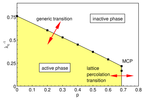
Figure 1: (Color online) Phase diagram of the contact process on a site-diluted cubic lattice (inverse critical infection rate $\lambda_{c}^{-1}$ vs vacancy concentration $p$). MCP marks the multicritical point. The black dots show the actual simulation results, the lines are guides to the eye.

Specifically, there are two different nonequilibrium phase transitions: (i) the so-called generic transition for $p<p_{c}$, driven by the dynamic fluctuations of the contact process and (ii) the lattice percolation transition occurring at $p=p_{c}$ for sufficiently large infection rates Vojta and Lee (2006); Lee and Vojta (2009). The two phase transition lines meet at a multicritical point .

The central quantity of the contact process is the density of infected sites at time $t$,

$$\rho(t)=\frac{1}{L^{d}}\sum_{\mathbf{r}}\langle n_{\mathbf{r}}(t)\rangle~{}.$$ (1)

Here, $n_{\mathbf{r}}(t)$ is the occupation of site $\mathbf{r}$ at time $t$, i.e., $n_{\mathbf{r}}(t)=1$ if the site is infected and $n_{\mathbf{r}}(t)=0$ if it is healthy. $\langle\ldots\rangle$ denotes the average over all realizations of the Markov process. The order parameter of the absorbing-state phase transition is given by the steady state density

$$\rho_{\rm stat}=\lim_{t\to\infty}\rho(t)~{}.$$ (2)

III Scaling theories of absorbing state transitions

In this section, we summarize the scaling theories of the nonequilibrium transitions in the clean and disordered contact process to the extent necessary for analyzing our Monte-Carlo data. We contrast the cases of conventional power-law scaling and activated scaling. More details can be found, for instance, in Ref. Hinrichsen (2000a) for the power-law case and in Refs. Vojta (2006); Igloi and Monthus (2005) for the activated case.

III.1 Conventional critical points

The DP universality class is characterized by three independent critical exponents, for example, $\beta$, $\nu_{\perp}$, and $z$. The order parameter exponent $\beta$ describes how the steady state density varies as the infection rate $\lambda$ approaches its critical value $\lambda_{c}$ from above,

$$\rho_{\rm stat}\sim(\lambda-\lambda_{c})^{\beta}\sim\Delta^{\beta}~{}.$$ (3)

Here, $\Delta=(\lambda-\lambda_{c})/\lambda_{c}$ is the dimensionless distance from criticality. The correlation length exponent $\nu_{\perp}$ describes the divergence of the correlation length $\xi_{\perp}$ at criticality,

$$\xi_{\perp}\sim|\Delta|^{-\nu_{\perp}}~{}.$$ (4)

The correlation time $\xi_{\parallel}$ diverges like a power of the correlation length,

$$\xi_{\parallel}\sim\xi_{\perp}^{z},$$ (5)

which defines the dynamical exponent $z$. In terms of these exponents, the scaling form of the density as a function of $\Delta$, time $t$, and system size $L$ reads

$$\rho(\Delta,t,L)=b^{\beta/\nu_{\perp}}\rho(\Delta b^{-1/\nu_{\perp}},tb^{z},Lb)~{}.$$ (6)

Here, $b$ is an arbitrary dimensionless length scale factor.

If the time evolution starts at time 0 from a single infected site in an otherwise inactive lattice, one can ask what is the probability that an active cluster survives at time $t$. In the DP universality class, this survival probability $P_{s}$ has the same scaling form as the density ,

$$P_{s}(\Delta,t,L)=b^{\beta/\nu_{\perp}}P_{s}(\Delta b^{-1/\nu_{\perp}},tb^{z},Lb)~{}.$$ (7)

The correlation (or pair connectedness) function $C(\mathbf{r},t)=\langle n_{\mathbf{r}}(t)\,n_{0}(0)\rangle$ is given by the probability that site $\mathbf{r}$ is infected at time $t$ when the time evolution starts from a single infected site at $\mathbf{r}=0$ and time $0$. The scale dimension of $C$ is $2\beta/\nu_{\perp}$ because it involves a product of two densities, leading to the scaling form

$$C(\Delta,\mathbf{r},t,L)=b^{2\beta/\nu_{\perp}}C(\Delta b^{-1/\nu_{\perp}},\mathbf{r}b,tb^{z},Lb)~{}.$$ (8)

The total number $N_{s}$ of sites in the active cluster can be calculated by integrating the correlation function over all space, resulting in

$$N_{s}(\Delta,t,L)=b^{2\beta/\nu_{\perp}-d}N_{s}(\Delta b^{-1/\nu_{\perp}},tb^{z},Lb)~{}.$$ (9)

The mean-square radius $R$ of the active cluster has the dimension of a length. Its scaling form therefore reads

$$R(\Delta,t,L)=b^{-1}R(\Delta b^{-1/\nu_{\perp}},tb^{z},Lb)~{}.$$ (10)

The functional dependencies of $\rho$, $P_{s}$, $N_{s}$ and $R$ on the parameters $\Delta$, $t$, and $L$ can be easily derived from the scaling forms by setting the scale factor $b$ to appropriate values. This leads to the following time dependencies at the critical point $\Delta=0$ and in the thermodynamic limit $L\to\infty$. In the long-time limit, the density of infected sites and the survival probability obey the power laws

$$\rho(t)\sim t^{-\delta},\qquad P_{s}(t)\sim t^{-\delta}$$ (11)

with $\delta=\beta/(\nu_{\perp}z)$. The mean-square radius and number of infected sites of a cluster starting from a single seed site behave as

$$R(t)\sim t^{1/z},\qquad N_{s}(t)\sim t^{\Theta}$$ (12)

where $\Theta=d/z-2\beta/(\nu_{\perp}z)$ is the so-called critical initial slip exponent. By taking the derivative of eqs. (6), (7), and (9) with respect to $\Delta$, we also find that

$$\frac{\partial\ln\rho}{\partial\Delta}\sim\frac{\partial\ln P_{s}}{\partial\Delta}\sim\frac{\partial\ln N_{s}}{\partial\Delta}\sim t^{1/(\nu_{\perp}z)}$$ (13)

which will be useful for measuring $\nu_{\perp}$.

III.2 Infinite-randomness critical points

Infinite-randomness critical points feature extremely slow dynamics, represented by an exponential (activated) relation between correlation length and time

$$\ln(\xi_{\parallel}/t_{0})\sim\xi_{\perp}^{\psi},$$ (14)

rather than the power-law dependence (5). It is characterized by the so-called tunneling exponent $\psi$, and $t_{0}$ is a nonuniversal microscopic time scale. The exponential relation between time and length scales implies that the dynamical exponent $z$ is formally infinite. In contrast to the dynamical scaling, the static scaling relations remain of power-law type, i.e., eqs. (3) and (4) remain valid.

The scaling forms of disorder-averaged observables can be obtained by simply substituting the variable combination $\ln(t/t_{0})b^{\psi}$ for $tb^{z}$ in the arguments of the scaling functions:

$$\rho(\Delta,\ln(t/t_{0}),L)=b^{\beta/\nu_{\perp}}\rho(\Delta b^{-1/\nu_{\perp}},\ln(t/t_{0})b^{\psi},Lb)~{},$$ (15)

$$P_{s}(\Delta,\ln(t/t_{0}),L)=b^{\beta/\nu_{\perp}}P_{s}(\Delta b^{-1/\nu_{\perp}},\ln(t/t_{0})b^{\psi},Lb)~{},$$ (16)

$$N(\Delta,\ln(t/t_{0}),L)=b^{2\beta/\nu_{\perp}-d}N(\Delta b^{-1/\nu_{\perp}},\ln(t/t_{0})b^{\psi},Lb)~{},$$ (17)

$$R(\Delta,\ln(t/t_{0}),L)=b^{-1}R(\Delta b^{-1/\nu_{\perp}},\ln(t/t_{0})b^{\psi},Lb)~{}.$$ (18)

Consequently, the critical time dependencies of the density of active sites and the survival probability (in the thermodynamic limit) are logarithmic,

$$\rho(t)\sim[\ln(t/t_{0})]^{-\bar{\delta}},\qquad P_{s}(t)\sim[\ln(t/t_{0})]^{-\bar{\delta}}$$ (19)

with $\bar{\delta}=\beta/(\nu_{\perp}\psi)$. The radius and number of active sites in a cluster starting from a single seed site vary as

$$R(t)\sim[\ln(t/t_{0})]^{1/\psi},\qquad N_{s}(t)\sim[\ln(t/t_{0})]^{\bar{\Theta}}$$ (20)

with $\bar{\Theta}=d/\psi-2\beta/(\nu_{\perp}\psi)$. Taking the derivatives of eqs. (15), (16), and (17) with respect to $\Delta$ yields

$$\frac{\partial\ln\rho}{\partial\Delta}\sim\frac{\partial\ln P_{s}}{\partial\Delta}\sim\frac{\partial\ln N_{s}}{\partial\Delta}\sim[\ln(t/t_{0})]^{1/(\nu_{\perp}\psi)}~{}.$$ (21)

III.3 Griffiths region

In the presence of spatial disorder, the contact process displays unconventional behavior not just at the critical point but also in its vicinity because rare active spatial regions dominate the long-time dynamics. This phenomenon is an example of the well-known Griffiths singularities Griffiths (1969) that generally occur at phase transitions in disordered systems (see Ref. Vojta (2006) for a review). The Griffiths singularities in the spatially disordered contact process can be understood as follows Noest (1986).

The inactive phase must be divided into two regions. (i) If the infection rate is below the clean critical value, $\lambda<\lambda_{c}^{0}$, the behavior is conventional. This means, the system approaches the absorbing state exponentially fast. The decay time increases with $\lambda$ and diverges as $|\lambda-\lambda_{c}^{0}|^{-z\nu_{\perp}}$ where $z$ and $\nu_{\perp}$ are the exponents of the clean critical point Vojta and Dickison (2005); Dickison and Vojta (2005).

(ii) If the infection rate is in the so-called Griffiths region (or Griffiths phase) between the clean and dirty critical values, $\lambda_{c}^{0}<\lambda<\lambda_{c}$, the system is globally still in the inactive phase (i.e., it eventually decays into the absorbing state). However, in the thermodynamic limit, one can find arbitrarily large spatial regions devoid of vacancies. These rare regions are locally in the active phase. Although they cannot support a non-zero steady state density because they are of finite size, their time decay is very slow as it requires a rare, exceptionally large density fluctuation.

The contribution of the rare regions to the density of infected sites can be expressed as the integral

$$\rho(t)\sim\int dL_{r}~{}L_{r}^{d}~{}w(L_{r})\exp\left[-t/\tau(L_{r})\right]~{}.$$ (22)

Here, $w$ denotes the probability for finding a spatial region of size $L_{r}$ that does not contain any vacancies, and $\tau(L_{r})$ is the life time of the contact process on such a rare region. Basic combinatorics gives

$$w(L_{r})\sim\exp(-\tilde{p}L_{r}^{d})$$ (23)

with $\tilde{p}=-\ln(1-p)$ (up to pre-exponential factors). In the Griffiths phase, the life time of a rare region depends exponentially on its volume,

$$\tau(L_{r})\sim\exp(aL_{r}^{d})$$ (24)

because a coordinated fluctuation of the entire region is necessary to take it to the absorbing state Noest (1986, 1988); Schonmann (1985). The constant $a$ vanishes at the clean critical infection rate $\lambda_{c}^{0}$ and increases with $\lambda$. Evaluating the integral (22) in saddle-point approximation, we obtain a power-law time dependence for the density. The survival probability $P_{s}$ shows exactly the same time dependence,

$$\rho(t)\sim P_{s}(t)\sim t^{-\tilde{p}/a}=t^{-d/z^{\prime}}~{},$$ (25)

where $z^{\prime}=da/\tilde{p}$ is the nonuniversal dynamical exponent in the Griffiths region. The behavior of $z^{\prime}$ close to the dirty critical point can be obtained from the SDRG analysis Hooyberghs et al. (2004); Fisher (1995); Motrunich et al. (2000). As $\lambda$ approaches $\lambda_{c}$, $z^{\prime}$ diverges as

$$z^{\prime}\sim|\lambda-\lambda_{c}|^{-\psi\nu_{\perp}}$$ (26)

where $\psi$ and $\nu_{\perp}$ are the critical exponents of the infinite-randomness critical point.

IV Monte-Carlo simulations

IV.1 Simulation method

To perform Monte Carlo simulations of the contact process on randomly diluted cubic lattices, we followed the implementation described, for instance, by Dickman Dickman (1999). The algorithm starts at time $t=0$ from some configuration of infected and healthy sites and consists of a sequence of events. During each event an infected site is randomly chosen from a list of all $N_{a}$ infected sites, then a process is selected, either infection of a neighbor with probability $\lambda/(1+\lambda)$ or healing with probability $1/(1+\lambda)$. For infection, one of the six neighbor sites is chosen at random. The infection succeeds if this neighbor is healthy (and not a vacancy site). The time is then incremented by $1/N_{a}$.

Using this algorithm, we simulated systems with sizes of up to $999^{3}$ sites and vacancy concentrations $p=0$, 0.2, 0.3, 0.4, 0.5, 0.6 and $p_{c}=0.6883920$ Lorenz and Ziff (1998). To cope with the slow dynamics of the disordered contact process, we simulated long times up to $10^{8}$. All results were averaged over a large number of disorder configurations, precise numbers will be given below.

We carried out two different types of simulations. (i) The majority of runs started from a single active site in an otherwise inactive lattice (spreading runs); we monitored the survival probability $P_{s}(t)$, the number of sites $N_{s}(t)$ of the active cluster, and its radius $R(t)$. (ii) For comparison, we also performed a few runs that started from a completely active lattice during which we observed the time evolution of the density $\rho(t)$.

We employed two different high-quality, long-period random number generators. Most simulations used LFSR113 proposed by L’Ecuyer L’Ecuyer (1999). We verified the validity of the results by means of the 2005 version of Marsaglia’s KISS Marsaglia (2005). The total computational effort for the work described in this paper was about 100 000 CPU days on the Pegasus cluster at Missouri S&T.

Figure 1 gives an overview of the phase diagram resulting from these simulations. As expected, the critical infection rate $\lambda_{c}$ increases with increasing impurity concentration.

IV.2 Contact process on an undiluted lattice

The purpose of studying the clean three-dimensional contact process is two-fold, (i) to test our implementation of the contact process and (ii) to compute highly accurate estimates of the critical exponents in the three-dimensional DP universality class. To reduce the numerical effort, we applied the clever reweighting technique proposed in Ref. Dickman (1999).

After a few test calculations aimed at bracketing the critical point, we performed two large spreading runs (starting from a single active site) at $\lambda=1.3168400$. By reweighting with a step $\Delta\lambda=0.0000025$, we generated data for $\lambda$ between 1.3168150 and 1.3168650. The first run consisted of $4\times 10^{8}$ trials using the LFSR113 random number generator, the second consisted of $5\times 10^{8}$ trials using the KISS random number generator. The maximum time of both runs was $5\times 10^{4}$. As the data of both runs agree within their statistical error, we averaged their results. The system size, $850^{3}$ sites, was chosen such that the active cluster stayed smaller than the sample during the entire time evolution, eliminating finite-size effects.

To find the location of the critical point and to measure the critical exponents, we define effective (running) exponents via the logarithmic derivatives of various observables. These effective exponents are then extrapolated to $t=\infty$. The finite-size scaling exponent $\beta/\nu_{\perp}$ (scale dimension of the order parameter) can be determined from the relation between $N_{s}$ and $P_{s}$. Combining (11) and (12) yields $N_{s}\sim P_{s}^{-\Theta/\delta}$ with $\Theta/\delta=3\nu_{\perp}/\beta-2$. Figure 2 shows the effective exponent $(d\ln N_{s})/(d\ln P_{s})$ as a function of $t^{-y}$ with $y=1/2$.

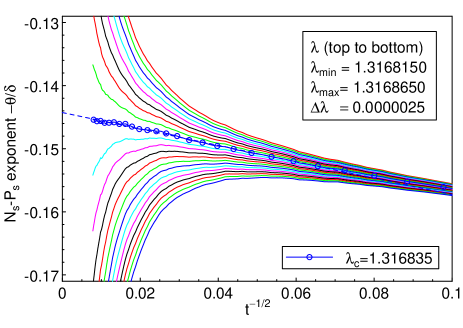
Figure 2: (Color online) Effective critical exponent $-\Theta/\delta=(d\ln N_{s})/(d\ln P_{s})$ vs. $t^{-1/2}$. The critical curve is marked by dots, and the dashed line is a linear extrapolation to $t=\infty$.

(The value 1/2 was chosen empirically to allow a linear extrapolation to $t=\infty$.) From this plot, we estimate the critical infection rate to be

$$\lambda_{c}^{0}=1.316835(1)~{}.$$ (27)

We verified this value by performing an extra run directly at $\lambda=1.316835$ using $4\times 10^{8}$ trials on a system of size $999^{3}$ with a maximum time of $10^{5}$.

Extrapolating the effective exponent to $t=\infty$, we obtain $\Theta/\delta=0.1442(3)_{\rm sys}(2)_{\rm ran}$ where the values in brackets represent estimates of the systematic and random errors of the last digit. The systematic error stems from the uncertainties of $\lambda_{c}^{0}$ and the extrapolation exponent $y$ while the random error is due to the Monte-Carlo noise. The resulting value of the finite-size scaling exponent is $\beta/\nu_{\perp}=1.3991(4)$. An estimate for this exponent can also be obtained from the relation between $N_{s}$ and $R$. Extrapolating the effective exponent as above yields the identical value $\beta/\nu_{\perp}=1.3991(4)$.

To determine the exponents $z$, $\delta$, and $\Theta$, we apply the same type of analysis to the logarithmic derivatives of $R$, $P_{s}$, and $N_{s}$ with respect to time. The corresponding graphs are shown in Fig. 3.

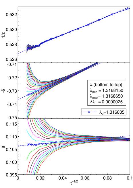
Figure 3: (Color online) Effective critical exponents $1/z=(d\ln R)/(d\ln t)$, $\delta=(d\ln P_{s})/(d\ln t)$ and $\Theta=(d\ln N_{s})/(d\ln t)$ vs. $t^{-1/2}$. The critical curves are marked by dots, and the dashed lines are linear extrapolations to $t=\infty$.

Extrapolation to $t=\infty$ yields the dynamical exponent $1/z=0.5267(1)_{\rm sys}(1)_{\rm ran}$ as well as $\delta=0.7367(5)_{\rm sys}(1)_{\rm ran}$ and $\Theta=0.1062(2)_{\rm sys}(2)_{\rm ran}$. These values fulfill hyperscaling because $\Theta+2\delta-3/z=-0.0005(22)$, in excellent agreement with the exact result of zero.

Finally, we measure the exponent combination $1/(\nu_{\perp}z)$ by analyzing the time dependencies of $({\partial\ln P_{s}})/({\partial\lambda})$ and $({\partial\ln N_{s}})/({\partial\lambda})$ according to (13). Extrapolating the effective exponent to $t=\infty$ as above yields $1/(\nu_{\perp}z)=0.9040(5)_{\rm sys}(5)_{\rm ran}$. The correlation length and order parameter exponents can be calculated by combining this value with our results for $z$ and $\beta/\nu_{\perp}$ yielding $\nu_{\perp}=0.5826(9)$ and $\beta=0.815(2)$.

In Table 1, we compare our estimates for the critical exponents with earlier results.

Value	This work	Ref. Sander et al. (2009)	Ref. Dickman (1999)	Ref. Sabag and de Oliveira (2002)	Ref. Jensen (1992)
$\lambda_{c}^{0}$	1.316835(1)	(*)	1.31686(1)	1.31683(2)	1.3168(1)
$\beta/\nu_{\perp}$	1.3991(4)	1.395(4)	1.394(1)		1.392(5)
$\nu_{\perp}$	0.5826(9)		0.580(3)		0.584(6)
$\beta$	0.815(2)		0.808(5)	0.78(1)	0.813(11)
$\delta$	0.7367(6)		0.7263(11)		0.732(4)
$\Theta$	0.1062(4)		0.110(1)		0.114(4)
$z$	1.8986(8)	1.916(5)	1.919(4)		1.901(5)
$2/z$	1.0534(4)		1.042(2)		1.052(3)
$\nu_{\perp}z$	1.106(2)		1.114(4)		1.11(1)
$\Theta z$	0.2016(6)	0.216(3)
$D_{f}$	1.6009(4)			1.56(3)

Table 1: Critical infection rate and critical exponents of the clean three-dimensional contact process. The upright numbers are directly given in the respective papers, the italic ones were calculated using scaling relations. The fractal dimension $D_{f}=3-\beta/\nu_{\perp}$. (*) The authors of Ref. Sander et al. (2009) used the value of $\lambda_{c}$ found in Ref. Dickman (1999) as an input.

The present estimates have significantly higher precision than the values in the literature. They are roughly compatible with Jensen’s values Jensen (1992) within their given errors (for $\Theta$, the difference is about twice the given error, though). However, they are clearly not compatible with the values given in Refs. Dickman (1999) and Sander et al. (2009) (for $\delta$, the difference is about ten times the given error, and for $z$ it is about five times the given error). We believe, this discrepancy can be traced back to the location of the critical point. According to our data, the infection rate $\lambda=1.31686(1)$, identified as critical in Ref.  Dickman (1999) and also employed in Sander et al. (2009), is on the active side of the transition (it differs from our estimate by about three times the given error). As the survival probability decays more slowly in the active phase than at criticality, this may be responsible for the low $\delta$-value and, via the hyperscaling relation, for the high $z$-value reported in Ref. Dickman (1999).

IV.3 Contact process on a diluted lattice

The remainder of Sec. IV focuses on the contact process on a diluted lattice. We tried to use the same reweighting technique as in the clean case to save computer time. However, these attempts were not successful. The reweighing method of Ref. Dickman (1999) considers a set of simulation runs (particular realizations of the Markov process) at some infection rate $\lambda$ and reweighs their statistical probabilities according to a slightly different $\lambda^{\prime}$. This only works as long as the two infection rates are sufficiently close such that their sets of possible runs overlap significantly. This overlap decreases with increasing simulation time. In the presence of disorder, particularly long simulation times are required because the critical dynamics is logarithmically slow. Thus, reweighting is restricted to very narrow $\lambda$-intervals (too narrow compared to the range of infection rates we needed to explore to determine the critical point). All results were thus obtained in the conventional manner by performing a separate run for each $\lambda$-value.

Figure 4 gives an overview over spreading simulations (starting from a single active seed site) for a vacancy concentration $p=0.5$.

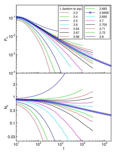
Figure 4: (Color online) Survival probability $P_{s}$ and number of active sites $N_{s}$ vs. time $t$ for impurity concentration $p=0.5$ and several infection rates $\lambda$. The critical curve at $\lambda_{c}=2.6906$ is marked by dots.

The data represent averages over at least 5000 disorder configurations, with 128 trials starting from random seed sites for each configuration. A system size of $500^{3}$ sites ensured that the active cluster stayed smaller than the sample for the entire simulation run. The figure shows that the dynamics in the vicinity of the phase transition is very slow. In particular, the time-dependence of the survival probability appears to be slower than a power law, in agreement with the activated scaling scenario of Sec. III.2. Moreover, the data show indications of Griffiths singularities, i.e., nonuniversal power-law behavior somewhat below the critical infection rate. We also note that the number of sites in the active cluster $N_{s}$ decreases with time at the transition, in contrast to the clean case and to the diluted case in two dimensions Vojta et al. (2009). This implies a negative exponent $\bar{\Theta}$.

To find the precise location of the critical point within the activated scaling scenario, one might be tempted to search for power-law relations between $\ln t$ and observables such $P_{s}$ and $N_{s}$ (either by plotting $\ln P_{s}$ and $\ln N_{s}$ vs. $\ln\ln t$ or by analyzing the corresponding effective exponents). However, this method is highly unreliable as the unknown microscopic time scale $t_{0}$ in (19) and (20) provides a correction to scaling via $\ln(t/t_{0})=\ln t-\ln t_{0}$. This strongly influences the results because the simulations cover only a moderate range in $\ln t$. (In the two-dimensional simulations, Ref. Vojta et al. (2009), it was found that neglecting $t_{0}$ could change the apparent value of $\bar{\delta}$ from its correct value of 1.9 to 3.)

To circumvent this problem, we follow the method devised in Ref. Vojta et al. (2009). It is based on the observation that $t_{0}$ has the same value in the scaling forms of all quantities because it is related to the energy scale $\Omega_{0}$ of the underlying SDRG. Consequently, if one analyzes the relation between $N_{s}$ and $P_{s}$ or other such combinations of observables, the critical point corresponds to power-law behavior (independent of the value of $t_{0}$) as long as all other corrections to scaling are small.

We performed long spreading runs with a maximum time of $5\times 10^{7}$, system size $500^{3}$ and vacancy concentration $p=0.5$ for several infection rates $\lambda$ close to the phase transition. The resulting plot of $N_{s}$ vs $P_{s}$ is shown in Figure 5.

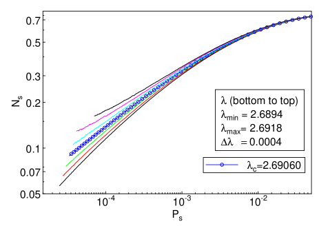
Figure 5: (Color online) $N_{s}$ versus $P_{s}$ for vacancy concentration $p=0.5$ and several infection rates $\lambda$ close to the critical point.

The data are averages over $10^{5}$ to $10^{6}$ disorder configurations with 1000 trials starting from random seed sites for each configuration. The figure shows that the relation between $N_{s}$ and $P_{s}$ indeed approaches a power law in the long-time (small $P_{s}$) limit. The figure also indicates that the crossover to the asymptotic behavior is very slow. The asymptotic power law is only reached when $P_{s}$ falls well below $10^{-3}$ which corresponds to times larger than $10^{4}$, implying that long simulations are required to determine the critical behavior. Moreover, the mean-square radius of the active cluster at the crossover time is approximately 25, implying a total diameter of about 100. This means that simulations of systems with less than $100^{3}$ sites will never reach the asymptotic critical behavior.

IV.4 Critical exponents

To find the critical infection rate $\lambda_{c}$ and to measure the finite-size scaling exponent $\beta/\nu_{\perp}$ (the scale dimension of the order parameter), we define the effective (running) exponent $(d\ln N_{s})/(d\ln P_{s})=-\bar{\Theta}/\bar{\delta}$. It is related to the finite-size scaling exponent via $\bar{\Theta}/\bar{\delta}=3\nu_{\perp}/\beta-2$ [see eqs. (19) and (20)]. To avoid the uncertainties stemming from the unknown microscopic time scale $t_{0}$, we extrapolate this effective exponent to $P_{s}=0$ rather than $t=\infty$. Figure 6 shows the effective exponent as a function of $P_{s}^{\bar{y}}$ with $\bar{y}=1/2$.

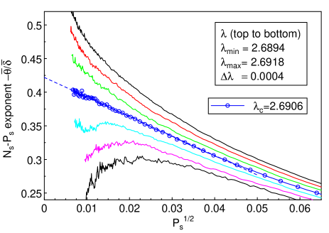
Figure 6: (Color online) Effective critical exponent $-\bar{\Theta}/\bar{\delta}=(d\ln N_{s})/(d\ln P_{s})$ vs. $P_{s}^{1/2}$ calculated from the data in Fig. 5. The critical curve is marked by dots, and the dashed line is a linear extrapolation to $P_{s}=0$.

(The value 1/2 was again chosen empirically to permit an approximately linear extrapolation of the data with $P_{s}\lesssim 10^{-3}$. Because of the slow crossover to the asymptotic regime, the value of $\bar{y}$ is much more uncertain than that of $y$ in the clean case, see Fig. 2.)

From Fig. 6, we conclude that $\lambda_{c}=2.6906(3)$ for a vacancy concentration of $p=0.5$. Extrapolating the effective exponent to $P_{s}=0$ yields $\bar{\Theta}/\bar{\delta}=-0.42(3)$ where the error estimate largely stems from the uncertainty in $\lambda_{c}$ (and the related uncertainty in $\bar{y}$.) The statistical error is much smaller. The resulting finite-size scaling exponent is $\beta/\nu_{\perp}=1.90(4)$. An estimate for this exponent can also be obtained from analyzing the dependence of $N_{s}$ on $R$ in a similar fashion. The data show additional curvature (corrections to scaling), thus giving the less precise value $\beta/\nu_{\perp}=1.85(15)$.

We now apply the same type of analysis to the logarithmic derivatives of $P_{s}$, $N_{s}$, and $R$ with respect to $\ln(t/t_{0})$ to determine the values of the exponents $\bar{\delta}$, $\bar{\Theta}$, and $\psi$. This requires a value for the microscopic time scale $t_{0}$. Since an incorrect $t_{0}$ would produce additional corrections to scaling, we estimated its value by minimizing the time dependence ($P_{s}$ dependence) of the effective exponents $\bar{\delta}$ and $\bar{\Theta}$. This yields $t_{0}\approx 1.0(4)$. Figure 7 shows the resulting effective exponents $\bar{\delta}$ and $\bar{\Theta}$ as a function of $P_{s}^{1/2}$ for vacancy concentration $p=0.5$.

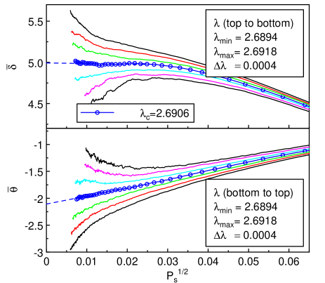
Figure 7: (Color online) Effective critical exponents $\bar{\delta}=-(d\ln P_{s})/(d\ln\ln(t/t_{0}))$ and $\bar{\Theta}=(d\ln N_{s})/(d\ln\ln(t/t_{0}))$ vs. $P_{s}^{1/2}$ for $p=0.5$ and $t_{0}=1$. The critical curves are marked by dots, and the dashed lines are linear extrapolations to $P_{s}=0$.

Extrapolating the data at the critical infection rate $\lambda_{c}=2.6906$ to $P_{s}=0$ (i.e., $t=\infty$) gives the values $\bar{\delta}=5.0(2)$ and $\bar{\Theta}=-2.1(2)$. Again, the error estimate is dominated by the uncertainty in $\lambda_{c}$ (and the resulting uncertainties in $\bar{y}$ and $t_{0}$). The tunneling exponent $\psi$ can be determined by combining the value of $\beta/\nu_{\perp}$ with either $\bar{\delta}$ or $\bar{\Theta}$. We find $\psi=0.38(3)$. Alternatively, $\psi$ can be obtained from the dependence of $R$ on $\ln(t/t_{0})$. As these data show additional corrections to scaling, the extrapolation to $t=\infty$ is difficult and leads to the less precise estimate $\psi=0.41(5)$.

To find the critical exponents $\nu_{\perp}$ and $\beta$, we now study the dependence of $({\partial\ln P_{s}})/({\partial\lambda})$ and $({\partial\ln N_{s}})/({\partial\lambda})$ on $\ln(t/t_{0})$ according to eq. (21). This yields the exponent combination $1/\nu_{\perp}\psi=2.7(3)$. Combining this with the value for $\psi$, we obtain $\nu_{\perp}=1.0(2)$. This analysis is hampered by the rather large uncertainties in $\psi$ and $t_{0}$. A better estimate can be obtained by considering the dependence of $({\partial\ln P_{s}})/({\partial\lambda})$ and $({\partial\ln N_{s}})/({\partial\lambda})$ on $P_{s}$ which takes the form

$$\frac{\partial\ln P_{s}}{\partial\lambda}\sim\frac{\partial\ln N_{s}}{\partial\lambda}\sim P_{s}^{-1/\beta}~{}.$$ (28)

Extrapolating the effective exponents to $P_{s}=0$ as before, we obtain the values $1/\beta$ =0.53(2) and 0.55(3) from the $P_{s}$ and $N_{s}$ data, respectively. Our final estimate of the order parameter exponent is thus $\beta=1.87(7)$. Combined with the finite-size scaling exponent, this yields $\nu_{\perp}=0.98(6)$.

In Table 2, we compare our estimates for the critical exponents with results of a numerical SDRG calculation Kovács and Iglói (2011) of the random transverse-field Ising model with up to $128^{3}$ sites. This model is expected to be in the same universality class as the disordered contact process.

Value	This work	Ref. Kovács and Iglói (2011)
$\beta/\nu_{\perp}$	1.90(4)	1.84(2)
$\nu_{\perp}$	0.98(6)	0.99(2)
$\beta$	1.87(7)	1.82(4)
$D_{f}$	1.10(4)	1.16(2)
$\psi$	0.38(3)	0.46(2)
$\nu_{\perp}\psi$	0.37(4)	0.45(3)
$\bar{\delta}$	5.0(2)	4.0(2)
$\bar{\Theta}$	-2.1(2)	-1.5(1)

Table 2: Critical exponents of the disordered three-dimensional contact process compared to results of the SDRG calculation Kovács and Iglói (2011). The upright numbers are directly given in Ref. Kovács and Iglói (2011), the italic ones were calculated using scaling relations. The fractal dimension $D_{f}=3-\beta/\nu_{\perp}$.

All static exponents (above the dividing line in the table) agree within their error bars (though just barely in the case of $\beta/\nu_{\perp}$). In contrast, the tunneling exponent $\psi$ and the other exponents characterizing the time dependencies (below the dividing line) do not agree. This suggests that the uncertainties in determining the microscopic time scale $t_{0}$ and, correspondingly, the microscopic energy scale $\Omega_{0}$ of the SDRG calculation may be responsible for the disagreement because $t_{0}$ and $\Omega_{0}$ do not influence the static exponents. We note, however, that our raw data do not seem to be compatible with the values for $\bar{\delta}$ and $\bar{\Theta}$ calculated from the results of Ref. Kovács and Iglói (2011) even if we allow $t_{0}$ to vary (unless one assumes a crossover from our $\bar{\delta}=5$ to $\bar{\delta}=4$ and from $\bar{\Theta}=2$ to $\bar{\Theta}=1.5$ at times $t\gtrsim 10^{8}$ beyond the range of our simulations). This can be seen in Fig. 8 where we compare our data to the functions $P_{s}\sim\ln(t/t_{0})^{-4}$ and $N_{s}\sim\ln(t/t_{0})^{-1.5}$ with $\ln(t_{0})$ = 0, 1, 2, 3, and 4.

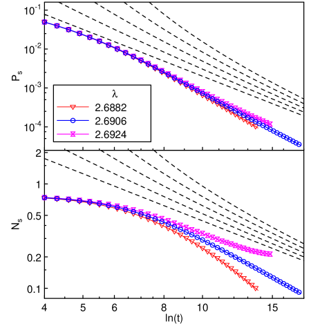
Figure 8: (Color online) Time dependence of $P_{s}$ and $N_{s}$ for impurity concentration $p=0.5$ and several $\lambda$ close to the transition compared to the predictions of the numerical SDRG of Ref. Kovács and Iglói (2011). The dashed lines represent the functions $P_{s}\sim\ln(t/t_{0})^{-4}$ and $N_{s}\sim\ln(t/t_{0})^{-1.5}$ with $\ln(t_{0})$ = 0, 1, 2, 3, 4 (bottom to top) and arbitrary prefactor.

We will return to this question in the concluding section.

IV.5 Universality of the critical behavior

So far, all results on the disordered contact process were for a vacancy concentration $p=0.5$. We now address the question of whether or not the critical behavior is universal, i.e., independent of the disorder strength. The SDRG underlying the infinite-randomness scenario becomes exact only for infinitely strong disorder (infinitely broad disorder distributions). Therefore, it cannot decide the fate of a weakly disordered system. However, Janssen’s perturbative renormalization group Janssen (1997), which is controlled for weak disorder, shows runaway flow towards large disorder strength. Furthermore, Hoyos Hoyos (2008) showed that within an improved SDRG scheme, the disorder always increases under renormalization, even if it is weak initially. These arguments support a universal scenario in which the critical behavior is independent of the disorder strength.

To study the question of universality numerically, we performed simulations for vacancy concentrations $p=0.2$, 0.3, 0.4, and 0.6 in addition to the value 0.5. Repeating the complete analysis as discussed in the previous subsections for all values of $p$ would have been prohibitively expensive in terms of computer time. We therefore focused on finding the finite-size scaling exponent from $N_{s}$ vs. $P_{s}$ plots analogously to Fig. 5, using somewhat shorter runs. The maximum time was at least $3\times 10^{6}$ for all vacancy concentrations, and the data are averages over at least $10^{7}$ trials using systems of $500^{3}$ or $720^{3}$ sites. The resulting critical curves are presented in the upper panel of Fig. 9.

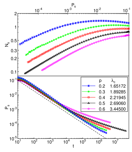
Figure 9: (Color online) Upper panel: $N_{s}$ vs. $P_{s}$ at criticality for several vacancy concentrations $p$. Lower panel: $P_{s}$ vs. $t$ at criticality, demonstrating the crossover from the clean to the dirty critical behavior. The dashed line represents a power law with the clean critical exponent $\delta=0.7366$ and arbitrary prefactor.

In the low-$P_{s}$ (long-time) limit, all curves appear to be parallel, implying that $\bar{\Theta}/\bar{\delta}$ and with it the finite-size scaling exponent $\beta/\nu_{\perp}$ takes the same value for all vacancy concentrations. The figure also suggests that the weak-disorder curves (in particular $p=0.2$) have not fully crossed over to the asymptotic critical behavior. This is confirmed in the lower panel of Fig. 9 which presents a log-log plot of $P_{s}$ vs. $t$ at criticality. While the stronger-disorder curves ($p=0.5$, 0.6) start to deviate from the clean critical power law at $t\approx 10^{3}$ to $10^{4}$ (in agreement with the estimate discussed at the end of Sec. IV.3), the $p=0.2$ curve deviates appreciably only after $t\approx 10^{6}$. (Note that these long crossover times also imply huge system sizes to reach the asymptotic regime. For $p=0.2$, the mean-square radius of the active cloud at the crossover time of $10^{6}$ is about 200.)

Our simulations thus show no indications of nonuniversal, continuously varying critical exponents. However, we cannot rigorously exclude that the exponents change for very weak disorder, because the extremely large crossover times between the clean and the dirty critical behavior prevent us from reaching the asymptotic regime in these cases.

IV.6 Griffiths region

In order to investigate the Griffiths region $\lambda_{c}^{0}<\lambda<\lambda_{c}$, we have also performed detailed simulations for infection rates $\lambda$ below but close to the critical rate $\lambda_{c}$. Figure 10 presents the resulting survival probability $P_{s}$ as a function of time $t$ for vacancy concentration $p=0.5$.

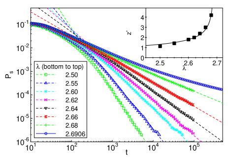
Figure 10: (Color online) $P_{s}$ vs. $t$ for several infection rates $\lambda$ in the Griffiths region $\lambda_{c}^{0}<\lambda<\lambda_{c}$ (vacancy concentration $p=0.5$). The dashed lines are power-law fits of the long-time behavior to (25). Inset: Resulting Griffiths dynamical exponent $z^{\prime}$ as a function of $\lambda$. The solid line is a fit to (26).

The data are averages over at least 10000 disorder configurations with 1000 trials per configuration. The system size is $300^{3}$ sites. For all infection rates shown, the long-time decay of the survival probability obeys (over several orders of magnitude in $P_{s}$ and/or $t$) the nonuniversal power law predicted by the rare region arguments of Sec. III.3.

The Griffiths dynamical exponent $z^{\prime}$ can be found by fitting the long-time decay to (25). The resulting values, shown in the inset of Fig. 10, demonstrate that $z^{\prime}$ diverges as $\lambda$ approaches the critical value $\lambda_{c}=2.6906$. Fitting $z^{\prime}$ to the expected power law (26) gives a value for the combination $\nu_{\perp}\psi$. The fit is not of particularly high quality, but the resulting value, $\nu_{\perp}\psi=0.42(6)$, is in reasonable agreement with the value determined at criticality.

IV.7 Contact process at the lattice percolation threshold

This subsection is devoted to the nonequilibrium phase transition of the diluted contact process across the lattice percolation threshold $p_{c}$. In the phase diagram shown in Fig. 1, this transition is marked by the vertical line at $p_{c}$ between $\lambda_{c}^{-1}=0$ and the multicritical point.

The contact process on a diluted lattice close to the percolation threshold can be understood by combining classical percolation theory with the properties of the supercritical contact process on finite-size clusters Vojta and Lee (2006); Lee and Vojta (2009). Although its behavior follows the activated scaling scenario described in subsection III.2, the critical exponents of the percolation transition differ from those of the generic transition discussed in the preceding sections. Interestingly, they are completely determined by the values of the classical lattice percolation exponents $\beta_{c}$ and $\nu_{c}$ which are known numerically with high accuracy Stauffer and Aharony (1991).

According to Refs.  Vojta and Lee (2006); Lee and Vojta (2009), the order parameter exponent $\beta$ and the correlation length exponent $\nu_{\perp}$ of the nonequilibrium phase transition are identical to the corresponding lattice exponents, $\beta=\beta_{c}=0.417$ and $\nu_{\perp}=\nu_{c}=0.875$. The tunneling exponent $\psi$ is given by the fractal dimension $D_{c}$ of the critical lattice percolation cluster, $\psi=D_{c}=3-\beta_{c}/\nu_{c}=2.523$. As a result, the critical exponent $\bar{\delta}$ takes a very small value, $\bar{\delta}=\beta/(\nu_{\perp}\psi)=0.188$.

We performed spreading simulation runs (starting from a single active site) at $p_{c}=0.6883920$ Lorenz and Ziff (1998) and $\lambda=6.0$ to a maximum time of $5\times 10^{5}$. Because of the small value of $\bar{\delta}$, these simulations are particularly time consuming. The resulting survival probability $P_{s}$ (averaged over 230 disorder configurations with 200 trials per configuration) is presented in Fig. 11.

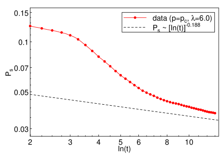
Figure 11: (Color online) $P_{s}$ vs $\ln(t)$ for $p=p_{c}=0.6883920$ and $\lambda=6.0$. The dashed line represents the expected logarithmic long-time decay, $P_{s}\sim[\ln(t)]^{-\bar{\delta}}$ with $\bar{\delta}=0.188$ and arbitrary prefactor.

The data are in agreement with the qualitative predictions of Refs. Vojta and Lee (2006); Lee and Vojta (2009): a rapid initial decay towards a quasi-stationary state, followed by a slow logarithmic time dependence due to the successive dying out of the contact process on larger and larger lattice percolation clusters. The figure shows that the long-time behavior of our data is compatible with the predicted exponent value $\bar{\delta}=0.188$. However, we found it impossible to calculate a precise value of $\bar{\delta}$ directly from the simulation data because the long-time decay is extremely slow.

V Summary and conclusions

To summarize, we performed large-scale Monte Carlo simulations of the contact process on site-diluted cubic lattices. We determined the infection rate–dilution phase diagram. It features two different nonequilibrium phase transitions, (i) the generic transition that occurs for dilutions below the percolation threshold of the lattice and is driven by the dynamic fluctuations of the contact process, and (ii) the transition across the percolation threshold which is driven by the lattice geometry.

Our simulation results show that the generic transition is controlled by an infinite-randomness critical point for all dilutions investigated. It gives rise to ultraslow activated (exponential) dynamical scaling instead of the power-law dynamical scaling at conventional critical points. The corresponding logarithmic time dependencies of various observables at criticality required long simulation times and thus a huge numerical effort (in total about 100 000 CPU days on the Pegasus cluster at Missouri S&T). We determined the complete critical behavior of the generic transition and found it to be universal, i.e., independent of the disorder strength (dilution).

The critical exponents are listed in Table 2, together with results of a numerical SDRG calculation Kovács and Iglói (2011) of the three-dimensional random transverse-field Ising model which is predicted to be in the same universality class. We were able to calculate reasonably accurate estimates for the static critical exponents including the finite-size scaling exponent $\beta/\nu_{\perp}$, the order-parameter exponent $\beta$ and the spatial correlation length exponent $\nu_{\perp}$. The correlation length exponent satisfies the inequality $d\nu_{\perp}>2$, as is expected in a disordered system Chayes et al. (1986). Our values for the static exponents agree with the corresponding numerical SDRG results of Ref. Kovács and Iglói (2011) within the given errors. In contrast, our result for the tunneling exponent $\psi$ as well as $\bar{\delta}$ and $\bar{\Theta}$ do not agree with the values quoted in Ref. Kovács and Iglói (2011). Estimates of $\psi$, $\bar{\delta}$ and $\bar{\Theta}$ depend sensitively on the microscopic time scale $t_{0}$ or, correspondingly, on the microscopic energy scale $\Omega_{0}$ in the numerical SDRG calculation, while the static exponents are independent of it. This suggests that uncertainties in the value of $t_{0}$ or $\Omega_{0}$ may be responsible for the disagreement. However, even if we allow the value of $t_{0}$ to vary, our $P_{s}$ and $N_{s}$ data do not seem to be compatible with the values of $\bar{\delta}$ and $\bar{\Theta}$ predicted by Ref. Kovács and Iglói (2011).

The differences between our results and the numerical SDRG calculation could either imply a real difference in universality class, or they could mean that one or both sets of results represent effective rather than true asymptotic exponents. A full resolution of this question will likely require much more extensive simulations together with a careful analysis of finite-size effects and, in particular, of the microscopic time/energy scale in the infinite-randomness scenario.

In addition to the generic transition, we briefly studied the nonequilibrium transition across the lattice percolation threshold. The Monte Carlo results support the predictions of the theory developed in Refs. Vojta and Lee (2006); Lee and Vojta (2009): The dynamical critical behavior is of activated type with critical exponents that are combinations of the classical lattice percolation exponents. Our simulations also allowed us to find with reasonable accuracy the location of the multicritical point separating the generic transition from the percolation transition (see Fig. 1). However, as the dynamics is expected to be even slower than that of the generic transition, finding the true multicritical behavior appears to be beyond our current computational resources.

We also obtained high-precision estimates for the critical behavior of the three-dimensional DP universality class by performing simulations of the clean contact process in three dimensions. We employed the reweighting technique proposed by Dickman Dickman (1999) to save computer time. By using large lattices of up to $999^{3}$ sites and long times of up to $5\times 10^{4}$, we were able to compute the critical exponents with unprecedented accuracy (see Table 1). As the dynamics of the clean contact process is much faster than that of the disordered contact process, this part of the work took only a small fraction (about 5000 CPU days) of the overall computer time.

Let us now put our results into broader perspective. Our results for the critical behavior of the disordered contact process in three dimensions are in agreement with a general classification Vojta and Schmalian (2005); Vojta (2006) of phase transitions in quenched disordered systems according to the effective dimensionality $d_{\rm eff}$ of the defects and the lower critical dimension $d_{c}^{-}$ of the problem. (A) If $d_{\rm eff}<d_{c}^{-}$, the critical point is of conventional power-law type and accompanied by exponentially weak Griffiths singularities. In class (B), which contains systems with $d_{\rm eff}=d_{c}^{-}$, the critical behavior is controlled by an infinite-randomness fixed point with activated scaling, accompanied by strong power-law Griffiths singularities. (C) For $d_{\rm eff}>d_{c}^{-}$, the rare regions can undergo the phase transition independently from the bulk system. This leads to a destruction of the sharp phase transition by smearing Vojta (2003). For the contact process with vacancies (point defects), $d_{\rm eff}=d_{c}^{-}=0$ leading to class B. In contrast, the contact process with extended (line or plane) defects belongs to class C Vojta (2004); Dickison and Vojta (2005).

We conclude by noting that the exotic critical behavior of the disordered contact process (in one, two, and three dimensions) may be responsible for the striking absence of directed percolation scaling in at least some of the experiments Hinrichsen (2000b). In view of the increased experimental activities in the area of absorbing-state transitions Takeuchi et al. (2007); Corte et al. (2008); Franceschini et al. (2011); Okuma et al. (2011), we hope that our theoretical results will help guiding the data analysis in further experiments. However, it must be pointed out that the extremely slow dynamics and narrow critical region will prove to be a challenge for the verification of the activated scaling scenario not just in simulations but also in experiments. Finally, we emphasize that our results are of importance beyond absorbing state transitions. The strong-disorder renormalization group predicts our transition to belong to a broad universality class that also includes, e.g., the three-dimensional random transverse-field Ising model Fisher (1992, 1995); Igloi and Monthus (2005). Consequently, the critical behavior found here should be valid for other systems in this universality class as well.

References

- Zhdanov and Kasemo (1994) V. P. Zhdanov and B. Kasemo, Surface Science Reports 20, 113 (1994).
- Schmittmann and Zia (1995) B. Schmittmann and R. K. P. Zia, in Phase Transitions and Critical Phenomena, Vol. 17, edited by C. Domb and J. L. Lebowitz (Academic, New York, 1995) p. 1.
- Marro and Dickman (1999) J. Marro and R. Dickman, Nonequilibrium Phase Transitions in Lattice Models (Cambridge University Press, Cambridge, 1999).
- Hinrichsen (2000a) H. Hinrichsen, Adv. Phys. 49, 815 (2000a).
- Odor (2004) G. Odor, Rev. Mod. Phys. 76, 663 (2004).
- Lübeck (2004) S. Lübeck, Int. J. Mod. Phys. B 18, 3977 (2004).
- Täuber et al. (2005) U. C. Täuber, M. Howard, and B. P. Vollmayr-Lee, J. Phys. A 38, R79 (2005).
- Henkel et al. (2008) M. Henkel, H. Hinrichsen, and S. Lübeck, Non-equilibrium phase transitions. Vol 1: Absorbing phase transitions (Springer, Dordrecht, 2008).
- Grassberger and de la Torre (1979) P. Grassberger and A. de la Torre, Ann. Phys. (NY) 122, 373 (1979).
- Janssen (1981) H. K. Janssen, Z. Phys. B 42, 151 (1981).
- Grassberger (1982) P. Grassberger, Z. Phys. B 47, 365 (1982).
- Hinrichsen (2000b) H. Hinrichsen, Braz. J. Phys. 30, 69 (2000b).
- Takeuchi et al. (2007) K. A. Takeuchi, M. Kuroda, H. Chate, and M. Sano, Phys. Rev. Lett. 99, 234503 (2007).
- Corte et al. (2008) L. Corte, P. M. Chaikin, J. P. Gollub, and D. J. Pine, Nature Physics 4, 420 (2008).
- Franceschini et al. (2011) A. Franceschini, E. Filippidi, E. Guazzelli, and D. J. Pine, Phys. Rev. Lett. 107, 250603 (2011).
- Okuma et al. (2011) S. Okuma, Y. Tsugawa, and A. Motohashi, Phys. Rev. B 83, 012503 (2011).
- Harris (1974a) A. B. Harris, J. Phys. C 7, 1671 (1974a).
- Janssen (1997) H. K. Janssen, Phys. Rev. E 55, 6253 (1997).
- Noest (1986) A. J. Noest, Phys. Rev. Lett. 57, 90 (1986).
- Noest (1988) A. J. Noest, Phys. Rev. B 38, 2715 (1988).
- Bramson et al. (1991) M. Bramson, R. Durrett, and R. H. Schonmann, Ann. Prob. 19, 960 (1991).
- Moreira and Dickman (1996) A. G. Moreira and R. Dickman, Phys. Rev. E 54, R3090 (1996).
- Dickman and Moreira (1998) R. Dickman and A. G. Moreira, Phys. Rev. E 57, 1263 (1998).
- Webman et al. (1998) I. Webman, D. B. Avraham, A. Cohen, and S. Havlin, Phil. Mag. B 77, 1401 (1998).
- Cafiero et al. (1998) R. Cafiero, A. Gabrielli, and M. A. Munoz, Phys. Rev. E 57, 5060 (1998).
- Hooyberghs et al. (2003) J. Hooyberghs, F. Igloi, and C. Vanderzande, Phys. Rev. Lett. 90, 100601 (2003).
- Hooyberghs et al. (2004) J. Hooyberghs, F. Igloi, and C. Vanderzande, Phys. Rev. E 69, 066140 (2004).
- Fisher (1992) D. S. Fisher, Phys. Rev. Lett. 69, 534 (1992).
- Fisher (1995) D. S. Fisher, Phys. Rev. B 51, 6411 (1995).
- Vojta and Dickison (2005) T. Vojta and M. Dickison, Phys. Rev. E 72, 036126 (2005).
- Motrunich et al. (2000) O. Motrunich, S. C. Mau, D. A. Huse, and D. S. Fisher, Phys. Rev. B 61, 1160 (2000).
- de Oliveira and Ferreira (2008) M. M. de Oliveira and S. C. Ferreira, J. Stat. Mech. 2008, P11001 (2008).
- Vojta et al. (2009) T. Vojta, A. Farquhar, and J. Mast, Phys. Rev. E 79, 011111 (2009).
- Note (1) Somewhat surprisingly, the contact process on a two-dimensional random Voronoi triangulation de Oliveira et al. (2008) appears to show the clean DP critical behavior, in contradiction to the Harris criterion. A similar result was also obtained for an Ising model on a Voronoi triangulation Janke and Villanova (2002). The reasons for these contradictions are not understood so far, possibly the Voronoi triangulation implements rather weak disorder.
- Harris (1974b) T. E. Harris, Ann. Prob. 2, 969 (1974b).
- Note (2) We define is the fraction of sites removed rather than the fraction of sites present.
- Vojta and Lee (2006) T. Vojta and M. Y. Lee, Phys. Rev. Lett. 96, 035701 (2006).
- Lee and Vojta (2009) M. Y. Lee and T. Vojta, Phys. Rev. E 79, 041112 (2009).
- Note (3) In two space dimensions, the multicritical point was studied in Ref. Dahmen et al. (2007).
- Vojta (2006) T. Vojta, J. Phys. A 39, R143 (2006).
- Igloi and Monthus (2005) F. Igloi and C. Monthus, Phys. Rep. 412, 277 (2005).
- Note (4) At general absorbing state transitions, e.g., with several absorbing states, the survival probability scales with an exponent which may be different from (see, e.g., Hinrichsen (2000a)).
- Note (5) This relation relies on hyperscaling; it is only valid below the upper critical dimension , which is four for directed percolation.
- Griffiths (1969) R. B. Griffiths, Phys. Rev. Lett. 23, 17 (1969).
- Dickison and Vojta (2005) M. Dickison and T. Vojta, J. Phys. A 38, 1199 (2005).
- Schonmann (1985) R. S. Schonmann, J. Stat. Phys. 41, 445 (1985).
- Dickman (1999) R. Dickman, Phys. Rev. E 60, R2441 (1999).
- Lorenz and Ziff (1998) C. D. Lorenz and R. M. Ziff, J. Phys. A 31, 8147 (1998).
- L’Ecuyer (1999) P. L’Ecuyer, Math. Comput. 68, 261 (1999).
- Marsaglia (2005) G. Marsaglia, “Double precision RNGs,” Posted to the electronic billboard sci.math.num-analysis (2005), http://sci.tech-archive.net/Archive/sci.math.num-analysis/2005-11/msg00352.html.
- Sander et al. (2009) R. S. Sander, M. M. de Oliveira, and S. C. Ferreira, J. Stat. Mech. 2009, P08011 (2009).
- Sabag and de Oliveira (2002) M. M. S. Sabag and M. J. de Oliveira, Phys. Rev. E 66, 036115 (2002).
- Jensen (1992) I. Jensen, Phys. Rev. A 45, R563 (1992).
- Kovács and Iglói (2011) I. A. Kovács and F. Iglói, Phys. Rev. B 83, 174207 (2011).
- Hoyos (2008) J. A. Hoyos, Phys. Rev. E 78, 032101 (2008).
- Stauffer and Aharony (1991) D. Stauffer and A. Aharony, Introduction to Percolation Theory (CRC Press, Boca Raton, 1991).
- Chayes et al. (1986) J. T. Chayes, L. Chayes, D. S. Fisher, and T. Spencer, Phys. Rev. Lett. 57, 2999 (1986).
- Vojta and Schmalian (2005) T. Vojta and J. Schmalian, Phys. Rev. B 72, 045438 (2005).
- Vojta (2003) T. Vojta, Phys. Rev. Lett. 90, 107202 (2003).
- Vojta (2004) T. Vojta, Phys. Rev. E 70, 026108 (2004).
- de Oliveira et al. (2008) M. M. de Oliveira, S. G. Alves, S. C. Ferreira, and R. Dickman, Phys. Rev. E 78, 031133 (2008).
- Janke and Villanova (2002) W. Janke and R. Villanova, Phys. Rev. B 66, 134208 (2002).
- Dahmen et al. (2007) S. R. Dahmen, L. Sittler, and H. Hinrichsen, J. Stat. Mech. Theor Exp. 2007, P01011 (2007).