Interchange reconnection in a turbulent Corona

Abstract

Magnetic reconnection at the interface between coronal holes and loops, so-called interchange reconnection, can release the hotter, denser plasma from magnetically confined regions into the heliosphere, contributing to the formation of the highly variable slow solar wind. The interchange process is often thought to develop at the apex of streamers or pseudo-streamers, near $Y$ and $X$-type neutral points, but slow streams with loop composition have been recently observed along fanlike open field lines adjacent to closed regions, far from the apex. However, coronal heating models, with magnetic field lines shuffled by convective motions, show that reconnection can occur continuously in unipolar magnetic field regions with no neutral points: photospheric motions induce a magnetohydrodynamic turbulent cascade in the coronal field that creates the necessary small scales, where a sheared magnetic field component orthogonal to the strong axial field is created locally and can reconnect. We propose that a similar mechanism operates near and around boundaries between open and closed regions inducing a continual stochastic rearrangement of connectivity. We examine a reduced magnetohydrodynamic model of a simplified interface region between open and closed corona threaded by a strong unipolar magnetic field. This boundary is not stationary, becomes fractal, and field lines change connectivity continuously, becoming alternatively open and closed. This model suggests that slow wind may originate everywhere along loop-coronal hole boundary regions, and can account naturally and simply for outflows at and adjacent to such boundaries and for the observed diffusion of slow wind around the heliospheric current sheet.

1. Introduction

A topic of recent interest is magnetic reconnection between open and closed field lines at the interface between coronal holes and loops, dubbed “interchange reconnection” (Figure 1, IR hereafter). This mechanism can contribute mass, heat, and momentum to the solar wind, with numerous heliospheric implications (Fisk et al., 1999; Fisk & Schwadron, 2001; Crooker et al., 2002; Dahlburg & Einaudi, 2003; Antiochos et al., 2007; Owens et al., 2008; Edmondson et al., 2009; Linker et al., 2011; Titov et al., 2011; Masson et al., 2012).

The solar wind may be classified as “fast”, when velocities $v$ exceed, say, $600\ \textrm{km}\,\textrm{s}^{-1}$, and “slow”, when $v<500\ \textrm{km}\,\textrm{s}^{-1}$. The steadier fast wind originates in polar coronal holes (dark X-ray regions) and similar open-field regions closer to the equator, propagating radially into interplanetary space (Zirker, 1977). The more spatially and temporally intermittent slow wind originates in and around the coronal streamer belt (Wang, 1994), where a significant population of closed-field structures is found. The heliospheric current sheet (HCS) is always embedded within slow wind, which surrounds it in a region spanning about $30^{\circ}$ in latitude near solar minimum conditions (Gosling et al., 1981; Borrini et al., 1981; Winterhalter et al., 1994).

Fast and slow wind differ in their plasma composition. Generally the fast wind composition is similar to that of the photosphere, while slow wind composition is similar to that of coronal loops, with comparable abundances ratios of low to high first ionization potential (FIP) elements and ions with different charge states (e.g., O⁷⁺/O⁶⁺) (Geiss et al., 1995; Zurbuchen et al., 2002; Feldman & Widing, 2003). IR allows field-line connectivity to change from closed to open, thus releasing coronal loops plasma into the heliosphere. This has been suggested as a primary mechanism for the formation of the slow wind (Wang et al., 1998; Antiochos et al., 2011).

Recent observations motivate to advance our understanding of the physical processes at the root of IR. Outflows along open fanlike field lines, at the edges of active (closed) regions, have been observed by Hinode EUV imaging spectrometer (EIS) measurements (Sakao et al., 2007). Brooks & Warren (2011) found that the composition of these outflows is that of coronal loops and established a link with slow wind detected in situ by the Solar Wind Ion Composition Spectrometer on board the Advanced Composition Explorer (ACE). Outflows in the streamer belt region are observed by the LASCO-C2 white light coronagraph (Wang et al., 2012) and STEREO imagers (Howard et al., 2012), suggesting that mixing and dynamics contribute to the average observed configuration.

In most prior work, IR has been thought to occur only in special topological locations, at the apex of streamers and pseudo-streamers corresponding to $Y$ or $X$-points (Wang et al., 2012), where field lines of opposite polarity can reconnect in a neutral point with $\mathbf{B}=0$.

Wang et al. (1998) proposed that convective field line shuffling can trigger IR around the cusp region, resulting in the outward propagation of density enhanced blobs. But the physical mechanism leading to and allowing IR remains undetermined. In fact, the small value of resistivity in the solar corona implies that magnetic field lines are frozen in the plasma except where very small scales are present, i.e., strong currents with an apt local magnetic field topology for magnetic reconnection to occur.

Numerical simulations (Einaudi et al., 1996; Dmitruk & Gómez, 1997; Rappazzo et al., 2007) of Parker model for coronal heating (Parker, 1972, 1988) have shown that the continuous shuffling of magnetic field lines’ footpoints by photospheric convective motions induces a magnetohydrodynamic (MHD) turbulent cascade in the unipolar closed coronal field with no null points. This cascade transfers energy from the large to the small scales, driving field-aligned current sheets that are continuously formed and dissipated, where the magnetic field component orthogonal to the strong axial field is sheared, i.e., its field lines are locally oppositely directed, and can reconnect (nanoflares).

Therefore the unipolar closed field lines of coronal loops continuously change connectivity due to this dynamical activity. Furthermore, in view of ubiquitous presence of magnetic fluctuations in this scenario, at each instant of time the magnetic field lines admit a random character due to field line random-walk (FLRW: Jokipii & Parker, 1968, 1969; Matthaeus et al., 2007). In this environment, magnetic connectivity is very complex and changing.

Figure 1.— Cartoon of interchange reconnection in a turbulent Corona. Reconnection takes place in point X, along the boundary between open and closed corona, with closed field line A-X-B opening into A-X-C, while the field line traced from point B closes at a different location, point D, forming the closed field line D-X-B. Swinging field lines depict magnetic fluctuations (pictorially exaggerated).

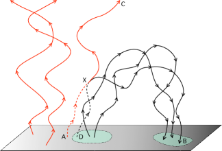
Here we suggest that similar dynamics take place everywhere at the boundary between open and closed regions where turbulent IR can occur stochastically (Figures 1-2), naturally accounting for the observed flows along and around these boundaries, including those at adjacent active region edges observed by Sakao et al. (2007), that cannot be explained by IR at the streamer apex.

In this paper we investigate the dynamics of IR at the interface between open and closed corona, with photospheric convective motions shuffling the magnetic field lines’ footpoints. For a simple first demonstration, we apply photospheric motions only to the (originally) closed region, so that no waves or turbulent dynamics are excited directly by photospheric motions along the originally open field lines.

2. Model and Governing Equations

Figure 2.— Snapshot of the simulated interface between closed (straightened out loop) and open regions of the solar Corona. Field lines are line-tied at the photospheric plane $z=0$, where convection-mimicking motions (shown in contours) are applied at $x<1$ and vanish for $x>1$. Closed field lines return to the plate $z=10$ for $x<1$ where they are line-tied to a motionless photosphere, while for $x>1$ an open boundary is realized. The plane $x=1$ is the original boundary magnetic surface between open and closed regions at $t=0$.

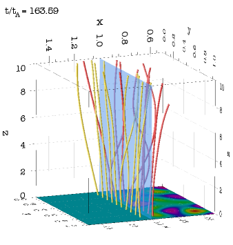
We model the interface region in Cartesian geometry (Figure 2), with a straightened loop juxtaposed with an open-field region. Curvature effects are neglected. The computational box spans $0<x<2$, $0<y<1$, and $0<z<10$ (lengths are normalized by $\ell^{\ast}=60\,\textrm{Mm}$, e.g., $z$ spans $600\,\textrm{Mm}$). The plane $z=0$ represents the photosphere where both open and closed field lines are line-tied. On the $z=0$ plane, in the $x<1$ region, convective super-granular motions are modeled by imposing a large-scale velocity pattern with all modes with wave-numbers between 3 and 4 excited with random amplitudes and normalized to have an r.m.s. value $\sim 0.5\ \textrm{km}\,\textrm{s}^{-1}$, that in physical space correspond to distorted vortical streamlines with length $\ell_{c}\sim 15\,\textrm{Mm}$. This model of footpoint motion is similar to that of Rappazzo et al. (2008), and is illustrated in the contours at the bottom of Figure 2. On the remaining region of the $z=0$ plane, where $x>1$, the velocity vanishes. The upper plane at $z=10$, in the region $x<1$, represents the photospheric plate where closed loop field lines return to, and are line-tied to a motionless photosphere. On the section of the $z=10$ plane having $x>1$, an open boundary is realized, imposing non-reflecting boundary conditions (Thompson, 1987, 1990; Vanajakshi et al., 1989), i.e., wave-like signals are allowed to propagate out toward $z>10$ with no reflection toward $z<10$ (e.g., Rappazzo et al., 2005). Along $x$ and $y$ periodic boundary conditions are used.

The above system is threaded by a strong and uniform unipolar magnetic field $\mathbf{B_{0}}=B_{0}\,\mathbf{\hat{e}}_{z}$ along $z$. The field lines traced from the bottom photospheric plane $z=0$ are considered to be either closed when they map to the top $z=10$ plate with $x<1$, or open for $x>1$. Because of a large assumed conductivity and line-tying, a field line must undergo magnetic reconnection to change connectivity. Field lines traced from the plate $z=10$ with $x<1$ map the actual closed region in the $z=0$ plane. Likewise those traced from $z=10$ with $x>1$ map the open region back to the $z=0$ plane.

As in previous work the dynamics are integrated with the (nondimensional) equations of reduced magnetohydrodynamics (MHD) (Kadomtsev & Pogutse, 1974; Strauss, 1976; Montgomery, 1982), well suited for a plasma embedded in a strong axial magnetic field:

$$\partial_{t}\mathbf{u}+\mathbf{u}\cdot\nabla\mathbf{u}=-\nabla P+\mathbf{b}\cdot\nabla\mathbf{b}+c_{{}_{\!A}}\partial_{z}\mathbf{b}+\frac{(-1)^{n+1}}{Re_{n}}\nabla^{2n}\mathbf{u},$$ (1)

$$\partial_{t}\mathbf{b}+\mathbf{u}\cdot\nabla\mathbf{b}=\mathbf{b}\cdot\nabla\mathbf{u}+c_{{}_{\!A}}\partial_{z}\mathbf{u}+\frac{(-1)^{n+1}}{Re_{n}}\nabla^{2n}\mathbf{b},$$ (2)

with $\nabla\cdot\mathbf{u}=\nabla\cdot\mathbf{b}=0$. Here, gradient and Laplacian operators have only transverse ($x$-$y$) components as do velocity and magnetic field vectors ($u_{z}=b_{z}=0$), while $P$ is the total (plasma plus magnetic) pressure, $c_{{}_{\!A}}$ is the Alfvén velocity of the axial field ($B_{0}/\sqrt{4\pi\rho_{0}}$), the plasma is assumed to have uniform density $\rho_{0}$. In the simulation presented here $c_{{}_{\!A}}=200$ (velocities are normalized by $u^{\ast}=0.5\ \textrm{km}\,\textrm{s}^{-1}$), and the numerical grid has $512\times 256\times 120$ points to achieve the long duration of $\sim 1,800$ Alfvén crossing times $\tau_{A}=L_{z}/c_{{}_{\!A}}$ ($L_{z}=10$ is the loop length), corresponding to $\sim 180$ nonlinear times, necessary to acquire significant statistics. We use hyperdiffusion with $n=4$ and $R_{4}=5\,\times 10^{16}$ that eliminates diffusion at the large scales, a critical feature in this kind of simulations that otherwise reach a diffusive regime (see, also for a more detailed description of the numerical code, Rappazzo et al., 2008).

3. Results

Initially photospheric motions induce magnetic fluctuations in the closed regions that grow linearly in time. A nonlinear, turbulent stage is attained around time $\tau_{{}_{\!NL}}\sim 10\,\tau_{A}$ (for details see Rappazzo et al., 2008). The dynamics subsequently leads to many field-aligned current sheets where magnetic reconnection occurs. These structures are highly dynamic, crossing a transverse correlation length (here, the super-granulation scale $\ell_{c}$) in approximately a nonlinear time-scale $\tau_{{}_{\!NL}}$. In this dynamic sea of current sheets, roughly half of those forming within a correlation length from the open-closed boundary will encounter it, thus changing its location and inducing changes in field-line connectivity.

Figure 3.— Field lines’ footpoints in the plane $z=10$. Field lines are traced from points with $x=x_{0}$ in the plane $z=0$. Their footpoints’ orthogonal displacement relative to their origination point (central circle) is shown for four selected values of $x_{0}$. The boundary between open and closed regions is at $x=1$.

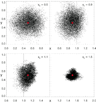
Figure 2 shows field lines at $t\sim 163.59\,\tau_{A}$ originating at $z=0$ near the initial open-closed boundary at $t=0$ ($x=1$), but which cross the boundary prior to arrival at $z=10$. This opening and closing of field lines is caused by the highly dynamic current sheets and reconnection described above. This is bursty and stochastic, and increasingly so with higher Reynolds numbers (Servidio et al., 2009).

To quantitatively understand the impact of this kind of IR we analyze the statistical properties of field lines. We ask what is the fraction of time spent in open/closed regions, or the probability for a field line traced from a point $x=x_{0}$ from the boundary in the photospheric plane $z=0$ to be closed or open when it arrives at the top plane $z=10$. The latter condition corresponds to $x<1$ or $x>1$ respectively.

To address this, we trace field lines from points in the plane $z=0$ with $x=x_{0}$ fixed. They are traced at $320$ different times, separated by $\Delta t=5\,\tau_{A}$, corresponding to approximately half a nonlinear time. To increase statistics the field lines are computed in 40 equally spaced points along $y$ (along this direction points are statistically equivalent). Figure 3 shows the footpoints’ displacement in the $x$-$y$ plane for 12,800 field lines in the plane $z=10$. Four cases correspond to four selected initial distances $x_{0}$ from the boundary. The field line tracing code (Dalena et al., 2012) employs a fifth order Runge-Kutta with adaptive step-size, and second order interpolation.

Field lines traced from the middle of the originally closed and open regions, i.e., $x_{0}=0.5$ and $1.5$, exhibit an isotropic distribution of footpoints of different extension because in the closed region magnetic fluctuations are stronger. No waves are injected from the region $z=0$ with $x>1$, but magnetic field fluctuations “leak” from the closed region, where magnetic forces push the magnetic islands against each other and these forces are unbalanced by weaker fields in the open region, with the energy density reducing across the original boundary at $x=1$. This drop in turbulence intensity along $x$ is the cause of anisotropy for the footpoints distributions for $x_{0}=0.9$ and $1.1$ that are narrower along $x$.

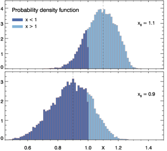
Field lines traced from $x_{0}=0.5$ and $1.5$, more distant from the initial open-closed boundary, never change connectivity from open to closed (or vice-versa). But those traced from $x_{0}=0.9$ and $1.1$ do, and their p.d.f.s are shown in Figure 4. They have a probability of $\sim 20\%$ to change connectivity from their initial type at time $t=0$. From the dynamical point of view the probability can be seen as the fraction of time the field line is closed or open.

Figure 4.— Probability density functions of the footpoints shown in Figure 3 for $x_{0}=0.9$ and $x_{0}=1.1$, across the boundary between open and closed regions at $x=1$.

Given the complex character of the magnetic field $\mathbf{b}$, which becomes broad band in space, while also evolving in time, it is natural to try to describe the spreading (and changes of connectivity) as a diffusive process. In fact there are two related diffusive processes at work. First, in Figure 2 we see that at a fixed instant of time, field lines wander randomly due to fluctuations. Second, for the spreading found in the above numerical experiment shown in Figures 3 and 4, the time dependence of the turbulence contributes an additional randomizing effect. The diffusive nature of the field line spreading is verified by the computation (not shown) of the mean square displacement $\langle\Delta x^{2}\rangle$, which increases linearly with height in the manner of diffusion:

$$\langle\Delta x^{2}\rangle=2Dz.$$ (3)

We found this linear scaling for all values of $x_{0}$, with diffusion coefficients, e.g., $D=93.6$, $56.82$ and $14.46\,\textrm{km}$ for $x_{0}=0.5$, 1, and $1.5$ respectively (normalized to $\ell^{\ast}=60\,\textrm{Mm}$).

This type of randomization of magnetic field lines is not often associated with coronal fields (usually modeled as smooth and laminar), where field lines may be line-tied at both ends. This diffusive rearrangement of connectivity requires magnetic reconnection to occur. A quantitative theory for this space-time diffusion of field lines appears to be tractable but lengthy, and we will address it in a subsequent paper (Ruffolo et al., in preparation).

Two features of the diffusion theory are pertinent at present. First, the expected $\langle\Delta x^{2}\rangle$ at height $z$ due to single time randomization – the FLRW effect – and the expected additional mean square displacement at height $z$ due to the time dependent changing of field lines, are of the same order. Second, there are two broad classes of FLRW diffusion coefficients, say $D_{ql}\sim\lambda_{z}(b/B_{0})^{2}$, the quasi-linear result (Jokipii & Parker, 1968), and $D_{Bohm}\sim\lambda_{\perp}b/B_{0}$ (Ghilea et al., 2011). Here $\lambda_{z}\sim 5$ and $\lambda_{\perp}\sim 1/4$ are suitable coherence scales in directions parallel and perpendicular to ${\bf B}_{0}$, with $b/B_{0}\sim 2\%$ in the closed region. Note that the present case of reduced MHD requires the ordering $b\lambda_{z}/(B_{0}\lambda_{\perp})\sim\tau_{\parallel}/\tau_{\perp}\sim 1$, from which $D_{Bohm}\sim D_{ql}$. Consequently we anticipate that the observed diffusive spreading (Figures 2-4) is characterized by a diffusion coefficient on the order of the quasi-linear result.

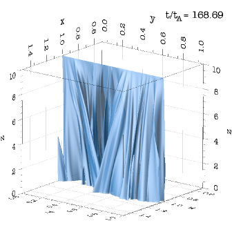
Also important is the evolving structure of the boundary between open and closed regions. At time $t=0$ the boundary is simply the plane $x=1$ (Figure 2), but at later times the magnetic surface has to be computed.

Figure 5.— Open-closed regions boundary magnetic surface.

In reduced MHD, with uniform axial field $\mathbf{B}_{0}=B_{0}\mathbf{\hat{e}}_{z}$ and transverse fluctuations $\mathbf{b}$, the magnetic surface coordinate $\psi$ obeys the magnetic differential equation

$$\partial_{z}\psi=-\frac{1}{B_{0}}\ \mathbf{b}\cdot\nabla\psi,$$ (4)

where the right side involves only the components of $\nabla$ transverse to ${\bf B}_{0}$, with initial condition $\psi(x,y,z=10)=sin(\pi x)$. The numerical code employs a third order Runge-Kutta, quadratic interpolation, and adaptive step-size.

Like a passive scalar, solutions to equation (4) can acquire a complex structure (Matthaeus et al., 1995). The boundary magnetic surface $\psi=0$ separates the two topologically different regions, and in Figure 5 it is shown at time $t=168.69\,\tau_{A}$. Its structure is fractal, appears like a pleated drape with many intricate folds, but for a continuous field $\mathbf{b}$ it does not tear no matter how folded it is, although numerically a small diffusivity removes the smallest-scale folds and minor tearing occurs. The boundary magnetic surface evolves in time and on the average its map on the plane $z=0$ has an excursion in $x$ given by twice $\langle\Delta x^{2}\rangle^{1/2}=(2DL_{z})^{1/2}$ (equation (3)), where $L_{z}$ is the loop length.

4. Conclusions and Discussion

Previous studies have shown that IR is required, e.g., to explain the quasi-rigid rotation of coronal holes in presence of the underlying photospheric differential rotation (Wang et al., 1996; Lionello et al., 2005, 2006), but this approach (see also Schrijver & De Rosa, 2003; Wang & Sheeley, 2004) assumes a quasi-steady coronal response to photospheric evolution. In the prevailing view that coronal interchange occurs at the apex of streamers and pseudo-streamers in correspondence of $Y$ or $X$-points (Wang et al., 2012), all previous simulations and modeling have used smooth large-scale fields that contain neutral points (${\bf B}=0$).

Wang et al. (1998) anticipated that field line footpoints shuffling may promote IR at the boundary between open and closed regions. The present model provides a specific mechanism for this to occur, modeling IR as component reconnection that may occur all along the magnetic interface between coronal hole and loop threaded by a unipolar field that contain no true neutral points, and extends the range of occurrence of IR proposed by Wang et al. (1998). These reconnection sites are well known in the context of nanoflare models, but their role in interchange has not been previously emphasized. Here we simulate only a small volume of the open-closed region interface to employ a higher spatial resolution. This allows the development of MHD turbulence, with its associated magnetic fluctuations in the coronal field (Figures 1 and 2), naturally induced by photospheric motions shuffling the field lines’ footpoints.

Turbulent IR renders the boundary between open and closed regions dynamic (Figures 3-5). The boundary fluctuates continuously with an average displacement of the order of the super-granulation scale $\ell_{c}\sim 15\,\textrm{Mm}$. IR can then inject loop plasma along the boundary and in the fanlike regions adjacent to closed regions, where slow streams with loop composition have been recently observed (Sakao et al., 2007; Brooks & Warren, 2011), providing an alternate mechanism to account for the plasma composition at the edges of active regions (Cranmer et al., 2007), and additional momentum, mass and energy for the streams originating from there (Wang, 1994).

In a realistic geometry the field lines originating from this small fanlike regions expand super-radially in the heliosphere and map in an extended region around the HCS. Thus flows due to turbulent IR naturally diffuse away from the HCS, overcoming the restriction of the smooth field model proposed by Antiochos et al. (2011) that admit diffusion only for streams originating from narrow open flux channels connecting two coronal holes.

In summary, when field lines’ footpoints are shuffled by photospheric motions, component magnetic reconnection is expected to occur in unipolar loop and open field regions and near the boundaries between them. This stochastic IR is likely to operate all along these boundaries and adjacent regions, where closed and open field lines can then continuously change connectivity. On this basis we suggest that plasma and energy transport along these magnetic field lines may be an important factor in generating the slow wind, and in broadening the regions in which compositional and other properties are mixed in the solar wind.

In the future we plan to extend this work to more realistic reduced and full MHD models that include curvature and expansion effects and alternate boundary conditions, allowing us to determine the relative importance of apex neutral point IR and stochastic component IR.

References

- Antiochos et al. (2007) Antiochos, S. K., Devore, C. R., Karpen, J. T., & Mikić, Z. 2007, ApJ, 671, 936
- Antiochos et al. (2011) Antiochos, S. K., Mikić, Z., Titov, V. S., Lionello, R., & Linker, J. A. 2011, ApJ, 731, 112
- Borrini et al. (1981) Borrini, G., Wilcox, J.M., Gosling, J.T., & Bame, S. J., Feldman, W.C. 1981, J. Geophys. Res., 86, 4565
- Brooks & Warren (2011) Brooks, D., & Warren, H. 2011, ApJ,727, L13
- Cranmer et al. (2007) Cranmer, S. R., van Ballegooijen, A. A., & Edgar, R. J. 2007, ApJS, 171, 520
- Crooker et al. (2002) Crooker, N. U., Gosling, J. T., Kahler, S. W. 2002, J. Geophys. Res., 107, 1028
- Dahlburg & Einaudi (2003) Dahlburg, R. B., & Einaudi, G. 2003, Adv. Space Res., 32, 1125
- Dalena et al. (2012) Dalena, S., Chuychai, P., Mace, R. L., Greco, A., Qin, G., & Matthaeus, W. H. 2012, Comput. Phys. Commun., 183, 1974
- Dmitruk & Gómez (1997) Dmitruk, P., & Gómez, D. O. 1997, ApJ, 484, L83
- Edmondson et al. (2009) Edmondson, J., Lynch, B., Antiochos, S. K., Devore, C. R., & Zurbuchen, T. 2009, ApJ, 707, 1427
- Einaudi et al. (1996) Einaudi, G., Velli, M., Politano, H., & Pouquet, A. 1996, ApJ, 457, L113
- Feldman & Widing (2003) Feldman, U., & Widing, K.G. 2003, Space Sci. Rev., 107, 665
- Fisk & Schwadron (2001) Fisk, L. A., & Schwadron, N. A. 2001, ApJ, 560, 425
- Fisk et al. (1999) Fisk, L. A., Zurbuchen, T. H., & Schwadron, N. A. 1999, ApJ, 521, 868
- Geiss et al. (1995) Geiss, J., Gloeckler, G., & von Steiger, R. 1995, Space Sci. Rev., 72, 49
- Ghilea et al. (2011) Ghilea, M., Ruffolo, D., Chuychai, P., Sonsrettee, W., Seripienlert, A., & Matthaeus, W. H. 2011, ApJ, 741, 16
- Gosling et al. (1981) Gosling, J.T., Asbridge, J.R., Bame, S.J., Feldman, W.C., Borrini, G., & Hansen, R.T. 1981, J. Geophys. Res., 86, 5438
- Howard et al. (2012) Howard, T. A., DeForest, C. E., & Reinard, A. A. 2012, ApJ, 754, 102
- Jokipii & Parker (1968) Jokipii, J. R., & Parker, E. N. 1968, Phys. Rev. Lett., 21, 44
- Jokipii & Parker (1969) Jokipii, J. R., & Parker, E. N. 1969, ApJ, 155, 777
- Kadomtsev & Pogutse (1974) Kadomtsev, B. B., & Pogutse, O. P. 1974, Sov. Phys. JETP, 38, 283
- Linker et al. (2011) Linker, J. A., Lionello, R., Mikić, Z., Titov, V. S., & Antiochos, S. K. 2011, ApJ, 731, 110
- Lionello et al. (2006) Lionello, R., Linker, J. A., Mikić, Z., & Riley, P. 2006, ApJ, 642, L69
- Lionello et al. (2005) Lionello, R., Riley, P., Linker, J. A., & Mikić, Z. 2005, ApJ, 625, 463
- Masson et al. (2012) Masson, S., Aulanier, G., Pariat, E., & Klein, K. 2012, Sol. Phys., 276, 199
- Matthaeus et al. (2007) Matthaeus, W. H., Bieber, J. W., Ruffolo, D., Chuychai, P., & Minnie, J. 2007, ApJ, 667, 956
- Matthaeus et al. (1995) Matthaeus, W. H., Gray, P. C., Pontius, D. H., & Bieber, J. W. 1995, Phys. Rev. Lett., 75, 2136
- Montgomery (1982) Montgomery, D. 1982, Phys. Scr. T, 2, 83
- Owens et al. (2008) Owens, M. J., Crooker, N. U., Schwadron, N. A., Horbury, T. S., Yashiro, S., Xie, H., St. Cyr, O. C., & Gopalswamy, N. 2008, Geophys. Res. Lett., 35, 20108
- Parker (1972) Parker, E. N. 1972, ApJ, 174, 499
- Parker (1988) Parker, E. N. 1988, ApJ, 330, 474
- Rappazzo et al. (2005) Rappazzo, A. F., Velli, M., Einaudi, G., & Dahlburg, R. B. 2005, ApJ, 633, 474
- Rappazzo et al. (2007) Rappazzo, A. F., Velli, M., Einaudi, G., & Dahlburg, R. B. 2007, ApJ, 657, L47
- Rappazzo et al. (2008) Rappazzo, A. F., Velli, M., Einaudi, G., & Dahlburg, R. B. 2008, ApJ, 677, 1348
- Sakao et al. (2007) Sakao, T. et al. 2007, Science, 318, 1585
- Schrijver & De Rosa (2003) Schrijver, C. J., & De Rosa, M. L. 2003, Sol. Phys., 212, 165
- Servidio et al. (2009) Servidio, S., Matthaeus, W. H., Shay, M. A., Cassak, P. A., Dmitruk, P. 2009, Phys. Rev. Lett., 102, 115003
- Strauss (1976) Strauss, H. R. 1976, Phys. Fluids, 19, 134
- Thompson (1987) Thompson, K. W. 1987, J. Comput. Phys., 68, 1
- Thompson (1990) Thompson, K. W. 1990, J. Comput. Phys., 89, 439
- Titov et al. (2011) Titov, V. S., Mikić, Z., Linker, J. A., Lionello, R., & Antiochos, S. 2011, ApJ, 731, 111
- Vanajakshi et al. (1989) Vanajakshi, T. X., Thompson, K. W., & Black, D. C. 1989, J. Comput. Phys., 84, 343
- Wang (1994) Wang, Y.-M. 1994, ApJ, 437, L67
- Wang et al. (2012) Wang, Y.-M., Grappin, R., Robbrecht, E., & Sheeley, N. R. 2012, ApJ, 749, 182
- Wang et al. (1996) Wang, Y.-M., Hawley, S. H., & Sheeley, N. R. 1996, Science, 271, 464
- Wang & Sheeley (2004) Wang, Y.-M., & Sheeley, N. R. 2004, ApJ, 612, 1196
- Wang et al. (1998) Wang, Y.-M., Sheeley, N. R., Walters, J. H., Brueckner, G. E., Howard, R. A., Michels, D. J., Lamy, P. L., Schwenn, R., & Simnett G. M. 1998, ApJ, 498, L165
- Winterhalter et al. (1994) Winterhalter, D., Smith, E. J., Burton, M. E., Murphy, N., & McComas, D.J. 1994, J. Geophys. Res., 99, 6667
- Zirker (1977) Zirker, J. B. 1977, Rev. Geophys. Space Phys., 15, 257
- Zurbuchen et al. (2002) Zurbuchen, T., Fisk, L. A., Gloeckler, G., & von Steiger, R. 2002, Geophys. Res. Lett., 29, 66