Point particles in 2+1 dimensions: toward a semiclassical loop gravity formulation

Abstract

We study point particles in 2+1 dimensional first order gravity using a triangulation to fix the connection and frame-field. The Hamiltonian is reduced to a boundary term which yields the total mass. The triangulation is dynamical with non-trivial transitions occurring when a particle meets an edge. This framework facilitates a description in terms of the loop gravity phase space.

1 Introduction

Three dimensional gravity has often been used as a toy model for the four dimensional theory. Here we study point particles in 2+1 dimensions using spatial geometries analogous to those in [1]. These geometries are isomorphic to a gauge-reduced holonomy-flux phase space which descends from the $\hbar\rightarrow 0$ limit of a loop quantum gravity Hilbert space.

We consider a Hamiltonian written in terms of frame-field and connection variables. The spacetime signature is taken to be Euclidean since the relevant gauge group is then $\text{SU}(2)$, as in 3+1 dimensions with Lorentzian signature. Our first step is to specify the variables over an entire spacelike slice using a triangulation where particles sit on the vertices. After gauge fixing, the Hamiltonian is reduced to a boundary term which equals the total particle mass. In this gauge the triangulation evolves according to particle momenta and undergoes discrete changes when a particle meets an edge, collapsing one of the triangles.

2 Hamiltonian formulation

Spacetime is taken to be $M=\mathbb{R}\times\Sigma$ where $\Sigma$ is a spacelike surface homeomorphic to a disc. The first order formalism of general relativity parameterizes the gravitational field in terms of a connection $\mathbf{A}$ and a frame-field $\mathbf{e}$, both being one-forms on $\Sigma$ taking values in the $\mathfrak{su}(2)$ algebra. We use $\mathfrak{su}(2)$ basis elements $\tau^{i}$ (for $i=0,1,2$) which are given by $-i/2$ times the Pauli matrices. Our notation is such that elements of $\mathfrak{su}(2)$ are written as $\mathbf{A}\equiv A^{i}\tau^{i}$, for example, and all internal indices are written as superscripts.

In units where $8\pi G=c=1$ a Hamiltonian for pure gravity is given by [2]:

$$H = -\int_{\Sigma}\left(N^{i}F^{i}+\lambda^{i}G^{i}\right)+\int_{\partial\Sigma}N^{i}A^{i},$$

$$F^{i} = \mathrm{d}A^{i}+\frac{1}{2}\epsilon^{ijk}A^{j}\wedge A^{k},$$ (1)

$$G^{i} = \mathrm{d}e^{i}+\epsilon^{ijk}A^{j}\wedge e^{k}.$$

$N^{i}$ and $\lambda^{i}$ are Lagrange multipliers for the flatness and Gauss constraints respectively. We normalize the time coordinate by choosing $|N|^{2}=1$. The boundary term and the condition $\left.\lambda^{i}\right|_{\partial\Sigma}=0$ ensure that the variational principal is well-defined and the constraints are first class. The Poisson algebra is:

$$\left\{A_{a}^{i}(x),e_{b}^{j}(y)\right\} = \epsilon_{ab}\delta^{ij}\delta^{2}(x-y),$$ (2)

where $a=1,2$ labels the space coordinates.

It is well-known that in 2+1 dimensions point particles represent conical singularities [3]. We introduce particles by replacing the flatness constraint with $F^{i}-\sum_{I}\delta^{2}(x-q_{\pi})p_{\pi}^{i}\mathrm{d}x^{2}$ so that each particle $\pi$ gives a contribution to the curvature proportional to its momentum $\mathbf{p}_{\pi}$ at the location $x=q_{\pi}$ [2]. In this treatment the particles are defined by the fields $(\mathbf{A},\mathbf{e})$ and do not have independent parameters of their own. We consider the total mass to be less than $2\pi$ so that $\Sigma$ is open [3].

3 Gauge fixing

In order to solve the constraints and reduce the Hamiltonian, we triangulate $\Sigma$ according to the particle locations so that we may give a piecewise definition of $(\mathbf{A},\mathbf{e})$ on $\Sigma\setminus\left\{q_{\pi}\right\}$. See [4] for other approaches along these lines. For clarity, we take the boundary $\partial\Sigma$ to be triangular; the generalization to arbitrary polygons follows simply. We take each particle position to be an internal vertex and connect all vertices with straight edges to obtain a triangulation. There is ambiguity in this procedure, but the number of triangles $T$ is fixed by the number of particles $\Pi$ to be $T=2(\Pi+1)-1$ via the Euler characteristic for planar graphs. Different triangulations generally lead to different gauge choices.

Within each triangle $\Delta$, we must choose $(\mathbf{A}_{\Delta},\mathbf{e}_{\Delta})$ such that $G^{i}=F^{i}=0$. The general solution [1] is given by an $\text{SU}(2)$ group element $a_{\Delta}$ and a closed one-form ${\bm{\chi}}_{\Delta}$:

$$\mathbf{A}_{\Delta}=a_{\Delta}\mathrm{d}a_{\Delta}^{-1},\hskip 36.135pt\mathbf{e}_{\Delta}=a_{\Delta}{\bm{\chi}}_{\Delta}a_{\Delta}^{-1}.$$ (3)

Consider two adjacent triangles labeled $1$ and $2$. We ensure that the fields are continuous across the shared edge $e$ by requiring that there exists an $h_{e}\in\text{SU}(2)$ on the edge such that:

$$\left.a_{2}\right|_{e}=\left.a_{1}h_{e}\right|_{e},\hskip 36.135pt\left.{\bm{\chi}}_{2}\right|_{e}=\left.h_{e}^{-1}{\bm{\chi}}_{1}h_{e}\right|_{e}.$$ (4)

Now, if we integrate the curvature over a region containing a single vertex $\pi$ we must obtain $\int F^{i}=p_{\pi}^{i}$. In order to specify the group elements $a_{\Delta}$ we subdivide each triangle into three regions defined by edges joining the centroid to the vertices. Consider one such region $\Delta_{r}$ where points $(0,\pm y_{0})$ are the endpoints of an edge, and $(x_{0},y_{1})$ is the centroid of the triangle. We define:

$$u=\tanh^{-1}(v_{+})+\tanh^{-1}(v_{-}),$$ (5)

where $v_{\pm}=\frac{x}{x_{0}}\pm\left(\frac{y}{y_{0}}-\frac{xy_{1}}{x_{0}y_{0}}\right)$. Note that the line $u=0$ coincides with the edge, and $u=\infty$ consists of lines between the centroid of the triangle and the endpoints of the edge. We set the group element in a region equal to:

$$a_{\Delta_{r}}(u)=\exp\left(\mathbf{P}\int_{0}^{u}f(\tilde{u})\mathrm{d}\tilde{u}\right),$$ (6)

where we have introduced a bump function $f(u)$ which satisfies $\int_{0}^{\infty}f(u)\mathrm{d}u=1$. For a given $u$, this group element defines a rotation about a direction $\mathbf{P}/|P|$ by an angle proportional to $|P|$.

With these ingredients it is now possible to choose a gauge, i.e. to specify the frame-field and connection on $\Sigma\setminus\left\{q_{\pi}\right\}$. Given a set of particles $\left\{q_{\pi},p_{\pi}\right\}$, one first defines a boundary and introduces a triangulation. Then we arbitrarily choose a triangle (labeled 1) and make a choice for $(a_{1},{\bm{\chi}}_{1})$. Moving to a neighbouring triangle, we specify $a_{2}$ here and use (4) to find ${\bm{\chi}}_{2}$. We continue in this manner until $(a_{\Delta},{\bm{\chi}}_{\Delta})$ (and thereby $(\mathbf{A}_{\Delta},\mathbf{e}_{\Delta}))$ are defined in each triangle, taking care to ensure the connection yields proper curvature at each vertex by choosing the parameter $\mathbf{P}$ in each $a_{\Delta_{r}}$ to be consistent with particle momenta. The aforementioned relationship between the number of triangles and the number of particles ensures that this procedure will work for arbitrarily many particles. See [5] for a more detailed description of this process.

Preserving the gauge dynamically leads to a condition on the Lagrange multipliers:

$$\mathrm{d}_{A}N^{i}+\epsilon^{ijk}e^{j}\lambda^{k}=0.$$ (7)

This fixes three of the six degrees of freedom in $N^{i}$ and $\lambda^{i}$. We eliminate the remaining ambiguity by choosing $\mathrm{d}_{A}N^{i}=0$ and setting $\mathbf{N}(q_{\pi})=\mathbf{p_{\pi}}/m$. This choice ensures that particles move along with the triangulation and remain at the vertices.

4 Dynamics and observables

After specifying $(\mathbf{A},\mathbf{e})$, the Hamiltonian is reduced to a boundary term which evaluates to:

$$H = \int_{\partial\Sigma}N^{i}A^{i}=\int_{\Sigma}N^{i}\mathrm{d}_{A}A^{i}$$ (8)

$$= \sum_{\pi}N^{i}(q_{\pi})p_{\pi}^{i}=\sum_{\pi}m_{\pi},$$

where we used Stokes’ theorem, the conditions on $\mathbf{N}$, and the flatness constraint.

Dynamics are implicitly determined by the direction of momentum $N^{i}(q_{\pi})$ for each particle via the equation of motion:

$$\dot{q}_{\pi}^{i}(t)=q_{\pi}^{i}(0)+tN^{i}(q_{\pi}),$$ (9)

and the triangulation evolves accordingly. Non-trivial, discrete transitions occur when a particle meets an edge. Consider triangles $1$ and $2$ depicted in fig. 1.

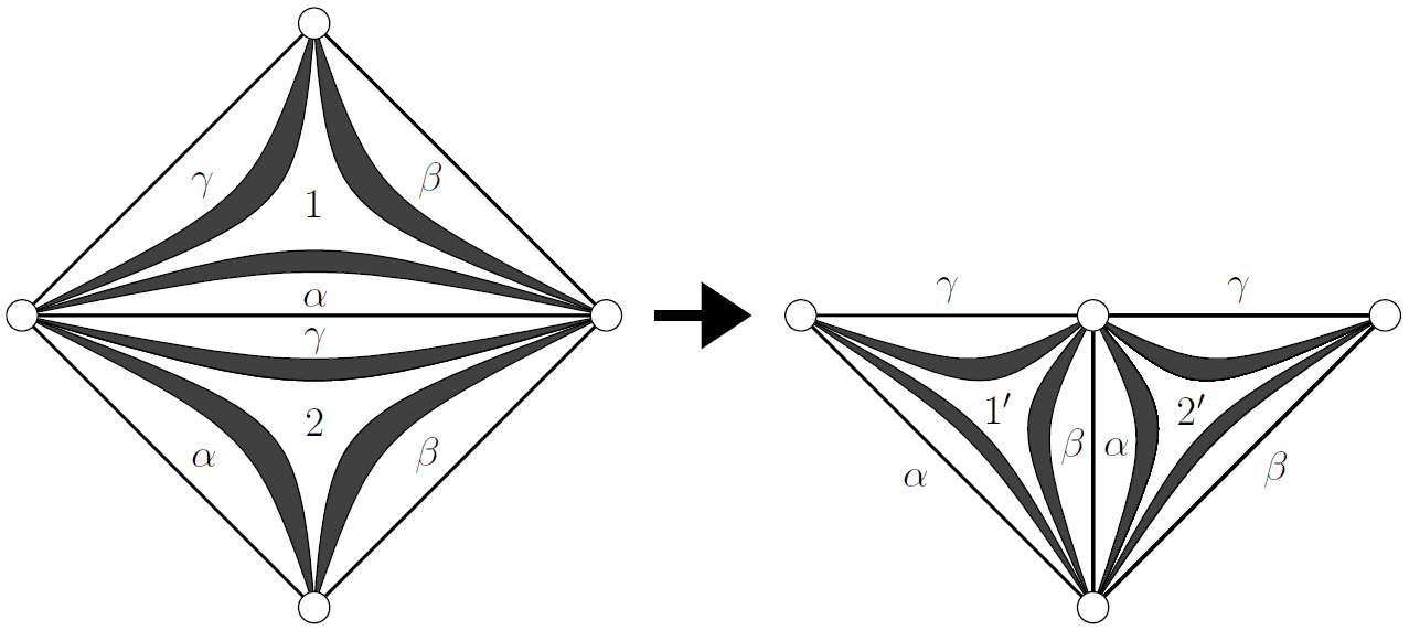
Figure 1: Before and after a discrete change in triangulation. $\alpha,\beta,\gamma$ label the three regions of each triangle. Grey regions (bounded by constant-$u$ lines) indicate where the connection is generally non-zero.

If the particle at the top of the left hand side of the figure moves downward until it reaches the shared edge, then $1$ closes and $2$ splits into $1^{\prime}$ and $2^{\prime}$ (shown on the right hand side) preserving the total number of triangles. The fields are defined in the new triangles by specifying the $\text{SU}(2)$ rotation parameters:

$$\mathbf{P}_{1^{\prime}_{\gamma}}=\mathbf{P}_{1_{\alpha}}+\mathbf{P}_{2_{\gamma}}+\mathbf{P}_{1_{\gamma}},\hskip 18.06749pt\mathbf{P}_{1^{\prime}_{\alpha}}=\mathbf{P}_{2_{\alpha}},$$

$$\mathbf{P}_{2_{\gamma}^{\prime}}=\mathbf{P}_{1_{\alpha}}+\mathbf{P}_{2_{\gamma}}+\mathbf{P}_{1_{\beta}},\hskip 18.06749pt\mathbf{P}_{2_{\beta}^{\prime}}=\mathbf{P}_{2_{\beta}},$$ (10)

$$\mathbf{P}_{1_{\beta}^{\prime}}=\mathbf{P}_{2_{\alpha}^{\prime}}=0.$$

Notice $h_{e}=\mathbb{1}$ along the new edge shared by $1^{\prime}$ and $2^{\prime}$ so that ${\bm{\chi}}_{1^{\prime}}={\bm{\chi}}_{2^{\prime}}={\bm{\chi}}_{2}$. The fields in all other triangles are unaffected by this transition.

5 Conclusion

We have described a system of point particles in 2+1 dimensional gravity in terms of evolving triangulations. A gauge choice for $(\mathbf{A},\mathbf{e})$ was specified by choosing $a_{\Delta}$ and ${\bm{\chi}}_{\Delta}$ in each triangle. The triangulation evolves according to particle dynamics so that particles remain at vertices at all times. The discrete change in triangulation that occurs when a vertex meets an edge is well-defined.

This construction yields spatial geometries that are the two-dimensional analog of those in [1]. Having $(a_{\Delta},{\bm{\chi}}_{\Delta})$ in each triangle allows us to immediately write this data in terms of holonomy-flux variables. Moreover, knowing how $(a_{\Delta},{\bm{\chi}}_{\Delta})$ behave under a discrete change in triangulation tells us how the holonomies and fluxes will change. This sets the stage for a semiclassical loop gravity description of the system [5].

Acknowledgements: The author is grateful to Gabor Kunstatter, Laurent Freidel and John Moffat for helpful conversations during the course of this work.

References

- [1] L. Freidel, M. Geiller and J. Ziprick, arXiv:1110.4833v1 [gr-qc] (2011).
- [2] L. Freidel and D. Louapre, Class. Quant. Grav. 21, 5685 (2004).
- [3] S. Deser, R. Jackiw and G. ’t Hooft, Annals of Physics 152, Issue 1, 220 (1984).
- [4] G. ’t Hooft, Class. Quantum Grav. 9 1335 (1992); H.J. Matschull, Class. Quant. Grav. 18, 3497 (2001).
- [5] J. Ziprick, in preparation.