A Study of the Orbits of the Logarithmic Potential for Galaxies

Abstract

The logarithmic potential is of great interest and relevance in the study of the dynamics of galaxies. Some small corrections to the work of Contopoulos & Seimenis (1990) who used the method of Prendergast (1982) to find periodic orbits and bifurcations within such a potential are presented. The solution of the orbital radial equation for the purely radial logarithmic potential is then considered using the p-ellipse (precessing ellipse) method pioneered by Struck (2006). This differential orbital equation is a special case of the generalized Burgers equation. The apsidal angle is also determined, both numerically as well as analytically by means of the Lambert $W$ and the Polylogarithm functions. The use of these functions in computing the gravitational lensing produced by logarithmic potentials is discussed.

1 Introduction

The logarithmic potential has great interest in connection with the dynamics of elliptical galaxies and galactic halos. Introduced by Richstone (1980) to model stellar systems with concentric axisymmetric oblate spheroidal potential surfaces, it is one of the few axisymmetric galactic potentials with an equally simple mass distribution function. As a result it has been studied extensively (e.g. Binney & Spergel (1982); Binney & Tremaine (1987)).

Richstone (1982) did an extensive survey of orbits within scale-free logarithmic potentials (that is, with zero core radii). The effect of core radius and the presence or absence of a central mass have been examined by Gerhard & Binney (1985); Pfenniger & de Zeeuw (1989); Miralda-Escude & Schwarzschild (1989). Evans (1993) examined the axisymmetric case of galaxies embedded in extended dark matter halos. Lees & Schwarzschild (1992) examined triaxial halo models. Karanis & Caranicolas (2001) examined how the core radius and the angular momentum are related to transitions from regular motion to chaos in log potentials. Touma & Tremaine (1997) developed a symplectic map to study the dynamics of orbits in non-spherical potentials, with particular emphasis on the logarithmic potential. Periodic orbits in triaxial logarithmic potentials have been examined analytically Belmonte et al. (2007); Pucacco et al. (2008) and numerically Magnenat (1982).

Beyond galactic dynamics, the potential also has applications to the problem of gravitational lensing. Beyond astrophysics, applications of the logarithmic potential occur in the solution of planar boundary value problems in potential theory Evans (1927) and with boundary value problems of analytic function theory. In elementary particle physics, Quigg & Rosner (1977) use the logarithmic potential to show that the quarkonium level spacings are independent of quark mass, in the non-relativistic limit. In this paper, the analysis of Contopoulos & Seimenis (1990) (CS) is re-examined. CS applied the analytical techniques of Prendergast (1982) to find approximate solutions to the equations of motion for particles moving within a logarithmic potential. The Prendergast method was introduced to approximate some complex differential equations, such as the Duffing equation, and new applications for this method are still being found today. We then elaborate on the work of CS, turning our attention to the radial orbital equation, using the nonlinear Burgers equation to determine an approximate analytic solution from which the apsidal angle is determined. It is also determined by finding the roots of the Lambert $W$ and the polylogarithmic function.

In sections 2 and 3, the Prendergast Method is revisited. We performed a thorough study of the pioneering work of Contopoulos & Seimenis (1990) and present a slight elaboration as well as a few minor corrections to their equations. In section 4, we briefly study Struck (2006)’s p-ellipse (precessing ellipse), introduced in his fine work on precessing orbits in a variety of power-law potentials, some shallower than the $1/r$ Keplerian one. These potentials include the logarithmic potential of zero as well as nonzero core softening length. We present an integrable equation that provides us with values for the apsidal angles of the orbits considered. In section 5 we discuss the deflection of light in a logarithmic potential and gravitational lensing. Finally, section 6 summarizes our conclusions and any further work to be considered.

2 Unperturbed Solutions

Here we begin by re-establishing the results of CS with some minor corrections, before going on to use these solutions in subsequent sections. Where alterations to their values are given, they are indicated by asterisks.

Following the notation of CS, our expression for the logarithmic potential is

$$V(x,y)=\ln\left(x^{2}+\frac{y^{2}}{U^{2}}+C^{2}\right)$$ (1)

where $C$ is the core radius and $U$ describes the ellipticity of the potential. Though of mathematical interest over a wider range of parameters, models with $U>1.08$ or $U<1/\sqrt{2}=0.707$ are unphysical in that they require negative mass densities Evans (1993). As a result, only values of $0.707<U<1.08$ are of interest to galactic dynamics. The CS method begins by finding a solution for arbitrary values of $U$ in the one-dimensional case ($y\equiv\dot{y}\equiv 0$), and adding the motion in the second dimension as a perturbation.

By finding the derivative of Eq. 1 and introducing it in the relevant second order orbital differential equation, it is possible to develop two equations of motion–one for the $x$ component, the other for the $y$ component:

$$x^{\prime\prime}+\frac{2U^{2}x}{U^{2}x^{2}+y^{2}+C^{2}U^{2}}=0$$ (2)

$$y^{\prime\prime}+\frac{2y}{U^{2}x^{2}+y^{2}+C^{2}U^{2}}=0\hskip 21.33955pt(*)$$ (3)

where the $(*)$ indicates the equation contains a correction to a typo in CS’s original.

The subsequent solution is developed using the method of Prendergast (1982). Developed for second-order nonlinear ordinary differential equations, Prendergast applied the technique to the van der Pol oscillator and Duffing’s equation. CS applied it to the orbital equation in the logarithmic potential.

The method begins by assuming a solution for $x$ and $y$ of the following form:

$$x=\frac{N}{D};\indent y=\frac{M}{D};\indent$$ (4)

where $N$, $M$ and $D$ are Fourier series of the form

$$N = \sum_{k={\rm odd}}N_{k}\cos(k\omega t),$$

$$D = 1+\sum_{l={\rm even}}D_{l}\cos(l\omega t)$$ (5)

and which are truncated at the appropriate order. In the unperturbed one-dimensional case, $y=\dot{y}=0$ and $M=0$.

In determining the solution for $x$, we introduce the expansion of 4 into Eq. 2, and solve for a new equation of motion,

$$(N^{\prime\prime}D^{2}-2N^{\prime}D^{\prime}D-ND^{\prime\prime}D+2ND^{\prime 2})\times$$

$$(U^{2}N^{2}+M^{2}+C^{2}U^{2}D^{2})+2U^{2}ND^{4}=0.$$ (6)

A solution is essayed of the form

$$N=A\cos(\omega t);\indent D=1+B\cos(2\omega t);$$ (7)

with constants $A$, $B$ and $\omega$ to be determined, though we require $B\neq 0$ for a non-trivial rational approximation.

Finally, we introduce the proposed solutions 7 into Eq. 6 and set equal to zero the coefficients of $\cos(\omega t)$ and $\cos(3\omega t)$. This gives us two equations

$$\omega^{2}k_{1}+0.75B^{4}+3B^{3}+6B^{2}+4B+2 = 0$$

$$\omega^{2}k_{2}+0.5B^{4}+3B^{3}+3B^{2}+4B = 0\hskip 21.33955pt(*)$$ (8)

where $k_{1}$ and $k_{2}$ are given below;

$$k_{1} = 3.5625A^{2}B^{2}+7B^{2}C^{2}+2.125C^{2}B^{4}-$$

$$2BC^{2}+3.5C^{2}B^{3}-0.75A^{2}-C^{2},$$

$$k_{2} = 0.1875A^{2}B^{2}+1.25A^{2}B-0.25A^{2}+$$

$$6.5C^{2}B^{3}-3.5B^{2}C^{2}+2BC^{2}+0.25C^{2}B^{4}.\hskip 7.11317pt(*)$$

The third equation needed to determine $A$, $B$ and $\omega$ is given by the initial condition

$$(1+B)x_{0}-A=0$$ (11)

where $x_{0}\equiv x(t=0)$.

We now solve these equations for $A$, $B$ and $\omega$ with the given values of $x_{0}$. The solutions, as well as all mathematical manipulations presented in this paper unless otherwise mentioned, were determined using the software package Maple 15. The solutions have $\omega^{2}$ $>$ 0 and are presented in Table 1.

	$x_{0}$	$A$	$B$	$\omega$
1	0.001	0.001000006	6.2497E-6	14.142
2	0.01	0.01000621694	0.0006216935078	14.089
3	0.02	0.02004895506	0.002447752803	13.935
4	0.03	0.03016097774	0.005365924678	13.689
5	0.04	0.04036817727	0.00920443171	13.368
6	0.05	0.05068761968	0.01375239358	12.989
7	0.06	0.06112700808	0.01878346808	12.569
8	0.07	0.07168549791	0.02407854158*	12.125
		(0.024074)
9	0.08	0.08235549842	0.02944373*	11.668
		(0.029436)
10	0.09	0.09312493232*	0.03472147*	11.211
		(0.093124)	(0.034708)
11	0.1	0.1039794453*	0.039794453*	10.761
		(0.103977)	(0.039775)
12	0.125	0.13139283*	0.05114264*	9.696
		(0.131388)	(0.051102)
13	0.15	0.1590498684*	0.060332456*	8.747
		(0.159040)	(0.060266)
14	0.175	0.1868185967*	0.067534838*	7.921
		(0.186803)	(0.067443)
15	0.2	0.2146246114*	0.073123057*	7.210*
		(0.214602)	(0.073008)	(7.209)
16	0.225	0.2424301778*	0.077467457*	6.597
		(0.242400)	(0.077332)
17	0.25	0.27021796*	0.08087184*	6.068
		(0.270180)	(0.080719)

Table 1: A comparison of our results with those of Contopolous and Seimenis (1990). Where a corrected value appears, the original value appears in brackets below it.

We note that for motion solely in the $x$-direction the value of $U$ is irrelevant, and it appears neither in Eq. 8 nor in the initial conditions.

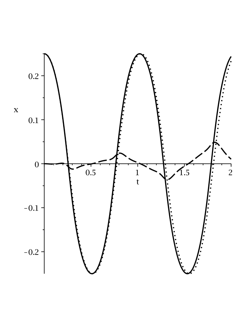
Figure 1: A typical solution showing $x$ versus time for the unperturbed solution based on the values of line 17 in Table 1. The solid line is the numerical solution from Maple 15, the dotted line is our approximation, and the dashed line is the difference between the two.

An example of an unperturbed solution is displayed in Figure 1 with values corresponding to line 17 in Table 1.

3 Perturbed Solutions

Purely radial orbits such as those of Section 2 are unlikely in practice. Here the search is for solutions to the motion where the $y$-component of the motion is close to the unperturbed motion discussed previously. In this case, $M$ is no longer identically zero and we look for solutions of the form

$$M=M_{0}+\delta M;\indent D=D_{0}+\delta D;\indent N=N_{0}+\delta N$$ (12)

where the subscript 0 indicates the unperturbed solution. The next step is to solve the differential equation, introduced as Eq. 8 in Contopoulos & Seimenis (1990)

$$(U^{2}N^{2}D^{2}+C^{2}U^{2}D^{4})\delta M^{\prime\prime}-$$

$$\ (2U^{2}N^{2}DD^{\prime}+2C^{2}U^{2}D^{3}D^{\prime})\delta M^{\prime}+$$

$$(2U^{2}N^{2}D^{\prime 2}-U^{2}N^{2}DD^{\prime\prime}-C^{2}U^{2}D^{3}D^{\prime\prime}+$$

$$2C^{2}U^{2}D^{2}D^{\prime 2}+2D^{4})\delta M=0.$$ (13)

The proposed solutions from Eq. 5 are substituted into Eq. 13 and solutions of the form

$$\delta M=\sum_{k=-\infty}^{\infty}C_{k}\cos\left(\left(\nu+k\right)\omega t\right)$$ (14)

are searched for, where $\nu$ is a constant. CS determined from Floquet (1883)’s work that values outside the range $0\leq\nu\leq 1/2$ are unstable, and thus that $\nu(x_{0})=0$ and $\nu(x_{0})=1/2$ bracket the stable region. They found no solution in the case of $\nu=0$, but solutions do exist for the case $\nu=1/2$, discussed below.

In order to get a finite number of non-trivial solutions, Eq. 14 must be truncated after a finite number of terms. Following CS we take

$$\delta M=\sum_{k=-3}^{2}C_{k}\cos\left(\left(k+\frac{1}{2}\right)\omega t\right)$$ (15)

which leaves us with six values of $C_{k}$ to be determined.

The main goal here is to solve for the six constants $C_{k}$. In order to do this, we substitute Eq. 15 and its derivatives into Eq. 13, as well as the corresponding substitutions for $N$ and $D$. From this point on, we diverge from the treatment of CS, as here we have used different methods to find this equation’s solutions. Here we used Maple 15 and Mathematica 8 as tools for equation solving.

1) Using Maple’s COMBINE function, Eq. 13 was solved for one value of $C_{k}$. The solution revealed many cosine terms with different frequencies, and some terms that were fully independent of the cosine.

2) The three lowest frequencies of cosine (including the independent terms when present) were factored out of each individual $C_{k}$ term. The terms relating to a single frequency were collected, yielding three separate equations. The cosine was then factored out, and the remainder of the equations set equal to zero.

3) Steps 1 and 2 were repeated for each individual term of $C_{k}$. The result was 18 equations where there were 3 equations for each $C_{k}$ (each of the three equations representing a different frequency of cosine). Using these equations, a $6\times 6$ matrix results, where rows 1, 3 and 5 represent equations with $k$ values of -3, -1, 1 and rows 2, 4, 6 represent equations with $k$ values of -2, 0, 2.

$$\left[\begin{array}[]{cccccc}{\it S_{11}}&0&{\it S_{13}}&0&{\it S_{15}}&0\\ \vskip 6.0pt plus 2.0pt minus 2.0pt\cr 0&{\it S_{22}}&0&{\it S_{24}}&0&{\it S_{26}}\\ \vskip 6.0pt plus 2.0pt minus 2.0pt\cr{\it S_{31}}&0&{\it S_{33}}&0&{\it S_{35}}&0\\ \vskip 6.0pt plus 2.0pt minus 2.0pt\cr 0&{\it S_{42}}&0&{\it S_{44}}&0&{\it S_{46}}\\ \vskip 6.0pt plus 2.0pt minus 2.0pt\cr{\it S_{51}}&0&{\it S_{53}}&0&{\it S_{55}}&0\\ \vskip 6.0pt plus 2.0pt minus 2.0pt\cr 0&{\it S_{62}}&0&{\it S_{64}}&0&{\it S_{66}}\end{array}\right]$$ (16)

In other words, the columns are in increasing order from -3 to 2, which demonstrates which equations contain which $k$ values.

We now solved the equations in sets of three for the values of $C_{k}$. In essence, we constructed equations from the matrix (e.g. $S_{11}+S_{13}+S_{15}=0$ and so forth down the rows). Rows 1, 3, 5 were used to solve for $C_{-3}$, $C_{-1}$ and $C_{1}$. Similarly, rows 2, 4, 6 were used to solved for $C_{-2}$, $C_{0}$ and $C_{2}$. The two homogeneous sets of three equations were transformed to two non-homogeneous systems of order two with $C_{-1}$ and $C_{0}$ set equal to unity for mathematical convenience.

Once all six coefficients were determined, the values for $x(t)$ and $y(t)$ could be determined for specific sets of values of $A$, $B$ and $\omega$ from Table 1. We then use the relations that $u=\frac{1}{r}$, and that $r=\sqrt{x^{2}+y^{2}}$ to solve for $u$.

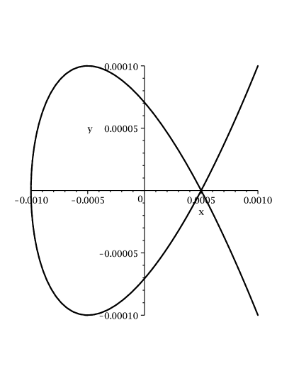
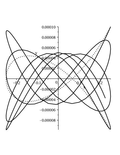
Figure 2: Two solutions showing $x$ and $y$ as a parametric curve in $t$. The left panel shows the Prendergast and real solutions based on the values of line 1 in Table 1. The two solutions plot on top of each other at this resolution and cannot be distinguished. The right panel shows a larger orbit, corresponding to the values of line 17 in Table 1. The solid curve is the numerical solution from Maple 15 over a four cycles and the dotted line is the Prendergast approximation.

Figure 2 shows two examples of a perturbed solution. In the left panel, a parametric plot in $t$ of $x$ versus $y$ for parameters $U=2/3$, $C$=0.1, and other values corresponding to line 1 in Table 1 is shown. Here the initial value of $y$ is taken to be $10^{-4}$ to justify our assumption that it is small. The two solutions are so similar that the graphs overplot each other and cannot be distinguished. The right panel shows a much larger orbit based on the parameters in line 17 of Table 1. Here the Prendergast solution does not contain enough frequency information to completely reproduce the box orbit but captures some of the character of the true solution, such as the $x$ and $y$ amplitudes and period.

4 The Apsidal Angle and p-Ellipse Orbits

In this section, we turn our interest to the approximate solution of the radial orbital differential equation. We are interested primarily in precession of the apsidal angle, and so we will consider the problem now in terms of the anomaly $\theta$ rather than the time $t$. If one wished to determine the relationship between these two variables, a Kepler-like equation would need to be solved.

CS considered the $x$ and $y$ equations of motion, but here we consider $u=1/\sqrt{x^{2}+y^{2}}=1/r$ with an eye to later using this result to determine the apsidal angle for the purely radial logarithmic potential. In this case, we examine the case where $U\approx 1$ and $C\ll 1$. We start with the radial orbital differential equation, which is of the form,

$$\frac{d^{2}u}{d\theta^{2}}+u=-\frac{1}{h^{2}u^{2}}f\left(\frac{1}{u}\right)$$ (17)

where $h$ is the angular momentum. We note that the force function $f(\frac{1}{u})$ is equal to $-dV/dr$, which can be obtained by differentiating Eq. 1.

The Prendergast Method works very well for the solutions of the logarithmic potentials from Eq. 1 indicated in Section 2 for the $x$ and $y$ equations of motion and further elaborated in Section 3. However, the method does not seem to be well suited for purely radial logarithmic potentials with different initial conditions, and the solution does not agree with that obtained by pure numerical integration of the orbital differential equation. The p-ellipse approximate solutions of the orbital equation, pioneered by Struck (2006), is a much better way of not only deriving an accurate approximate solution to order $e^{2}$ (where $e$ is the orbital eccentricity), but also obtaining the values for the apsidal precession to a high accuracy. We present a detailed analysis of the orbital equation for the radial logarithmic potential with or without the inclusion of the core scale length. In our analysis, the factor $0\leq C\leq 1$ gives a measure of the core scale length Struck (2006).

For the case of large orbits, or negligible core size softening length, the equation of motion is given by

$$uu^{\prime\prime}+u^{2}=c$$ (18)

where the parameter $c$, in the notation of Struck, depends both on the constant scale mass $M^{*}$ and the core scale length $\varepsilon$ of the potential, the gravitational constant $G$, and the angular momentum $h$. The above equation is similar to Eq. 17, and of the form

$$u^{\prime\prime}+u=\frac{c}{u}$$ (19)

Struck suggested an approximate solution of Eq. 19

$$u=\frac{1}{p}\left\{1+e\cos\left[\left(1-b\right)\phi\right]\right\}^{1/2}$$ (20)

Here, $p=a(1-e^{2})$ is the semilatus rectum; $a$ is the semi major axis ($e.~{}g.$ Murray & Dermott (1999); Valluri et al. (2005)), $e$ is the orbital eccentricity, and $(1-b)$ is the factor associated with the precession rate. Henceforth, for convenience, we set $k=1-b$ in our analysis, and we will use $\theta$ instead of $\phi$ as was used by Struck.

Struck finds that orbits obtained from a numerical integration of the above differential equation look like precessing ellipses (p-ellipses) and considers the approximate solution given in Eq. 20.

Substituting the solution of Eq. 20 into the differential equation, we find that

$$-\frac{k^{2}}{2p^{2}}\left[-\frac{e^{2}-1}{2\left(1+e\cos k\theta\right)}+\frac{1+e\cos k\theta}{2}\right]+\frac{1+e\cos k\theta}{2p^{2}}=c$$ (21)

$$\therefore uu^{\prime\prime}+u^{2}=\frac{k^{2}}{2p^{2}}\frac{1-e^{2}+\frac{1}{p^{2}}(1-\frac{k^{2}}{4})(1+e\cos k\theta)}{2(1+e\cos k\theta)}=c$$ (22)

The LHS of Eq. 22 simplifies to

$$uu^{\prime\prime}+u^{2} = -\frac{1}{2p^{2}}\left(1+e\cos k\theta\right)+\frac{1}{p^{2}}\left(1+e\cos k\theta\right)+$$ (23)

$$\frac{1}{2p^{2}}\left(1-e^{2}\right)\frac{1}{1+e\cos k\theta}=c$$

Where $c_{1}=\frac{1}{2p^{2}}+\frac{1}{2p^{2}}=\frac{1}{p^{2}}$ and $k^{2}=(1-b_{1})^{2}=2$ are the first approximations to $k$ and $c$ Struck (2006). In a more accurate approximation to order $e^{2}$, we find that the constant terms reduce to

$$\frac{k^{2}}{4p^{2}}\left(1-e^{2}\right)-\frac{k^{2}}{4p^{2}}+\frac{1}{p^{2}}=c$$ (24)

Comparing next, the terms involving $\cos k\theta$, we find that the coefficient of $\cos k\theta$ is given by

$$-\frac{k^{2}}{4p^{2}}e\left(1-e^{2}\right)-\frac{k^{2}e}{4p^{2}}+\frac{e}{p^{2}}=0$$ (25)

On simplification, one obtains

$$k^{2}=\frac{2}{1-\frac{1}{2}e}=2\left(1+\frac{e}{2}+\frac{e^{2}}{4}\right)$$ (26)

For $e=0$, $k^{2}=2$ in accord with Struck (2006).

In the case of non negligible core size, one has a similar though modified differential equation of the form

$$(uu^{\prime\prime}+u^{2})(1+u^{2})=c$$ (27)

The solution given in Eq. 20 upon substitution into the above differential equation leads to the expression

$$\left[-\frac{k^{2}}{4p^{2}}\left(1+e\cos k\theta\right)+1+\frac{e\cos k\theta}{p^{2}}+\frac{k^{2}}{4p^{2}}\frac{\left(1-e^{2}\right)}{1+e\cos k\theta}\right]\times$$

$$\left(1+\frac{1+e\cos k\theta}{p^{2}}\right)=c$$ (28)

which, upon comparison of terms independent of $\cos k\theta$, simplifies to

$$\frac{1}{p^{2}}\left(1-\frac{k^{2}e^{2}}{4}\right)\left(1+\frac{1}{p^{2}}\right)+\frac{k^{2}}{4p^{2}}\left(1-e^{2}\right)\left(1+\frac{1}{p^{2}}\right)\left(-\frac{e^{2}}{2}\right)+$$

$$\frac{k^{2}}{4p^{2}}\left(1-e^{2}\right)\left(-\frac{e^{2}}{2p^{2}}\right)=c$$ (29)

Comparing coefficients of $\cos k\theta$, we get the more general dependence of $k^{2}$.

$$k^{2}=2\left[1+\frac{\frac{e^{2}}{2}+\frac{1}{p^{2}}}{1+\frac{1}{p^{2}}-\frac{e^{2}}{2}}\right]$$ (30)

If terms of order $e^{2}$ are ignored,

$$k^{2}=1-b_{1}=2\left(\frac{1+\frac{2}{p^{2}}}{1+\frac{1}{p^{2}}}\right)$$ (31)

where $b_{1}$ is the first approximation of the precession factor.

Furthermore, to order $e^{4}$

$$c = \frac{1}{p^{2}}\left(1+\frac{1}{p^{2}}\right)-\frac{k^{2}e^{2}}{4p^{2}}\left(\frac{3}{2}+\frac{1}{p^{2}}+\frac{2}{p^{2}}\right)+$$ (32)

$$\frac{k^{2}e^{4}}{8p^{2}}\left(1+\frac{2}{p^{2}}\right)$$

in agreement with Struck.

It is interesting to note that the orbital differential equation associated with apsidal precession is a special case of the generalized Burgers partial differential equations (GBE) and seems to characterize these equations similar to the way that Painleve equations represent the Korteweg-de Vries type of equations Sachdev (1991). This variety of equations can be expressed as Eqs. 33 and 34 where $f(x)$ and $g(x)$ are sufficiently smooth arbitrary functions, $a,e$ and $c$ are real constants, and the solutions of $y$ are Euler-Painleve transcendents Kamke (1943).

$$yy^{\prime\prime}+ay^{\prime 2}+f(x)yy^{\prime}+g(x)y^{2}+ey^{\prime}+c=0$$ (33)

In the case where $f(x)$ and $g(x)$ are constants, we have the Euler-Painleve equation

$$yy^{\prime\prime}+ay^{\prime 2}+byy^{\prime}+cy^{2}+dy^{1-\alpha}=0$$ (34)

For $\alpha=1,b=0$, the substitution $y=u^{1/2}$ leads to the differential equation

$$-\frac{1}{4}\frac{u^{\prime 2}}{u}+\frac{1}{2}u^{\prime\prime}+cu+d+\frac{a}{4}\frac{u^{\prime 2}}{u}=0$$ (35)

For $a=1$ the $\frac{u^{\prime 2}}{4u}$ terms cancel, and the following equation results.

$$\frac{1}{2}u^{\prime\prime}+cu+d=0$$ (36)

It is important to observe that the orbital differential equation does not have the $ay^{\prime 2}$ term in contrast to the GBE. This term contains terms of order $e^{2}$ and the correction does not turn out to be significant. Hence, the $p$ ellipse is a natural approximate solution of the generalized Burgers equations (GBE) and is an Euler – Painleve transcendant Kamke (1943).

As a rough estimate of the mean error in neglecting the $\frac{u^{\prime 2}}{4u}$ term, we evaluate the following integrals that occur in the evaluation of this term.

$$-\frac{2k^{2}e^{2}}{16p}\frac{1}{e^{2}}\left[\int^{\pi}_{0}\left(1+e\cos k\theta\right)^{\frac{1}{2}}d\theta-\int^{\pi}_{0}(1+e\cos k\theta)^{-\frac{1}{2}}d\theta\right]$$ (37)

With the substitution $k\theta=x$ we have

$$I_{1} = \left[\frac{1}{\pi}\frac{1}{k}\int^{k\pi}_{0}(1+e\cos x)^{\frac{1}{2}}dx\right]$$ (38)

$$= \left[1+\frac{1}{2}e\frac{\sin k\pi}{k\pi}-\frac{1}{8k\pi}e^{2}\left(\frac{k\pi}{2}+\frac{\sin 2k\pi}{4}\right)+\dots\right]$$

and

$$I_{2} = \frac{1}{\pi}\frac{1}{k}\int^{k\pi}_{0}\frac{dx}{\left(1+e\cos x\right)^{\frac{1}{2}}}$$ (39)

$$= \left[1-\frac{1}{2}e\frac{\sin k\pi}{k\pi}+\frac{3}{16}e^{2}+\frac{3}{16}e^{2}\frac{\sin 2k\pi}{2k\pi}+\dots\right]$$

Hence, we obtain for the difference of the two integrals,

$$I_{1}-I_{2}\approx\left[e\frac{\sin k\pi}{k\pi}-\frac{e^{2}}{4}-\frac{2e^{2}}{16}\frac{\sin 2k\pi}{k\pi}+\dots\right]$$ (40)

An approximate mean error (M.E.) due to the presence of the term $\frac{u^{\prime 2}}{4u}$ is

$${\rm M.E.}=\left|-\frac{2k^{2}}{16\pi}\frac{1}{p}\left[-\frac{0.9e}{k\pi}-\frac{e^{2}}{4}+\frac{e^{2}}{16}+\dots\right]\right|$$ (41)

Recalling $p=a(1-e^{2})$ and taking $k\approx 1.45$ and $e\sim 0.9$

$${\rm M.E.}=\frac{2.9}{16\pi}\frac{1}{0.19a}\left|-\frac{0.81}{4}-\frac{2.43}{16}\right|$$ (42)

We find that M.E. is $\sim 1\%$ for $a=1$, $e=0.3$ ($k=1.79$); M.E. increases with higer $e$ and decreases with larger $a$.

Interestingly, when $k\theta=\pi$ or $k\theta=0$,

$$\frac{u^{\prime 2}}{4u}=0$$ (43)

showing that this correction term does not contribute to these angles, as shown below.

$$\frac{-(1-e^{2})}{\left(1-e\right)\left(1-e\right)^{\frac{1}{2}}}+\frac{1+e}{\left(1-e\right)^{\frac{1}{2}}} = -(1-e^{2})+(1+e^{2})$$ (44)

$$= 0$$

Next, we calculate the apsidal angle for the orbits in a logarithmic potential. The apsidal angle is the angle at the force centre between the smallest and largest apses, that is, between pericenter and apocenter. Hence, the behaviour of the logarithmic potential is similar to that of the $n>2$ power law potentials. Thus, there will always be a single minimum regardless of the value of the constant $c$. As $c$ increases the location of the minimum simply shifts to larger $x$ values.

Only bound orbits are possible for this potential. As $x\rightarrow\infty$, $V(x)$ also approaches infinity due to the $\ln(x)$ term, so there is always an inner and an outer turning point no matter how large the total energy of the system. Stable circular orbits are possible at the minimum of the effective potential.

The approximate $p$-ellipse orbits are, on first appearance, only good to first order in $e$. However, Struck, in his thorough analysis, has shown that the orbital fits are excellent over several orbital periods. In fact, the value of $k=1-b$ which more accurately depends on $e$, is still fairly close to the more exact value; as partly due to the slow variation of $c$ with $e$. The apsidal angle has been calculated for various values of $e$ and is shown in Table 2.

$a$	$e$	$k$	$\theta$ (rad)
0.75	0.1	1.81363	1.73222
0.75	0.5	1.87598	1.67464
0.75	0.9	1.99002	1.57867
1	0.1	1.73495	1.81077
1	0.5	1.81108	1.73465
1	0.9	1.98250	1.58466
1.5	0.1	1.62362	1.93493
1.5	0.5	1.78858	1.75647
1.5	0.9	2.17205	1.44637
6	0.1	1.43715	2.18599
6	0.5	1.53520	2.04637
6	0.9	1.98441	1.58314

Table 2: Some values of the apsidal angle from the p-ellipse prescription ($C=0$) with varying eccentricity.

We now calculate the apsidal angle by using the Lambert $W$ function, a function that is creating a renaissance in solving many interesting problems involving roots and limits of integration, as well as others.

We begin by defining the energy $E$ of an orbit through the summation of its kinetic and potential energies:

$$E=\frac{1}{2}\left[\left(\frac{dr}{dt}\right)^{2}+r^{2}\left(\frac{d\theta}{dt}\right)^{2}\right]+V(r)$$ (45)

where $r^{2}\frac{d\theta}{dt}=h$ is the angular momentum, and $\frac{dr}{d\theta}$ can be broken into $\frac{dr}{du}\frac{du}{d\theta}$.

Our main goal is to solve for $\frac{du}{d\theta}$ as this will provide us with an integrable function from which we can ultimately obtain a value for $\theta$.

Working in the regime where $C\ll 1$ and $U\approx 1$, $V(r)$ can be simplified further and we obtain the following

$$\frac{d\theta}{du}=\frac{h}{\sqrt{2E+2\ln u^{2}-u^{2}A}}$$ (46)

where $A=h^{2}+2C^{2}$ and $E=0.5+\ln r_{c}$, where $r_{c}$ is the radius of the ($c$ for ’circular’) orbit. The value of $u_{c}=1/r_{c}$ is taken here at values between 1 and 1.8, examining a range around the nominal value ($E\approx 0$, $h=e^{-1/2}$) of $u_{c}=e^{1/2}\approx 1.648$.

Where $d\theta/du$ passes from positive to negative reveals the location of the apses, thus the limits of integration of Eq. 19 are its corresponding roots. We can solve for these roots by setting the denominator equal to zero, and manipulating it so that it can become solvable using the Lambert $W$ function Valluri et al. (2000). We start by reworking the denominator into the following form:

$$\ln u^{2}-\frac{u^{2}}{2}A=-E$$ (47)

The roots are given by the expression

$$u=\sqrt{\frac{-2W_{j}(-\frac{A}{2}e^{-E})}{A}}$$ (48)

where $W_{j}$ represents the Lambert $W$ function and $j$ represents the chosen branch. We solve for the two roots by using the -1 and the zero branches.

Having the apocenter $r_{M}$ and pericenter $r_{m}$ distances in hand allows a determination of the orbit eccentricity through

$$\frac{r_{M}}{r_{m}}=\frac{1+e}{1-e}.$$ (49)

We note that solutions with imaginary eccentricity, which have two complex solutions which are conjugates of each other, would be manifested by a plunging of the orbit into the force centre Hagihara (1931); Chandrasekhar (1983).

Integrating Eq. 46 with the two roots as end points of the integral yields an answer that represents the apsidal angle for the particular orbit with a specific value of $u_{c}$.

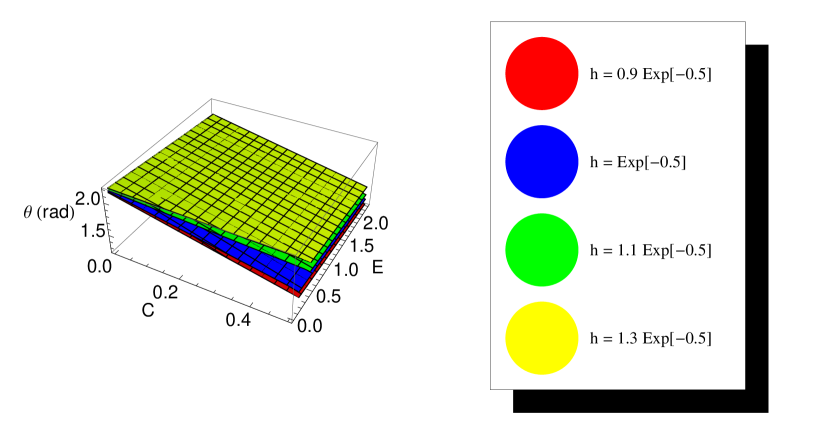
Figure 3: The apsidal angle in radians as a function of the core radius $C$ and the energy $E$. Four different angular momenta are presented in separate colours. Please see the text for more details.

Figure 3 shows the apsidal angle calculated by this method, for different values of $C$, $E$ and $h$.

$u_{c}$	$\theta$
	Lambert $W$	Numerical	Difference
	approximation
1.0	2.06310	2.06300	0.00010
1.1	2.07122	2.07116	0.00006
1.2	2.07868	2.07862	0.00006
1.3	2.08558	2.08554	0.00004
1.4	2.09201	2.09200	0.00001
1.5	2.09803	2.09797	0.00006
1.6	2.10368	2.10361	0.00007
1.7	2.10901	2.10896	0.00005
1.8	2.11405	2.11397	0.00008

Table 3: The apsidal angle as calculated for different values of $u_{c}=1/r_{c}$.

Table 3 shows how values of $u_{c}$ ranging from 1 to 1.8 yield similar apsidal angles with values near $\frac{2\pi}{3}$. For comparison, Touma & Tremaine (1997) use the epicyclic approximation for near-circular orbits to determine that their $g(\alpha,y)$ (which is twice the apsidal angle as defined here) equals $2\pi/\sqrt{2}=4.44428=2\times 2.22144$, a value close to the one arrived at here. However, a comparison with the numerically-derived result, also listed in Table 3 shows that the method proposed here is much more accurate: the two differ only in the fifth decimal place. As a comparison, we also show the apsidal angle for various values of small $e$ using the p-ellipse approximation in the column labelled ’Numerical’.

From Eq. 26, we have

$$k=\sqrt{2}{{{\left(1-\frac{e}{2}\right)}}}^{{-1}/{2}}\ \sim\ \sqrt{2}{{\left(1+\frac{e}{4}+\dots\right)}}$$ (50)

The apsidal angle is given by

$$\frac{\pi}{k}=\frac{\pi}{\sqrt{2}}{\left(1-\frac{e}{2}\right)}^{{1}/{2}}\ \sim\ \frac{\pi}{\sqrt{2}}\left(1-\frac{e}{4}-\frac{1}{32}e^{2}\dots\right)$$ (51)

It is of interest to note that the roots can be found without any approximation for $C$ in terms of the polylog function. For arbitrary $C$, one obtains from Eq. 45 an exact expression

$$-\frac{1}{C^{2}u^{2}}(\ln C^{2}-E)-\frac{1}{C^{2}u^{2}}\ln\left(1+\frac{1}{C^{2}u^{2}}\right)=\frac{h^{2}}{2C^{2}}$$ (52)

for finding the roots of $u^{2}$. Now if we define $k\equiv\ln C^{2}-E$ and $x\equiv-\frac{1}{C^{2}u^{2}}$, Eq. 52 reduces to

$$kx+x\ln(1-x) = \frac{h^{2}}{2C^{2}}$$ (53)

$$k+\ln(1-x) = \frac{h^{2}}{2C^{2}}\frac{1}{x}$$ (54)

$$k-Li_{1}(x) = \frac{h^{2}}{2C^{2}}\frac{1}{x}$$ (55)

Here Eq. 55 is the functional equation of the Polylogarithm $Li_{1}(x)=-\ln(1-x)$ Lewin (1981) and

$$x=-\frac{1}{C^{2}u^{2}}=-\frac{r^{2}}{C^{2}}$$ (56)

5 Gravitational Lensing

The use of the Lambert $W$ and the Polylogarithm functions to find the roots of equations such as Eq. 47 and 53 may have wider applicability. For example, we can use a similar approach to compute the deflection of a light ray by a logarithmic potential, useful in the context of gravitational lensing Cowling (1983); Schutz (1990); Blundell et al. (2010). Zwicky (1937) suggested that extragalactic nebulae offer a much better chance than stars for the observation of gravitational lens effects. Zwicky’s idea was that some of the massive and more concentrated nebulae may be expected to deflect light by as much as half a minute of arc. Nebulae, in contrast to stars, possess apparent dimensions which are resolvable to very great distances. Zwicky was following up on the work of Einstein (1936) on stars acting as a gravitational lens. According to Zwicky, observations on the deflection of light around nebulae may provide the most direct determination of nebular masses Smith (1936). Zwicky (1937) estimated the probability of detecting nebular galaxies which act as gravitational lenses and pointed out the possibility of ring shaped images, flux amplification and understanding the large scale structure of the universe. The lensing equation can be generalized to three dimensions and cosmological distances by correction of the redshift related distance Schneider et al. (1992).

For arbitrary $K$ one has the following expression to determine the roots in the case of light deflection for a logarithmic potential,

$$V\left(r\right)=K\ln\left(r^{2}+C^{2}\right)$$ (57)

where $K$ is a dimensionless constant and $r=\frac{1}{u}$.

For light deflection in the logarithmic potential considered, the differential equation for the given logarithmic potential is of the form

$$\frac{d^{2}u}{d\theta^{2}}+\ u=K\left(\frac{C^{2}u}{1+C^{2}u^{2}}-\frac{1}{u}\right)=\ \frac{-K}{u(1+C^{2}u^{2})}$$ (58)

The DE for small values of $C\ll 1$, reduces to

$$\therefore\frac{d^{2}u}{d\theta^{2}}+u-KC^{2}u=\frac{-K}{u}$$ (59)

In the relativistic formulation Hartle (2003) the differential equation for light deflection is

$${\left(\frac{d\theta}{du}\right)}^{2}=\frac{1}{\frac{1}{b^{2}}-u^{2}+2Mu^{3}}$$ (60)

$$\therefore u^{\prime\prime}+u=3Mu^{2}$$ (61)

where $b$ is the impact parameter.

Assuming the photon is a non-relativistic particle that travels at speed $c$ and it is far from all sources of gravitational attraction Hartle (2003), we can determine the light deflection $\Delta\theta$ produced by a logarithmic potential as

$$\Delta\theta=2\int_{0}^{u_{1}}\frac{du}{\sqrt{1-u^{2}+K\ln\left(\frac{1}{u^{2}}+C^{2}\right)}}$$ (62)

Solving for the roots of the denominator, one obtains

$$1-u^{2}+K\left[\ln\left(1+C^{2}u^{2}\right)-\ln u^{2}\right]=0$$ (63)

Solving for $K\ll 1$ by use of the Lambert $W$ function, we get

$$u^{2}=\frac{1}{\left(\frac{1}{K}-C^{2}\right)}W_{j}\left\{\left(\frac{1}{K}-C^{2}\right)e^{\frac{1}{K}}\right\}$$ (64)

where $j$ denotes the branch of the Lambert $W$ function.

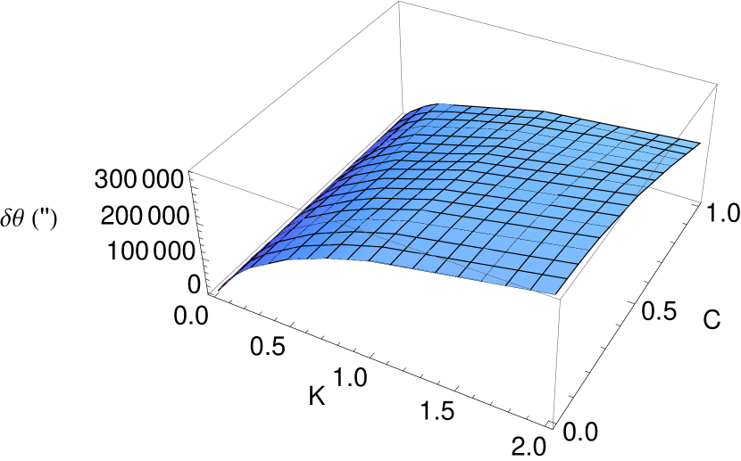
Figure 4: The deflection angle in seconds of arc as a function of $C$ and $K$. Please see the text for more details.

The deflection angle is related to the Einstein angle $\theta_{E}$ Hartle (2003) which sets the characteristic angular scale for gravitational lensing phenomena. Gravitational lensing can be used to detect mass or energy in the universe, whether visible or not. Table 4 show the deflection angle for a range of values of $K$ and $C$. Small $K$ values produce small deflections, while smaller values of $C$ produce larger ones, though with a weaker dependence. Figure 4 shows the variation graphically.

$K$	$C$	$\Delta\theta$
	1.0	0.00444
$10^{-8}$	0.5	0.00703
	0.0005	0.00491
	1.0	2256.33
0.005	0.5	2861.51
	0.0005	3202.15
	1.0	69 637.4
0.25	0.5	95 986.9
	0.0005	109 909
	1.0	104 102
0.5	0.5	150 674
	0.0005	173 731
	1.0	142 042
1	0.5	218 327
	0.0005	251 802
	1.0	178 640
2	0.5	292 967
	0.0005	334 185

Table 4: The deflection angle $\Delta\theta$ (in seconds of arc) as a function of $k$ and $C$.

Analogous calculations can be done for time delay in light signals due to lensing galaxies Ohanian & Ruffini (1994). Intensity fluctuations caused by lumpy dark matter may provide direct observational existence for it. It is worth noting that the entire analysis can not only be done for the purely radial logarithmic potential, but also for the Eq. 1 of the logarithmic potential, by considering the $x$ and $y$ components separately as was done for the gravitational potential Bourassa & Kantowski (1975).

6 Conclusions

We have revisited and expanded the work of Contopoulos & Seimenis (1990) on orbits within a logarithmic potential. We did a comprehensive review of the Prendergast method used by CS. We performed an analytic and numerical study of the matrix: $C_{-3}$, $C_{-2}$, $C_{-1}$, $C_{0}$, $C_{1}$, $C_{2}$ that resulted in eighteen equations for the six coefficients for the orbital Fourier type series solution for values of $U$ ranging from 0.1 to 1 that gave the unperturbed as well as perturbed solutions with better precision. The apsidal angle for the case of galactic orbits for a planar scale-free spherical logarithmic potential was obtained from the p-ellipse solution of the orbital differential equation and also the Lambert $W$. Both the Lambert $W$ and the Polylogarithm functions may have applications in problems involving exponential and/or logarithmic potentials such as gravitational lensing.

The Prendergast method, although not used as widely as others, has been quite useful in our analysis in Sections 2 and 3., and is likely to prove useful in the study of many types of galactic potentials.

Gravitational lensing can be used to detect mass in the universe, whether dark or visible Hartle (2003); Narlikar (2010). In general relativity, all energy curves spacetime, and a constant vacuum energy produces a detectable curvature. Gravity may prove a useful tool for detecting and studying dark energy. The lensing due to the gravitational field of a black hole of background stars and galaxies Thorne (1994) can be significant and the effects of a logarithmic potential warrant further study in this connection.

7 Acknowledgements

We gratefully acknowledge discussions with Dr. Seimenis during our work. We thank Curt Struck (Iowa State University) for sending earlier work on p-ellipse orbits. We also thank the anonymous referee for a stimulating review of our manuscript. SRV gratefully acknowledges research funding from King’s University College at the University of Western Ontario. This work was supported in part by the Natural Sciences and Engineering Research Council of Canada (NSERC).

Appendix A Perturbed equations

The following are the equations for Equation 16

$${\it S_{11}}={\it E_{6}}-{U}^{2}{\it E_{1}}\left(\nu-3\right)^{2}{\omega}^{2};$$

$${\it S_{13}}=0.5{\it E_{7}}-0.5{U}^{2}{\it E_{2}}{\omega}^{2}\left(\nu-1\right)^{2}-0.5{U}^{2}{\it E_{4}}\omega\left(\nu-1\right);$$

$${\it S_{15}}=0.5{\it E_{8}}-0.5{U}^{2}{\it E_{3}}{\omega}^{2}\left(\nu+1\right)^{2}-0.5{U}^{2}{\it E_{5}}\omega\left(\nu+1\right);$$

$${\it S_{22}}={\it E_{6}}-{U}^{2}{\it E_{1}}\left(\nu-2\right)^{2}{\omega}^{2};$$

$${\it S_{24}}=0.5{\it E_{7}}-0.5{U}^{2}{\it E_{2}}{\omega}^{2}{\nu}^{2}-0.5{U}^{2}{\it E_{4}}\omega\nu;$$

$${\it S_{26}}=0.5{\it E_{8}}-0.5{U}^{2}{\it E_{3}}{\omega}^{2}\left(\nu+2\right)^{2}-0.5{U}^{2}{\it E_{5}}\omega\left(\nu+2\right);$$

$${\it S_{31}}=0.5{\it E_{7}}-0.5{U}^{2}{\it E_{2}}{\omega}^{2}\left(\nu-3\right)^{2}+0.5{U}^{2}{\it E_{4}}\omega\left(\nu-3\right);$$

$${\it S_{33}}={\it E_{6}}-{U}^{2}{\it E_{1}}\left(\nu-1\right)^{2}{\omega}^{2};$$

$${\it S_{35}}=0.5{\it E_{7}}-0.5{U}^{2}{\it E_{2}}{\omega}^{2}\left(\nu+1\right)^{2}-0.5{U}^{2}{\it E_{4}}\omega\left(\nu+1\right);$$

$${\it S_{42}}=0.5{\it E_{7}}-0.5{U}^{2}{\it E_{2}}{\omega}^{2}\left(\nu-2\right)^{2}+0.5{U}^{2}{\it E_{4}}\omega\left(\nu-2\right);$$

$${\it S_{44}}={\it E_{6}}-{U}^{2}{\it E_{1}}{\omega}^{2}{\nu}^{2};$$

$${\it S_{46}}=0.5{\it E_{7}}-0.5{U}^{2}{\it E_{2}}{\omega}^{2}\left(\nu+2\right)^{2}-0.5{U}^{2}{\it E_{4}}\omega\left(\nu+2\right);$$

$${\it S_{51}}=0.5{\it E_{8}}-0.5{U}^{2}{\it E_{3}}{\omega}^{2}\left(\nu-3\right)^{2}+0.5{U}^{2}{\it E_{5}}\omega\left(\nu-3\right);$$

$${\it S_{53}}=0.5{\it E_{7}}-0.5{U}^{2}{\it E_{2}}{\omega}^{2}\left(\nu-1\right)^{2}+0.5{U}^{2}{\it E_{4}}\omega\left(\nu-1\right);$$

$${\it S_{55}}={\it E_{6}}-{U}^{2}{\it E_{1}}\left(\nu+1\right)^{2}{\omega}^{2};$$

$${\it S_{62}}=0.5{\it E_{8}}-0.5{U}^{2}{\it E_{3}}{\omega}^{2}\left(\nu-2\right)^{2}+0.5{U}^{2}{\it E_{5}}\omega\left(\nu-2\right);$$

$${\it S_{64}}=0.5{\it E_{7}}-0.5{U}^{2}{\it E_{2}}{\omega}^{2}{\nu}^{2}+0.5{U}^{2}{\it E_{4}}\omega\nu;$$

$${\it S_{66}}={\it E_{6}}-{U}^{2}{\it E_{1}}\left(\nu+2\right)^{2}{\omega}^{2}.$$

In $S_{22}$ the bracketed term $(\nu-2)$ has been corrected from the original form with $(\nu-1)$ in CS.

The corresponding $E$ values are

$${\it E_{1}}={C}^{2}\left(0.375{B}^{4}+3{B}^{2}+1\right)+0.5{A}^{2}\left(0.5{B}^{2}+B+1\right);$$

$${\it E_{2}}={C}^{2}\left(3{B}^{3}+4B\right)+{A}^{2}\left(0.375{B}^{2}+B+0.5\right);$$

$${\it E_{3}}={C}^{2}\left(0.5{B}^{4}+3{B}^{2}\right)+0.5{A}^{2}\left(0.5{B}^{2}+B\right);$$

$${\it E_{4}}=2\omega B\left({A}^{2}+2{C}^{2}+{C}^{2}{B}^{2}\right)+\omega{B}^{2}\left(0.5{A}^{2}+2{C}^{2}B\right)-\omega{B}^{3}{C}^{2};$$

$${\it E_{5}}=\omega{B}^{2}\left({A}^{2}+2{C}^{2}+{C}^{2}{B}^{2}\right)+\omega B\left({A}^{2}+4{C}^{2}B\right);$$

$${\it E_{6}}={U}^{2}{\omega}^{2}B\left({A}^{2}+3{A}^{2}B+10{C}^{2}B+2.5{C}^{2}{B}^{3}\right)+0.75{B}^{4}+6{B}^{2}+2;$$

$${\it E_{7}}={U}^{2}{\omega}^{2}B\left(2{A}^{2}+2.5{A}^{2}B+4{C}^{2}+13{C}^{2}{B}^{2}\right)+6{B}^{3}+8B;$$

$${\it E_{8}}={U}^{2}{\omega}^{2}B\left({A}^{2}-{A}^{2}B+2{C}^{2}B+2{C}^{2}{B}^{3}\right)+{B}^{4}+6{B}^{2}.$$

In $E_{4}$ the term with $0.5A^{2}$ has been corrected from its original form of $0.5A$ in CS.

References

- Belmonte et al. (2007) Belmonte C., Boccaletti D., Pucacco G., 2007, ApJ, 669, 202
- Binney & Spergel (1982) Binney J., Spergel D., 1982, ApJ, 252, 308
- Binney & Tremaine (1987) Binney J., Tremaine S., 1987, Galactic Dynamics. Princeton University Press, Princeton
- Blundell et al. (2010) Blundell K. M., Schechter P. L., Morgan N. D., Jarvis M. J., Rawlings S., Tonry J. L., 2010, ApJ, 723, 1319
- Bourassa & Kantowski (1975) Bourassa R. R., Kantowski R., 1975, ApJ, 195, 13
- Chandrasekhar (1983) Chandrasekhar S., 1983, The Mathematical Theory of Black Holes. Claredon Press, Oxford
- Contopoulos & Seimenis (1990) Contopoulos G., Seimenis J., 1990, A&A, 227, 49
- Cowling (1983) Cowling S., 1983, PhD thesis, University Colledge, Cardiff
- Einstein (1936) Einstein A., 1936, Science, 84, 506
- Evans (1927) Evans G. C., 1927, The Logarithmic Potential: Discontinuous Dirichlet and Neumann Problems. American Mathematical Society, Providence, Rhode Island
- Evans (1993) Evans N. W., 1993, MNRAS, 260, 191
- Floquet (1883) Floquet G., 1883, Ann. Ec. Norm Suppl. (2), 12, 47
- Gerhard & Binney (1985) Gerhard O. E., Binney J., 1985, MNRAS, 216, 467
- Hagihara (1931) Hagihara Y., 1931, Japanese Journal of Astronomy and Geophysics, vol. 8, p. 67-176 (1931), 8, 67
- Hartle (2003) Hartle J. B., 2003, Gravity: An Introduction to Einstein’s General Relativity. Addison-Wesley, San Franscisco
- Kamke (1943) Kamke E., 1943, Differential Gleichungen Losungsmethoden ung Losungen. Gesst & Portig, Leibzig
- Karanis & Caranicolas (2001) Karanis G. I., Caranicolas N. D., 2001, A&A, 367, 443
- Lees & Schwarzschild (1992) Lees J. F., Schwarzschild M., 1992, ApJ, 384, 491
- Lewin (1981) Lewin L., 1981, Polylogarithms and Associated Functions. North-Holland, Amsterdam
- Magnenat (1982) Magnenat P., 1982, A&A, 108, 89
- Miralda-Escude & Schwarzschild (1989) Miralda-Escude J., Schwarzschild M., 1989, ApJ, 339, 752
- Murray & Dermott (1999) Murray C., Dermott S., 1999, Solar System Dynamics. Cambridge University Press, Cambridge
- Narlikar (2010) Narlikar J. V., 2010, An Introduction to Relativity. Cambridge University Press, Cambridge
- Ohanian & Ruffini (1994) Ohanian H. C., Ruffini R., 1994, Gravitation and Spacetime. Norton, New York
- Pfenniger & de Zeeuw (1989) Pfenniger D., de Zeeuw T., 1989, in D. Merritt ed., Dynamics of Dense Stellar Systems Central density cusps and triaxiality. pp 81–87
- Prendergast (1982) Prendergast K., 1982, in David Chudnovsky G., eds, Lecture Notes in Mathematics 925: The Riemann Problem, Complete Integrability and Arithmetic Applications Rational approximation for non-linear ordinary differential equations. Springer, New York
- Pucacco et al. (2008) Pucacco G., Boccaletti D., Belmonte C., 2008, A&A, 489, 1055
- Quigg & Rosner (1977) Quigg C., Rosner J. L., 1977, Phys. Lett. B, 71, 153
- Richstone (1980) Richstone D. O., 1980, ApJ, 238, 103
- Richstone (1982) Richstone D. O., 1982, ApJ, 252, 496
- Sachdev (1991) Sachdev P. L., 1991, Nonlinear Ordinary Differential Equations and Their Applications. Cambridge University Press, Cambridge
- Schneider et al. (1992) Schneider P., Ehlers J., Falco E. E., 1992, Gravitational Lenses. Springer, Berlin
- Schutz (1990) Schutz B. F., 1990, A First Course in General Relativity. Cambridge University Press, Cambridge
- Smith (1936) Smith S., 1936, ApJ, 83, 23
- Struck (2006) Struck C., 2006, AJ, 131, 1347
- Thorne (1994) Thorne K. S., 1994, Black Holes and Time Warps: Einstein’s Outrageous Legacy. Norton, New York
- Touma & Tremaine (1997) Touma J., Tremaine S., 1997, MNRAS, 292, 905
- Valluri et al. (2000) Valluri S. R., Jeffrey D. J., Corless R. M., 2000, Canadian Journal of Physics, 78, 823
- Valluri et al. (2005) Valluri S. R., Yu P., Smith G. E., Wiegert P. A., 2005, MNRAS, 358, 1273
- Zwicky (1937) Zwicky F., 1937, Phys. Rev. Lett., 51, 290