Invariants of closed braids via counting surfaces

Abstract.

A Gauss diagram is a simple, combinatorial way to present a link. It is known that any Vassiliev invariant may be obtained from a Gauss diagram formula that involves counting subdiagrams of certain combinatorial types. In this paper we present simple formulas for an infinite family of invariants in terms of counting surfaces of a certain genus and number of boundary components in a Gauss diagram associated with a closed braid. We then identify the resulting invariants with partial derivatives of the HOMFLY-PT polynomial.

1. Introduction.

In this paper we consider link invariants arising from the HOMFLY-PT polynomials. The HOMFLY-PT polynomial $P(L)$ is an invariant of an oriented link $L$ (see e.g. [6], [8], [11], [15]). It is a Laurent polynomial in two variables $a$ and $z$, which satisfies the following skein relation:

$$aP\left(\raisebox{-11.38109pt}{\includegraphics[width=28.45274pt]{L+.eps}}\right)-a^{-1}P\left(\raisebox{-11.38109pt}{\includegraphics[width=28.45274pt]{L-.eps}}\right)=zP\left(\raisebox{-11.38109pt}{\includegraphics[width=28.45274pt]{L0.eps}}\right).$$

The HOMFLY-PT polynomial is normalized in the following way. If $O_{r}$ is an $r$-component unlink, then $P(O_{r})=\left(\frac{a-a^{-1}}{z}\right)^{r-1}$. The Conway polynomial $\nabla$ may be defined as $\nabla(L):=P(L)|_{a=1}$. This polynomial is a renormalized version of the Alexander polynomial (see e.g. [5], [10]). All coefficients of $\nabla$ are finite type or Vassiliev invariants.

One of the mainstream and simplest techniques for producing Vassiliev invariants are so-called Gauss diagram formulas (see [7], [14]). These formulas generalize the calculation of a linking number by counting subdiagrams of special geometric-combinatorial types with signs and weights in a given link diagram.

Until recently, explicit formulas of this type were known only for few invariants of low degrees. The situation has changed with works of Chmutov-Khoury-Rossi [3] and Chmutov-Polyak [4]. In [3] Chmutov-Khoury-Rossi presented an infinite family of Gauss diagram formulas for all coefficients of $\nabla(L)$, where $L$ is a knot or a two-component link. Each formula for the coefficient $c_{n}$ of $z^{n}$ is related to a certain count of orientable surfaces of a certain genus, and with one boundary component. The genus depends only on $n$ and the number of the components of $L$.

In a recent paper [1] the author showed that the $n$-th coefficient of the polynomial $zP^{(1)}_{a}(L)|_{a=1}$, where $P^{(k)}_{a}(L)|_{a=1}$ is the $k$-th partial derivative of the HOMFLY-PT polynomial $P$ w.r.t. the variable $a$ evaluated at $a=1$, can be obtained by a certain count of orientable surfaces of some genus with one and two boundary components. And again the genus depends only on $n$ and the number of the components of $L$.

This leads to a natural question: how to produce link invariants by counting orientable surfaces with an arbitrary number of boundary components? In this paper we are going to show that the $n$-th coefficient of the polynomial $z^{k}P^{(k)}_{a}(L)|_{a=1}$ can be obtained by a similar count of orientable surfaces of a certain genus with one up to k+1 boundary components, see Theorem 4.1.

Plan of the paper. In Section 2 we review Gauss diagrams and Gauss diagram formulas. We define a notion of multi-based arrow diagrams and formulate our main result in terms of Gauss diagrams. In Section 3 we show that our invariant satisfies certain skein relation. In Section 4 we give a proof of our main Theorem 4.1, and give an example. Section 5 is used for final remarks.

Acknowledgments. The author would like to thank Michael Polyak and Hao Wu for helpful conversations. We would like to thank the anonymous referee for careful reading of our paper and for his/her helpful comments and remarks. Part of this work has been done during the author’s stay in Mathematisches Forschungsinstitut Oberwolfach. The author wishes to express his gratitude to the institute. He was supported by the Oberwolfach Leibniz fellowship.

2. Gauss diagrams and arrow diagrams

In this section we recall a notion of Gauss diagrams, arrow diagrams and Gauss diagram formulas. We then define a special type of arrow diagrams which will be used to define Gauss diagram formulas for coefficients of polynomials derived from the HOMFLY-PT polynomial.

2.1. Gauss diagrams of links

Gauss diagrams (see e.g. [7], [14]) provide a simple combinatorial way to encode oriented links.

Definition 2.1.

Given a link diagram $D$, consider a collection of oriented circles parameterizing it. Unite two preimages of every crossing of $D$ in a pair and connect them by an arrow, pointing from the overpassing preimage to the underpassing one. To each arrow we assign a sign (local writhe) of the corresponding crossing. The result is called the Gauss diagram $G$ corresponding to $D$.

We consider Gauss diagrams up to an orientation-preserving diffeomorphisms of the circles. In figures we will always draw circles of the Gauss diagram with a counter-clockwise orientation. A classical link can be uniquely reconstructed from the corresponding Gauss diagram [7].

Example 2.2.

Diagrams of the trefoil knot and the Hopf link, together with the corresponding Gauss diagrams, are shown in the following picture.

            

Two Gauss diagrams represent isotopic links if and only if they are related by a finite number of Reidemeister moves for Gauss diagrams shown in Figure 1, where $\varepsilon=\pm 1$. See e.g. [2, 12, 13].

$$\Omega_{1}:\quad\raisebox{-19.91692pt}{\includegraphics[width=85.35826pt]{reidemeister1.eps}}\quad\quad\quad\Omega_{2}:\quad\raisebox{-19.91692pt}{\includegraphics[width=128.0374pt]{reidemeister2.eps}}$$

$$\Omega_{3}:\quad\raisebox{-22.76219pt}{\includegraphics[width=184.9429pt]{reidemeister3.eps}}$$

Figure 1. Reidemeister moves of Gauss diagrams.

2.2. Gauss diagrams of closed braids

Recall that the Artin braid group $B_{m}$ on $m$ strings has the following presentation:

$$B_{m}=\langle\sigma_{1},\ldots,\sigma_{m-1}|\hskip 5.69054pt\sigma_{i}\sigma_{j}=\sigma_{j}\sigma_{i},\hskip 2.84526pt|i-j|\geq 2;\hskip 5.69054pt\sigma_{i}\sigma_{i+1}\sigma_{i}=\sigma_{i+1}\sigma_{i}\sigma_{i+1}\rangle,$$

where each generator $\sigma_{i}$ is shown in Figure 2a.

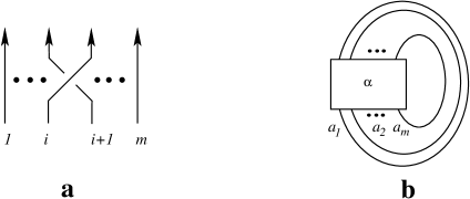
Figure 2. Artin generator $\sigma_{i}$ and a closure of a braid $\alpha$.

Let $w$ be a word on $m$ strings in generators $\sigma_{1}^{\pm 1},\ldots,\sigma_{m-1}^{\pm 1}$. We take the corresponding "geometric word", connect it opposite ends by nonintersecting curves as shown in Figure 2b and get an oriented link diagram $D$. Let us remove from $D$ a small neighborhood around each intersection point. We define an arc in $D$ to be a connected component of the resulting graph, and label the arcs of $D$ shown in Figure 2b by letters $a_{1},...,a_{m}$. Two words $w$ and $w^{\prime}$ on $m$ strings represent the same element in $B_{m}$ up to conjugation, if and only if the associated diagrams $D$ and $D^{\prime}$ can be obtained one from another by a finite sequence of moves shown in Figure 3, see e.g. [9]. Note that the moves shown in Figure 3 may also involve labeled arcs.

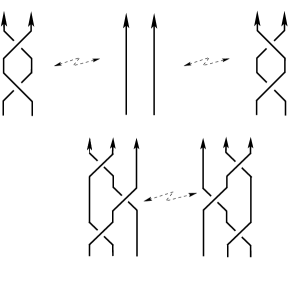
Figure 3. Reidemeister moves of braid diagrams.

$$\Omega_{1}:\hskip 51.21495pt\raisebox{-19.91692pt}{\includegraphics[width=241.84842pt]{B-R1-move.eps}}$$

$$\Omega_{2}:\hskip 28.45274pt\raisebox{-99.58464pt}{\includegraphics[width=227.62204pt]{B-R2-move.eps}}$$

$$\Omega_{3}:\hskip 56.9055pt\raisebox{-22.76219pt}{\includegraphics[width=199.16928pt]{reidemeister3.eps}}$$

Figure 4. Reidemeister moves of braid Gauss diagrams. The move $\Omega_{2}$ may involve arcs labeled by $a_{i}$ and $a_{j}$. In this case we require that $|i-j|=1$. The move $\Omega_{3}$ may involve labeled arcs as well, i.e. two corresponding arcs may be labeled by some $a_{i}$.

Let $D$ be any diagram associated with a braid $\alpha\in B_{m}$. A corresponding braid Gauss diagram $G_{m}$ is a Gauss diagram $G$ together with the corresponding arcs labeled by letters $a_{1},...,a_{m}$, where an arc in $G$ is a connected component of the complement of all arrows in $G$. Similarly to the case of Gauss diagrams, two braid Gauss diagrams represent isotopic links if and only if they are related by a finite number of moves shown in Figure 4.

Definition 2.3.

Let $k\geq 1$ be any integer and $G_{m}$ a braid Gauss diagram associated with a braid $\alpha\in B_{m}$. A colored braid Gauss diagram $G_{k,m}$ is a diagram $G$ together with the following assignment of $k$ base points $*_{1},...,*_{k}$ and $m-k$ natural numbers between $1$ and $k$ to the arcs labeled by letters $a_{1},...,a_{m}$:

• For each $1\leq i\leq k$ there exists exactly one arc $a_{j}$ such that the base point $*_{i}$ is placed on this arc, and the arc $a_{1}$ always contains basepoint $*_{1}$.

• Let $1\leq i_{1}<i_{2}\leq k$. If $*_{i_{1}}$ and $*_{i_{2}}$ are placed on arcs $a_{j_{1}}$ and $a_{j_{2}}$, then $j_{1}<j_{2}$, i.e. the assignment of base points is in ascending order.

• After we placed base points $*_{1},...,*_{k}$ on arcs $a_{j_{1}},...,a_{j_{k}}$, let $a_{j}$ be a non-based arc. Denote by $j_{l}$ the maximal number from the set $\{j_{1},...,j_{k}\}$ such that $j>j_{l}$. Now, to arc $a_{j}$ we assign exactly one number from the set $\{1,...,l\}$.

Let us give an example of a colored braid Gauss diagram, in case when $k=3$, since the above definition seems to be complicated. In Figure 5 we show a braid diagram for $\sigma_{1}\sigma_{2}\sigma_{3}\in B_{4}$, the corresponding braid Gauss diagram and an associated colored braid Gauss diagram $G_{3,4}$.

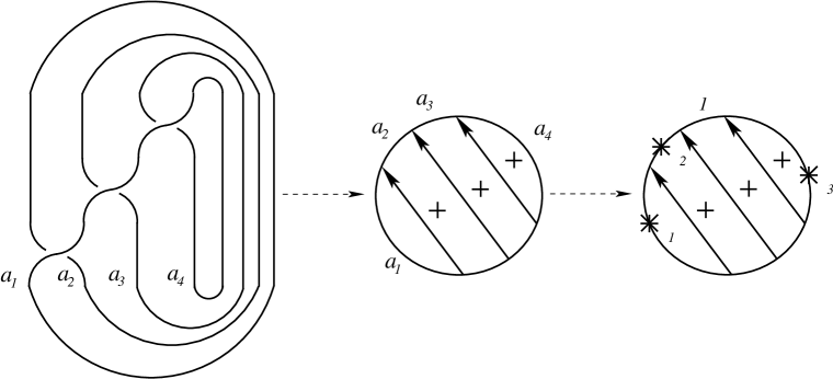
Figure 5. Braid diagram on the left, the corresponding braid Gauss diagram in the middle and an associated colored braid Gauss diagram $G_{3,4}$ on the right. A base point $*_{1}$ is placed on arc labeled by $a_{1}$, a base point $*_{2}$ is placed on arc labeled by $a_{2}$, a base point $*_{3}$ is placed on arc labeled by $a_{4}$, and so the assignment of the base points is in ascending order. Now we have to place a number from $\{1,2,3\}$ on arc labeled by $a_{3}$. Since in this case $j_{1}=1$, $j_{2}=2$ and $j_{3}=4$, we can place any number from $\{1,2\}$ on arc labeled by $a_{3}$. In this picture we placed number 1.

We denote by $\mathfrak{G}_{k,m}$ a set of all colored braid Gauss diagrams associated with $k$ and $G_{m}$. Note that $\mathfrak{G}_{k,m}$ is empty whenever $k>m$.

2.3. Arrow diagrams and the corresponding surfaces

An arrow diagram is a modification of a notion of a Gauss diagram, i.e. it consists of a number of oriented circles with several arrows connecting pairs of distinct points on them, see Figure 6. An arrow diagram is based if a base point is placed on an arc of $A$. We consider these diagrams up to orientation-preserving diffeomorphisms of the circles.

Figure 6. Based connected arrow diagrams.

Given an arrow diagram $A$, we define an oriented surface $\Sigma(A)$ as follows. Firstly, replace each circle of $A$ with an oriented disk bounding this circle. Secondly, glue $1$-handles to boundaries of these disks using each arrow as a core of an untwisted ribbon, such that the ribbons do not intersect in $\mathbb{R}^{3}$. See Figures 7 and 8.

Figure 7. Constructing a surface from an arrow diagram.

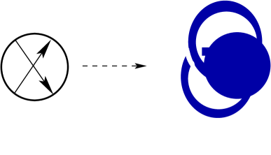
Figure 8. Arrow diagram with 2 arrows and a corresponding surface, which is homeomorphic to the torus with one boundary component.

Definition 2.4.

By the genus and the number of boundary components of an arrow diagram $A$ we mean the genus and the number of boundary components of $\Sigma(A)$. An arrow in $A$ is called separating, if the boundary of the corresponding ribbon belongs to different boundary components of $\Sigma(A)$.

Remark 2.5.

Let $A$ be an arrow diagram with $n$ arrows and $r$ circles. Then the Euler characteristic $\chi$ of $\Sigma(A)$ equals to $\chi(\Sigma(A))=r-n$. If $A$ is connected, $n\geq r-1$. If $A$ has odd number of boundary components, $n\neq r(\rm{mod}2)$, otherwise $n=r(\rm{mod}2)$.

Example 2.6.

The arrow diagram with one circle in Figure 6 is of genus one, while the other arrow diagram in the same figure is of genus zero. Both of them have one boundary component.

Definition 2.7.

An arrow diagram $A$ with $k$ boundary components is multibased if $k$ base points $*_{1},...,*_{k}$ are placed on $k$ different arcs of $A$, such that each arc belongs to a different boundary component of $A$, see Figure 9. Let $1\leq j\leq k$. We say that a boundary component of $A$ is called $j$-th boundary component if there exists an arc, which belongs to this component, with a base point $*_{j}$ on it.

Figure 9. Multibased arrow diagram with 3 boundary components.

2.4. Gauss diagram formulas

M. Polyak and O. Viro suggested [14] the following approach to compute link invariants using Gauss diagrams.

Definition 2.8.

Let $A$ be a based arrow diagram with $r$ circles and let $G$ be a based Gauss diagram of an $r$-component oriented link. A homomorphism $\phi:A\rightarrow G$ is an orientation preserving homeomorphism between each circle of $A$ and each circle of $G$, which maps the base point of $A$ to the base point of $G$ and induces an injective map of arrows of $A$ to the arrows of $G$. The set of arrows in $\operatorname{Im}(\phi)$ is called a state of $G$ induced by $\phi$ and is denoted by $S(\phi)$. The sign of $\phi$ is defined as $\operatorname{sign}(\phi)=\prod_{\alpha\in S(\phi)}sign(\alpha)$. A set of all homomorphisms $\phi:A\to G$ is denoted by $\operatorname{Hom}(A,G)$.

Note that since the circles of $A$ are mapped to circles of $G$, a state $S$ of $G$ determines both the arrow diagram $A$ and the map $\phi:A\to G$ with $S=S(\phi)$.

Definition 2.9.

A pairing between an arrow diagram $A$ and $G$ is defined by

$$\langle A,G\rangle=\sum_{\phi\in\operatorname{Hom}(A,G)}\operatorname{sign}(\phi).$$

We set $\langle A,G\rangle=0$, whenever $A$ and $G$ have different number of circles.

For an arbitrary arrow diagram $A$ the pairing $\langle A,G\rangle$ does not represent a link invariant, i.e. it depends on the choice of a Gauss diagram of a link. However, for some special linear combinations of arrow diagrams the result is independent of the choice of $G$. Using a slightly modified definition of arrow diagrams Goussarov, Polyak and Viro showed in [7] that each real-valued Vassiliev invariant of knots may be obtained this way. In other words, they showed that each real-valued Vassiliev invariant of knots may be computed as a certain count with weights of subdiagrams of a based Gauss diagram. For example, all coefficients of the Conway polynomial $\nabla$ may be obtained using suitable combinations of arrow diagrams. More precisely, in [3] it was shown that the coefficient $c_{n}$ of $z_{n}$ in $\nabla$ can be obtained by a certain count of arrow diagrams with one boundary component and certain genus, where the genus depends only on $n$ and the number of circles in $G$.

In [1] we showed that the $n$-th coefficient of the polynomial $zP^{(1)}_{a}|_{a=1}$ can be obtained by a certain count of arrow diagrams with one and two boundary components and certain genus. And again the genus depends only on $n$ and the number of circles in $G$. In what follows we are going to show that, in case when $G$ is a braid Gauss diagram of a link, the $n$-th coefficient of the polynomial $z^{k}P^{(k)}_{a}|_{a=1}$ can be obtained by a similar count of arrow diagrams with one up to k+1 boundary components and a certain genus. Hence we need to adopt Definition 2.8 to the case of multi-based arrow diagrams and colored braid Gauss diagrams.

Definition 2.10.

Let $A$ be a multi-based arrow diagram with $r$ circles and $k$ boundary components and let $G_{k,m}$ be a colored braid Gauss diagram of an $r$-component closed braid on $m$ strings. A homomorphism $\phi:A\rightarrow G_{k,m}$ is an orientation preserving homeomorphism between each circle of $A$ and each circle of $G_{k,m}$, which maps each base point $*_{i}$ of $A$ to each base point $*_{i}$ of $G_{k,m}$ and induces an injective map of arrows of $A$ to the arrows of $G_{k,m}$. In addition we require that if a non-based arc $a$ of $G_{k,m}$ is labeled by some $j$, then $a$ is an image of some arc which lies in the $j$-th boundary component of $A$. The notion of state and pairing is defined as before.

2.5. Descending arrow diagrams

In this subsection we define a special type of multi-based arrow diagrams.

Definition 2.11.

Let $A$ be a multi-based arrow diagram with $k$ boundary components. As we go along the first boundary component of $\Sigma(A)$ starting from the base point $*_{1}$, we pass on the boundary of each ribbon once or twice. Then we continue to go along the second boundary component of $\Sigma(A)$ starting from the base point $*_{2}$ and so on until we pass all boundary components of $\Sigma(A)$. Arrow diagram $A$ is descending if we pass each ribbon of $\Sigma(A)$ first time in the direction of its core arrow.

Remark 2.12.

In order to define the notion of descending arrow diagrams we used the fact that all arrow diagrams are multi-based. The position of base points in an arrow diagram is essential to define an order of the passage.

From now on we will work only with multi-based arrow diagrams.

Example 2.13.

Arrow diagram with two boundary components in Figure 10a is descending and arrow diagram with three boundary components in Figure 10b is not descending.

Figure 10. Descending and non-descending arrow diagrams.

Denote by $\mathcal{D}_{n,k}$ the set of all descending arrow diagrams with $n$ arrows and $k$ boundary components.

Example 2.14.

The set $\mathcal{D}_{2,1}$ is presented below.

$$\mathcal{D}_{2,1}:=\quad\raisebox{-11.38109pt}{\includegraphics[width=227.62204pt]{D21.eps}}$$

Let $G_{m}$ be any braid Gauss diagram. We denote by $w(G_{m})$ the writhe of $G_{m}$, i.e. the sum of signs of all arrows in $G_{m}$. For each pair of natural numbers $j,k$ denote by

$$f_{j}^{(k)}(G_{m}):=\left(a^{-m-w(G_{m})+1}(a^{2}-1)^{j-1}\right)^{(k-1)}|_{a=1}.$$

Let $G\in\mathfrak{G}_{k,m}$. A state $S(\phi)$ corresponding to $\phi:A\to G$ for a descending diagram $A$ with $k$ boundary components will be also called descending.

Definition 2.15.

For a pair $k,j$ such that $1\leq j\leq k$ set

$$D_{n,k,j}(G_{m}):=\sum_{G\in\mathfrak{G}_{j,m}}\sum_{A\in\mathcal{D}_{n+j-k,j}}\langle A,G\rangle$$

and denote by

$$D_{n,k}(G_{m}):=\sum_{j=1}^{k}f_{j}^{(k)}(G_{m})D_{n,k,j}(G_{m}).$$

Define the following polynomial:

$$P_{k}(G_{m}):=\sum_{n=0}^{\infty}D_{n,k}(G_{m})z^{n}.$$

Remark 2.16.

Let $G_{m}$ be any braid Gauss diagram of a link $L$. Note that if $k=1$, then $f_{1}^{(1)}(G_{m})=1$ and $D_{n,1}(G_{m})=D_{n,1,1}(G_{m})$ is exactly the sum with signs of all descending arrow diagrams with one base point and with one boundary component inside $G_{m}$. It follows by Theorem of Chmutov-Khoury-Rossi [3] that $D_{n,1}(G_{m})$ is the $n$-th coefficient $c_{n}(L)$ of the Conway polynomial $\nabla(L)$. Hence $P_{1}(G_{m})$ is nothing but $\nabla(L)$.

3. Skein relation

In this section we show that each $D_{n,k,j}(G_{m})$ satisfies Conway skein relation for each $n$ and $1\leq j\leq k$. The fact that $D_{n,1,1}(G_{m})$ satisfies Conway skein relation was proved in [1, 3], i.e.

Figure 11. A Conway triple of Gauss diagrams.

Theorem 3.1.

[1, 3] Let $G_{m,+}$, $G_{m,-}$ and $G_{m,0}$ be braid Gauss diagrams which differ only in the fragment shown in Figure 11. Then

(1) $$P_{1}(G_{m,+})-P_{1}(G_{m,-})=zP_{1}(G_{m,0}).$$

Here we define a notion of a separating state. This notion will be used in the proof of Theorem 3.7.

Figure 12. Descending labeling.

Definition 3.2.

Let $G_{m}$ be a braid Gauss diagram and $G\in\mathfrak{G}_{k,m}$. A descending separating state $S$ of $G$ is a state $S$ of $G$, together with a labeling of all arcs of $G$ by numbers from $1$ to $k$ such that:

• An arc with a basepoint $*_{i}$ is labeled by $i$.

• Each arc near $\alpha\in S$ is labeled as in Figure 12a.

• Each arc near $\alpha\notin S$ is labeled as in Figure 12b.

Let $G\in\mathfrak{G}_{k,m}$. Then every descending separating state $S$ in $G$ defines a new Gauss diagram $G_{S}$ with labeled circles as follows:
We smooth each arrow in $G$ which belongs to $S$, as shown in Figure 13, and denote resulting smoothed Gauss diagram by $G_{S}$. Each circle in $G_{S}$ is labeled by $i$, if it contains an arc labeled by $i$.

Figure 13. Smoothing of an arrow.

Now we return to arrow diagrams. Let $A\in\mathcal{D}_{n,k}$. We denote by $\sigma(A)$ the set of separating arrows in $A$ and label the arcs of circles in $A$ by $i$ if the corresponding arc belongs to the $i$-th boundary component of $\Sigma(A)$. Note that for each $G\in\mathfrak{G}_{k,m}$ the homomorphism $\phi:A\rightarrow G$ induces a descending separating state $S$ of $G$, by taking $S=\phi(\sigma(A))$ and labeling each arc of $G$ by the same label as the corresponding arc of $A$.

Definition 3.3.

Let $S$ be a descending separating state of $G\in\mathfrak{G}_{k,m}$, $A\in\mathcal{D}_{n,k}$, and $\phi:A\rightarrow G$. We say that $\phi$ is $S$-admissible, if a descending separating state induced by $\phi$ coincides with $S$.

Definition 3.4.

Let $S$ be a descending separating state of $G\in\mathfrak{G}_{k,m}$, and $A\in\mathcal{D}_{n,k}$. We define an $S$-pairing $\langle A,G\rangle_{S}$ by:

$$\langle A,G\rangle_{S}:=\sum\limits_{\phi:A\rightarrow G}\operatorname{sign}(\phi),$$

where the summation is over all $S$-admissible $\phi:A\rightarrow G$. We set

$$D_{n,k}(G)_{S}:=\sum_{A\in\mathcal{D}_{n,k}}\langle A,G\rangle_{S}.$$

Every descending separating state $S$ of $G$ defines Gauss diagrams $\{G^{i}_{S}\}_{i=1}^{k}$ as follows: $G^{i}_{S}$ consists of all circles of $G_{S}$ labeled by $i$, and its arrows are arrows of $G$ with both ends on these circles. All arrows with ends on circles of $G_{S}$ with different labels are removed. The base point of $G^{i}_{S}$ is the base point $*_{i}$ of $G$.

Each $G^{i}_{S}$ corresponds to link $L^{i}_{S}$ which is defined as follows. We smooth all crossings which correspond to arrows in $S$, as shown below:

We obtain a diagram of a smoothed link $L_{S}$ with labeling of components induced from the labeling of circles of $G_{S}$. Denote by $L^{i}_{S}$ a sublink which consists of components labeled by $i$.

It follows from Remark 2.16 that for every $n\geq 0$ we have

$$D_{n,1}(G^{i}_{S})=c_{n}(L^{i}_{S}).$$

Using this together with the definition of $D_{n,k}(G)_{S}$ we get

Lemma 3.5.

Let $G_{m}$ be a braid Gauss diagram of a link $L$ and $G\in\mathfrak{G}_{k,m}$ Then for every $n\geq 0$ and a descending separating state $S$ of $G$ we have

$$D_{n,k}(G)_{S}=\operatorname{sign}(S)\sum\prod_{j=1}^{k}c_{i_{j}}(L^{j}_{S}),$$

where the summation is over indices $i_{1},...,i_{k}$ such that $\sum_{j=1}^{k}i_{j}=n-|S|$. Here $|S|$ is the number of arrows in $S$ and $\operatorname{sign}(S)=\prod_{\alpha\in S}\operatorname{sign}(\alpha)$.

Summing over all $G\in\mathfrak{G}_{j,m}$ and over all descending separating states $S$ of $G$, we obtain

Corollary 3.6.

Let $G_{m}$ be a braid Gauss diagram of a link $L$. Then for every $n\geq 0$ and $1\leq j\leq k$

$$D_{n,k,j}(G_{m})=\sum_{G\in\mathfrak{G}_{j,m}}\sum_{l=0}^{n+j-k}\sum_{S,|S|=l}D_{n+j-k,j}(G)_{S}\quad\rm{or}$$

$$D_{n,k,j}(G_{m})=\sum_{G\in\mathfrak{G}_{j,m}}\sum_{l=0}^{n+j-k}\sum_{S,|S|=l}\operatorname{sign}(S)\sum_{i_{1},...,i_{j}}\prod_{t=1}^{j}c_{i_{t}}(L^{t}_{S}),$$

where the third summation is over all descending separating states $S$ of $G\in\mathfrak{G}_{j,m}$, and the fourth summation is over all indices $i_{1},...,i_{j}$ such that $\sum_{t=1}^{j}i_{t}=n+j-k-l$.

At this point we establish the skein relation for $D_{n,k,j}(G_{m})$.

Theorem 3.7.

Let $G_{m,+}$, $G_{m,-}$, $G_{m,0}$ be a Conway triple of braid Gauss diagrams, see Figure 11. Then

(2) $$D_{n,k,j}(G_{m,+})-D_{n,k,j}(G_{m,-})=D_{n-1,k,j}(G_{m,0})$$

Proof.

Let $G_{+}\in(\mathfrak{G}_{+})_{j,m}$, $G_{-}\in(\mathfrak{G}_{-})_{j,m}$, $G_{0}\in(\mathfrak{G}_{0})_{j,m}$ be a corresponding triple of colored braid Gauss diagrams, i.e. if an arc in $G_{+}$ or in $G_{-}$ or in $G_{0}$ is labeled by some $a_{i}$, then it is colored by the same number or a basepoint in view of Definition 2.3. Denote the arrows of $G_{+}$ and $G_{-}$ appearing in Figure 11 by $\alpha_{+}$ and $\alpha_{-}$, respectively.

Figure 14. Correspondence of separating states of $G_{0}$ and $G_{\pm}$.

Let us look at labels of descending separating states of $G_{\pm}$ and $G_{0}$ on four arcs of the shown fragment. If labels of all four arcs are the same, we may identify states of $G_{\pm}$ and $G_{0}$ with the same arrows and labels of arcs, see Figure 14a. Lemma 3.5 and Theorem 3.1 imply, that for every such state $S$

$$D_{n+j-k,j}(G_{+})_{S}-D_{n+j-k,j}(G_{-})_{S}=D_{n+j-k-1,j}(G_{0})_{S}.$$

If labels on two arcs near the head of $\alpha_{\pm}$ coincide, but differ from labels near the tail of $\alpha_{\pm}$, by Lemma 3.5 we have $D_{n+j-k,j}(G_{+})_{S}-D_{n+j-k,j}(G_{-})_{S}=0$ for any such state $S$ of $G_{\pm}$, and there is no corresponding state of $G_{0}$. See Figure 14b (for $i\neq j$).

There is one more case when labels of two arcs near the head of $\alpha_{\pm}$ are different. Such a state $S$ of $G_{0}$ corresponds either to a descending separating state $S\cup\alpha_{+}$ of $G_{+}$, or to a descending separating state $S\cup\alpha_{-}$ of $G_{-}$, see Figure 14c. By Lemma 3.5 we have $D_{n+j-k,j}(G_{+})_{S\cup\alpha_{+}}=D_{n+j-k-1,j}(G_{0})_{S}$ in the first case and $D_{n+j-k,j}(G_{-})_{S\cup\alpha_{-}}=-D_{n+j-k-1,j}(G_{0})_{S}$ in the second case. Summing over all $G_{+}\in(\mathfrak{G}_{+})_{j,m}$, $G_{-}\in(\mathfrak{G}_{-})_{j,m}$, $G_{0}\in(\mathfrak{G}_{0})_{j,m}$, over all descending separating states of $G_{+}$, $G_{-}$, $G_{0}$ and using Corollary 3.6, we obtain the statement of the theorem. ∎

For a pair $k,j$ such that $1\leq j\leq k$ set

$$A_{k,j}(G_{m}):=\sum_{n=0}^{\infty}D_{n,k,j}(G_{m})z^{n+j-k}.$$

It follows from Definition 2.15 that

(3) $$P_{k}(G_{m})=\sum_{j=1}^{k}f_{j}^{(k)}(G_{m})z^{k-j}A_{k,j}(G_{m}).$$

Moreover, the following Corollary follows immediately from Theorem 3.7.

Corollary 3.8.

Let $G_{m,+}$, $G_{m,-}$, $G_{m,0}$ be a Conway triple of braid Gauss diagrams, then

$$A_{k,j}(G_{m,+})-A_{k,j}(G_{m,-})=zA_{k,j}(G_{m,0}).$$

4. Main theorem

For a link $L$ and $k\geq 0$ denote by $\mathcal{P}_{k}(L):=z^{k}P_{a}^{(k)}(L)|_{a=1}$.

Theorem 4.1.

Let $G_{m}$ be a braid Gauss diagram of a link $L$, then for $k\geq 0$

$$P_{k+1}(G_{m})=\mathcal{P}_{k}(L).$$

We will prove this theorem at the end of the section. At this point we show that the polynomials $P_{k+1}$ and $\mathcal{P}_{k}$ satisfy the same skein relation. The skein relation for the polynomial $\mathcal{P}_{k}$ follows directly from the skein relation of HOMFLY-PT polynomial, i.e.

(4) $$\begin{split}\mathcal{P}_{k}(L_{+})-\mathcal{P}_{k}(L_{-})+kz\mathcal{P}_{k-1}(L_{+})+\sum_{i=0}^{k-1}(-1)^{k-1-i}\frac{k!}{i!}z^{k-i}\mathcal{P}_{i}(L_{-})=zI_{k}(L_{0}).\end{split}$$

Lemma 4.2.

Let $G_{m}$ be a braid Gauss diagram of a link $L$. Then for every $k\geq 0$ we have

(5) $$\begin{split}&P_{k+1}(G_{m,+})-P_{k+1}(G_{m,-})=\\ &zP_{k+1}(G_{m,0})-kzP_{k}(G_{m,+})-\sum_{i=0}^{k-1}(-1)^{k-1-i}\frac{k!}{i!}z^{k-i}P_{i+1}(G_{m,-}).\end{split}$$

Proof.

It follows from (3) and Corollary 3.8 that

(6) $$\begin{split}&P_{k+1}(G_{m,+})-P_{k+1}(G_{m,-})-zP_{k+1}(G_{m,0})=\\ &-\sum_{j=1}^{k+1}\left(f_{j}^{(k+1)}(G_{m,0})-f_{j}^{(k+1)}(G_{m,+})\right)z^{k+1-j}A_{k+1,j}(G_{m,+})-\\ &\sum_{j=1}^{k+1}\left(f_{j}^{(k+1)}(G_{m,-})-f_{j}^{(k+1)}(G_{m,0})\right)z^{k+1-j}A_{k+1,j}(G_{m,-}).\end{split}$$

Now

$$f_{j}^{(k+1)}(G_{m,0})-f_{j}^{(k+1)}(G_{m,+})=\left(a^{-w(G_{m,+})-m+2}(a^{2}-1)^{j-1}\right)^{(k)}|_{a=1}-$$

$$\left(a^{-w(G_{m,+})-m+1}(a^{2}-1)^{j-1}\right)^{(k)}|_{a=1}=kf_{j}^{(k)}(G_{m,+}).$$

Note that $f_{k+1}^{(k)}(G_{m,+})=0$ and $A_{k+1,j}(G_{m,+})=A_{k,j}(G_{m,+})$. Hence we obtain

(7) $$\sum_{j=1}^{k+1}\left(f_{j}^{(k+1)}(G_{m,0})-f_{j}^{(k+1)}(G_{m,+})\right)z^{k+1-j}A_{k+1,j}(G_{m,+})=kzP_{k}(G_{m,+}).$$

Similarly we have

$$f_{j}^{(k+1)}(G_{m,-})-f_{j}^{(k+1)}(G_{m,0})=\left(a^{-w(G_{m,-})-m+1}(a^{2}-1)^{j-1}\right)^{(k)}|_{a=1}-$$

$$\left(a^{-w(G_{m,-})-m}(a^{2}-1)^{j-1}\right)^{(k)}|_{a=1}=\sum_{i=0}^{k-1}(-1)^{k-1-i}\frac{k!}{i!}f_{j}^{(i+1)}(G_{m,-}).$$

It follows that

(8) $$\begin{split}&\sum_{j=1}^{k+1}\left(f_{j}^{(k+1)}(G_{m,-})-f_{j}^{(k+1)}(G_{m,0})\right)z^{k+1-j}A_{k+1,j}(G_{m,-})=\\ &\sum_{j=1}^{k+1}\sum_{i=0}^{k-1}(-1)^{k-1-i}\frac{k!}{i!}f_{j}^{(i+1)}(G_{m,-})z^{k+1-j}A_{k+1,j}(G_{m,-})=\\ &\sum_{i=0}^{k-1}(-1)^{k-1-i}\frac{k!}{i!}z^{k-i}\sum_{j=1}^{i+1}f_{j}^{(i+1)}(G_{m,-})z^{i+1-j}A_{i+1,j}(G_{m,-})=\\ &\sum_{i=0}^{k-1}(-1)^{k-1-i}\frac{k!}{i!}z^{k-i}P_{i+1}(G_{m,-}),\end{split}$$

where the second equality follows from the fact that for $j>i+1$ we have $f_{j}^{(i+1)}(G_{m,-})=0$, and for $i<k$ we have $A_{k+1,j}(G_{m,-})=A_{i+1,j}(G_{m,-})$. Combining equalities (6), (7) and (8) we conclude the proof of the lemma. ∎

Let $G_{m}$ be a braid Gauss diagram with $r$ circles. Of course $r\leq m$. Recall that $G_{m}$ contains $m$ arcs labeled by letters $a_{1},...,a_{m}$. Let $\{m_{i}\}_{i=1}^{r}$ be a unique subset of the set $\{i\}_{i=1}^{m}$ which is defined as follows:

• Each circle $C$ in $G_{m}$ contains $k_{c}$ arcs labeled by $a_{c_{1}},...,a_{c_{k_{c}}}$. Let $m_{c}=\min\{a_{c_{1}},...,a_{c_{k_{c}}}\}$. There are exactly $r$ such numbers, i.e. one for each circle. We place them in an ascending order and the $i$-th number in this ascending sequence is denoted by $a_{m_{i}}$. In particular, it follows that $a_{1}=a_{m_{1}}<a_{m_{2}}<...\leq a_{m}$.

The sequence $\{m_{i}\}_{i=1}^{r}$ defines an obvious ordering of circles of $G_{m}$, i.e. the circle of $G_{m}$ which contains an arc labeled by $a_{m_{i}}$ is called the $i$-th circle.

Definition 4.3.

A braid Gauss diagram $G_{m}$ is called totally ascending, if for each pair $i,j$ such that $1\leq i\leq j\leq r$ the following holds.

• When we walk on the $i$-th circle of $G_{m}$ starting from an arc labeled by $a_{m_{i}}$ until we return to this arc, we pass all arrows that connect $i$-th and $j$-th circles first at the arrowhead.

Remark.

Note that if a totally ascending braid Gauss diagram $G_{m}$ on $r$ circles represents a link $L$. Then $L$ is an $r$-component unlink $O_{r}$.

Lemma 4.4.

Let $G_{m}$ be a totally ascending braid Gauss diagram of an $r$-component unlink $O_{r}$. Then

$$r=m+w(G_{m}).$$

Proof.

The proof of this lemma may be obtained by induction on $m$. It is elementary and is left to the reader. ∎

Corollary 4.5.

Let $G_{m}$ be a totally ascending braid Gauss diagram of an $r$-component unlink $O_{r}$. Then for every $k\geq 0$ we have

$$P_{k+1}(G_{m})=\mathcal{P}_{k}(O_{r}).$$

Proof.

By definition

$$\mathcal{P}_{k}(O_{r})=\left\{\begin{array}[]{c}\begin{aligned} &\left(a^{-r+1}(a^{2}-1)^{r-1}\right)^{(k)}|_{a=1}\cdot z^{k-r+1}\hskip 8.53581pt\rm{if}\hskip 5.69054pt&1\leq r\leq k+1&\\ &\hskip 71.13188pt0&\rm{otherwise}\thinspace.\\ \end{aligned}\end{array}\right.$$

The diagram $G_{m}$ is totally ascending, hence

$$D_{n,k+1,j}(G_{m})=\left\{\begin{array}[]{c}\begin{aligned} &1\quad\textrm{if}\quad j=r\hskip 8.53581pt\textrm{and}\hskip 8.53581pt&\hskip 5.69054ptn+r-k-1=0&\\ &0&\rm{otherwise}\thinspace.\\ \end{aligned}\end{array}\right.$$

It follows that

$$P_{k+1}(G_{m})=\left\{\begin{array}[]{c}\begin{aligned} &f_{r}^{(k+1)}(G_{m})\cdot z^{k-r+1}\quad\rm{if}\quad&1\leq r\leq k+1&\\ &\hskip 71.13188pt0&\rm{otherwise}\thinspace.\\ \end{aligned}\end{array}\right.$$

By definition $f_{r}^{(k+1)}(G_{m}):=\left(a^{-m-w(G_{m})+1}(a^{2}-1)^{r-1}\right)^{(k)}|_{a=1}$. Lemma 4.4 states that $-m-w(G_{m})=-r$ and the proof follows. ∎

Now we are ready to prove our main theorem.

Proof of Theorem 4.1.

We prove this theorem by induction on $k$. If $k=0$, then by Remark 2.16 $P_{1}(G_{m})=\mathcal{P}_{0}(L):=\nabla(L)$.

Now let us assume that $P_{k}(G^{\prime}_{m})=\mathcal{P}_{k-1}(L^{\prime})$ for any $G^{\prime}_{m}$ which represents a link $L^{\prime}$. We have to show that for any $G_{m}$ which represents some link $L$ we have $P_{k+1}(G_{m})=\mathcal{P}_{k}(L)$. We prove this statement by induction on the number of arrows of the braid Gauss diagram $G_{m}$ of an $r$-component link $L$.

If $G_{m}$ has no arrows, then it represents an $r$-component unlink, it is totally ascending and by Corollary 4.5 we have $P_{k+1}(G_{m})=\mathcal{P}_{k}(O_{r})$.

Let us assume that $P_{k+1}(\widetilde{G}_{m})=\mathcal{P}_{k}(\widetilde{L})$ for each link $\widetilde{L}$ and every braid Gauss diagrams $\widetilde{G}_{m}$ with less than $d$ arrows, which represent $\widetilde{L}$.

Let $G_{m}$ be a diagram with $d$ arrows. We can pick an arrow in $G_{m}$ and use the skein relation (5) to simplify $G_{m}$. By induction hypothesis, each $P_{i}(G_{m,-})$, $P_{k}(G_{m,+})$ and $P_{k+1}(G_{m,0})$ in the right hand side of (5) coincides with $\mathcal{P}_{i-1}(G_{m,-})$, $\mathcal{P}_{k-1}(L_{+})$ and $\mathcal{P}_{k}(L_{0})$ respectively.

We can make our braid Gauss diagram $G_{m}$ totally ascending by changing the appropriate arrows using the relation (5). Hence we can represent $P_{k+1}(G_{m})$ as $P_{k+1}(G^{\prime}_{m})$, for some totally ascending braid Gauss diagram $G^{\prime}_{m}$, plus some terms of the form $P_{k+1}(G_{m,0})$, where $G_{m,0}$ has less than $d$ arrows, and plus some terms of the form $P_{i}(G^{\prime\prime}_{m})$ for $1\leq i\leq k$, where $G^{\prime\prime}_{m}$ has $d$ arrows. The diagram $G^{\prime}_{m}$ represents an $r$-component unlink $O_{r}$ and by Corollary 4.5 we have $P_{k+1}(G^{\prime}_{m})=\mathcal{P}_{k}(O_{r})$. By (4), (5) and the induction hypothesis

$$P_{k+1}(G_{m})=\mathcal{P}_{k}(L).$$

∎

Example 4.6.

Let $G_{2}$ be a braid Gauss diagram of the trefoil knot $T$ shown in Figure 15 and let $G^{2}$ and $G^{1}$ be the unique colored braid Gauss diagrams in the sets $\mathfrak{G}_{2,2}$ and $\mathfrak{G}_{1,2}$ shown in Figures 16a and 16b respectively. We are going to calculate $P_{3}(G_{2})$.

Figure 15. Trefoil $T$, braid Gauss diagram $G_{2}$ with labeled arrows.

Figure 16. Colored braid Gauss diagrams $G^{2}$ and $G^{1}$.

Recall that $D_{n,3,j}(G_{2}):=\sum_{G\in\mathfrak{G}_{j,2}}\sum_{A\in\mathcal{D}_{n+j-3,j}}\langle A,G\rangle$ for each $1\leq j\leq 3$, and $D_{n,3}(G_{2})=\sum_{j=1}^{3}f_{j}^{(3)}(G_{2})D_{n,3,j}(G_{2})$. Note that $D_{n,3,j}(G_{2})=0$ for $j>2$ because in this case the set $\mathfrak{G}_{j,2}$ is empty. In edition, we have

$$D_{n,3,1}(G_{2})=\sum_{A\in\mathcal{D}_{n-2,1}}\langle A,G^{1}\rangle\quad\textrm{and}\quad D_{n,3,2}(G_{2})=\sum_{A\in\mathcal{D}_{n-1,2}}\langle A,G^{2}\rangle.$$

There is a unique descending state of $G^{1}$ with $0$ arrows. The only other descending state of $G^{1}$ is $\{a,b\}$. It follows that $D_{2,3,1}(G_{2})=D_{4,3,1}(G_{2})=1$ and $D_{n,3,1}(G_{2})=0$ if $n\neq 2,4$. The only descending states of $G^{2}$ with $1$ arrow are $\{a\}$ and $\{c\}$, and the only descending state of $G^{2}$ with $3$ arrows is $\{a,b,c\}$. Hence $D_{2,3,2}(G_{2})=2$, $D_{4,3,2}(G_{2})=1$ and $D_{n,3,2}(G_{2})=0$ if $n\neq 2,4$. It follows that $D_{n,3}(G_{2})=0$ if $n\neq 2,4$. In order to calculate $D_{2,3}(G_{2})$ and $D_{4,3}(G_{2})$ we need to compute $f_{1}^{(3)}(G_{2})$ and $f_{2}^{(3)}(G_{2})$. We have $w(G_{2})=3$, hence

$$f_{1}^{(3)}(G_{2}):=(a^{-4})^{(2)}|_{a=1}=20\quad\textrm{and}\quad f_{2}^{(3)}(G_{2}):=(a^{-4}(a^{2}-1))^{(2)}|_{a=1}=-14.$$

It follows that $D_{2,3}(G_{2})=\sum_{j=1}^{3}f_{j}^{(3)}(G_{2})D_{2,3,j}(G_{2})=20\cdot 1-14\cdot 2=-8$ and $D_{4,3}(G_{2})=\sum_{j=1}^{3}f_{j}^{(3)}(G_{2})D_{4,3,j}(G_{2})=20\cdot 1-14\cdot 1=6$. Hence $P_{3}(G_{2})=6z^{4}-8z^{2}$. Indeed, one may check that $P(T)=a^{-2}z^{2}+2a^{-2}-a^{-4}$, so $\mathcal{P}_{2}(T):=z^{2}P^{(2)}_{a}(T)|_{a=1}=6z^{4}-8z^{2}$.

5. Final Remarks

1. It is possible to show that for each $k\geq 0$ the polynomial $P_{k+1}(G_{m})$ is invariant of an underlying link without using the HOMFLY-PT polynomial. Recall that by Markov’s theorem two braids $\alpha$ and $\beta$ represent the same link if and only if $\alpha$ can be obtained from $\beta$ by a finite sequence of Markov moves.

• Conjugation in the braid group, i.e. replace $\alpha\in B_{m}$ by $\gamma\alpha\gamma^{-1}$ where $\gamma\in B_{m}$.

• Stabilization move, i.e. replace $\alpha\in B_{m}$ by $\alpha\sigma_{n}$ or by $\alpha\sigma_{n}^{-1}$. Destabilization move, i.e. perform the converse operation.

In the language of braid Gauss diagrams it means that we have to prove the invariance of $P_{k+1}(G_{m})$ under moves shown in Figure 4. The proof is very similar to the proof of main theorem in [1].

2. We have defined $P_{k+1}(G_{m})$ in terms of counting descending arrow diagrams in a braid Gauss diagram $G_{m}$. Alternatively, we can define $P_{k+1}(G_{m})$ in terms of counting ascending arrow diagrams in a braid Gauss diagram $G_{m}$.

Definition 5.1.

Let $k\geq 1$ be any integer and $G_{m}$ a braid Gauss diagram associated with a braid $\alpha\in B_{m}$. A $\star$-colored braid Gauss diagram $G^{\star}_{k,m}$ is a diagram $G$ together with the following assignment of $k$ base points $*_{1},...,*_{k}$ and $m-k$ natural numbers between $1$ and $k$ to the arcs labeled by letters $a_{1},...,a_{m}$:

• For each $1\leq i\leq k$ there exists exactly one arc $a_{j}$ such that the base point $*_{i}$ is placed on this arc, and the arc $a_{m}$ always contains basepoint $*_{1}$.

• Let $1\leq i_{1}<i_{2}\leq k$. If $*_{i_{1}}$ and $*_{i_{2}}$ are placed on arcs $a_{j_{1}}$ and $a_{j_{2}}$, then $j_{1}>j_{2}$, i.e. the assignment of base points is in descending order.

• After we placed base points $*_{1},...,*_{k}$ on arcs $a_{j_{1}},...,a_{j_{k}}$, let $a_{j}$ be a non-based arc. Denote by $j_{l}$ the minimal number from the set $\{j_{1},...,j_{k}\}$ such that $j<j_{l}$. Now, to arc $a_{j}$ we assign exactly one number from the set $\{1,...,l\}$.

We denote by $\mathfrak{G}^{\star}_{k,m}$ a set of all $\star$-colored braid Gauss diagrams associated with $k$ and $G_{m}$.

Definition 5.2.

Let $A$ be a multi-based arrow diagram with $k$ boundary components. As we go along the first boundary component of $\Sigma(A)$ starting from the base point $*_{1}$, we pass on the boundary of each ribbon once or twice. Then we continue to go along the second boundary component of $\Sigma(A)$ starting from the base point $*_{2}$ and so on until we pass all boundary components of $\Sigma(A)$. Arrow diagram $A$ is ascending if we pass each ribbon of $\Sigma(A)$ first time in the opposite direction of its core arrow. The notion of state and pairing is defined as in Subsection 2.4.

Example 5.3.

Arrow diagram with three boundary components shown below is ascending.

Denote by $\mathcal{A}_{n,k}$ the set of all ascending arrow diagrams with $n$ arrows and $k$ boundary components. Let $G_{m}$ be any braid Gauss diagram. For a pair $k,j$ such that $1\leq j\leq k$ set

$$A_{n,k,j}(G_{m}):=\sum_{G\in\mathfrak{G}^{\star}_{j,m}}\sum_{A\in\mathcal{A}_{n+j-k,j}}\langle A,G\rangle.$$

Denote

$$A_{n,k}(G_{m}):=\sum_{j=1}^{k}f_{j}^{(k)}(G_{m})A_{n,k,j}(G_{m})\hskip 39.83368ptP^{\star}_{k}(G_{m}):=\sum_{n=0}^{\infty}A_{n,k}(G_{m})z^{n}.$$

Theorem 5.4.

Let $G_{m}$ be a braid Gauss diagram of a link $L$, then for $k\geq 0$

$$P^{\star}_{k+1}(G_{m})=\mathcal{P}_{k}(L).$$

The proof of this theorem is identical to the proof of our main theorem and is left to the reader.

Department of Mathematics, Vanderbilt University, Nashville, TN 37240

E-mail address: michael.brandenbursky@Vanderbilt.Edu

References

- [1] Brandenbursky M.: Link invariants via counting surfaces, arXiv:1209.0420, 2012.
- [2] Chmutov S., Duzhin S., Mostovoy J.: Introduction to Vassiliev knot invariants, Cambridge University Press, 520 pages, 2012.
- [3] Chmutov S., Khoury M., Rossi A.: Polyak-Viro formulas for coefficients of the Conway polynomial, Journal of Knot Theory and Its Ramifications 18, no. 6 (2009), 773–783.
- [4] Chmutov S., Polyak M.: Elementary combinatorics for HOMFLYPT polynomial, Int. Math. Res. Notices (2009), doi:10.1093/imrn/rnp137.
- [5] Conway J.: An enumeration of knots and links, Computational problems in abstract algebra, Ed.J.Leech, Pergamon Press, (1969), 329–358.
- [6] Freyd P., Yetter D., Hoste J., Lickorish W. B. R., Millett K., Ocneanu A.: A new polynomial invariant of knots and links, Bull. AMS 12 (1985), 239–246.
- [7] Goussarov M., Polyak M., Viro O.: Finite type invariants of classical and virtual knots, Topology 39 (2000), 1045–1068.
- [8] Jaeger F., Composition products and models for the HOMFLY polynomial, Enseign. Math. (2) 35 (1989), no. 3–4, 323–361.
- [9] Kassel C., Turaev V.: Braid groups, Graduate Texts in Mathematics 247, Springer, 2008.
- [10] Lickorish W. B. R.: An Introduction to Knot Theory, 1997 Springer-Verlag New York, Inc.
- [11] Lickorish W. B. R., Millett K.: A polynomial invariant of oriented links, Topology 26 (1) (1987), 107–141.
- [12] Östlund O.-P.: Invariants of knot diagrams and relations among Reidemeister moves, Journal of Knot Theory and Its Ramifications 10, no. 8 (2001), 1215–1227.
- [13] Polyak M.: Minimal sets of Reidemeister moves, Quantum Topology 1 (2010), 399–411.
- [14] Polyak M., Viro O.: Gauss diagram formulas for Vassiliev invariants, Int. Math. Res. Notices 11 (1994), 445–454.
- [15] Przytycki J., Traczyk P.: Invariants of links of the Conway type, Kobe J. Math. 4 (1988), 115–139.