Resolution of dark matter problem in f(T ) gravity

Abstract

Abstract: In this paper, we attempt to resolve the dark matter problem in f(T) gravity. Specifically, from our model we successfully obtain the flat rotation curves of galaxies containing dark matter. Further, we obtain the density profile of dark matter in galaxies. Comparison of our analytical results shows that our torsion-based toy model for dark matter is in good agreement with empirical data-based models. It shows that we can address the dark matter as an effect of torsion of the space.

I introduction

As we know Dark (non-luminous and non-absorbing) Matter (DM) is an old idea even before the dark energy problem, which is causing the accelerating expansion of the Universe in the large scale dm_bertone ; dm_hist . The most accepted observational evidence for existence of such component comes from the astrophysical measurements of several galactic rotation curves. From the view of classical mechanics, we expect that the rotational velocity $v_{\varphi}$ of any astrophysical object moving in a stable (quasi stable) Newtonian circular orbit with radius $r$ must be in the form

$$v_{\varphi}(r)\propto\sqrt{M(r)/r},$$

where $M(r)$ is identified as the mass (effective mass) profile thoroughly inside the orbit. For many spiral and elliptical galaxies this velocity $v_{\varphi}$ remains approximately constant for large galactic radii, for instance in the Milky way galaxy, $v\simeq 240km/s$. This estimation is valid only near the position of our solar system. There is a lower bound on the DM mass density, $\Omega_{\rm DM}\approx 0.1$ from phenomenological particle physics. There are different kinds of the dark matter DM . To solve the DM problem several proposals were introduced. The problem can be interpreted as an effect of the extra dimensions in a cosmological special relativity (CSR) model, proposed by Carmelli moshe . From particle physics view as LSP in supersymmetric theories or LKP in higher dimensional theories in which the SM (standard model) predicts some extra dimensions. Stability condition of any candidate for dark matter is very important problem which must be checked. For example for stabilization checking in SUSY (super symmetry) we must check the validity of R- parity and in supergravities alternatives we must following the KK parity. In brief, “Any candidate for dark matter need not be stable if its abundance at the time of its decay is sufficiently small”. There are several classical candidates for dark matter, as perfect fluid models models and as the geometrical modifications of the Einstein-Hilbert action, for example $R^{2}$ modification of the usual Einstein gravity r2 or in the anisotropic and dfiffeomorphism invariance model of Horava-Lifshitz as an integration constant hl .

In this Letter we focus on the mechanism of the $f(T)$ gravity and show that in the context of this new proposed non-Riemannian extension of the general relativity (GR), it is possible to explain the rotation curves of the galaxies without introducing dark matter. Our plan in this letter is: In section II we propose the basis of the $f(T)$ gravity. In section III, we investigate the spherically symmetric solutions of the model. In section IV we solve the equations and show that the rotation curve of the galaxies in this toy model of the spherically-symmetric-static model can be recovered by the effects of the torsion alone. In section V we obtain the halo density profile and compare it with two well known astrophysical models. We conclude in the final section.

II Formalism of $f(T)$ gravity

A gauge theory of gravity is based on the equivalence principle. For example, $SL(2,C)$ gauge theory on the gravitational field can be used for quantization of this fundamental force carmeli2 . We are working with a curved manifold for the construction of a gauge theory for gravitational field. It is not necessary to use only the Riemannian manifolds. The general form of a gauge theory for gravity, with metric, non-metricity and torsion can be constructed easily smalley . If we relax the non-metricity, our theory is defined on Weitzenböck spacetime, with torsion and with zero local Riemann tensor $R_{\alpha\beta\gamma}^{\delta}=0$. In this theory, which is called teleparallel gravity, we use a non-Riemannian spacetime manifold. The dynamics of the metric determined using the torsion $T$. The basic quantities in teleparallel or the natural extension of it, namely $f(T)$ gravity is the vierbein (tetrad) basis $e^{i}_{\mu}$ ff ; linder ; darabi . This basis is an orthonormal, coordinate free basis, defined by the following equation

$$g_{\mu\nu}=e_{\mu}^{i}e_{\nu}^{j}\eta_{ij}\,.$$

This tetrad basis must be orthonormal and $\eta_{ij}$ is the Minkowski flat tensor. It means that $e^{i}_{\mu}e^{\mu}_{j}=\delta^{i}_{j}$. One suitable form of the action for $f(T)$ gravity in Weitzenböck spacetime is given by darabi

$$S=\int d^{4}xe\Big{(}\frac{1}{16\pi}[T+f(T)]+L_{m}\Big{)}\,,$$ (1)

where $f$ is an arbitrary function, $e=\det(e^{i}_{\mu})$. Here $T$ is defined by

$$T=S^{\>\>\>\mu\nu}_{\rho}T_{\>\>\>\mu\nu}^{\rho}\,,$$

with

$$T_{\>\>\>\mu\nu}^{\rho}=e_{i}^{\rho}(\partial_{\mu}e^{i}_{\nu}-\partial_{\nu}e^{i}_{\mu})\,,$$

$$S^{\>\>\>\mu\nu}_{\rho}=\frac{1}{2}(K^{\mu\nu}_{\>\>\>\>\>\rho}+\delta^{\mu}_{\rho}T^{\theta\nu}_{\>\>\>\theta}-\delta^{\nu}_{\rho}T^{\theta\mu}_{\>\>\>\theta})\,,$$

where the asymmetric tensor (which is also called the contorsion tensor) $K^{\mu\nu}_{\>\>\>\>\>\rho}$ reads

$$K^{\mu\nu}_{\>\>\>\>\>\rho}=-\frac{1}{2}(T^{\mu\nu}_{\>\>\>\>\>\rho}-T^{\nu\mu}_{\>\>\>\>\>\rho}-T^{\>\>\>\mu\nu}_{\rho})\,.$$

The equation of motion derived from the action, by varying the action with respect to the $e^{i}_{\mu}$, is given by

$$e^{-1}\partial_{\mu}(eS^{\>\>\>\mu\nu}_{i})(1+f_{T})-e_{i}^{\>\lambda}T_{\>\>\>\mu\lambda}^{\rho}S^{\>\>\>\nu\mu}_{\rho}f_{T}+S^{\>\>\>\mu\nu}_{i}\partial_{\mu}(T)f_{TT}-\frac{1}{4}e_{\>i}^{\nu}(1+f(T))=4\pi e_{i}^{\>\rho}T_{\rho}^{\>\>\nu}$$ (2)

where $T_{\mu\nu}=e^{a}_{\mu}T_{a\nu}$ is the energy-momentum tensor for matter sector of the Lagrangian $L_{m}$, it is defined using

$$T_{a\nu}=\frac{1}{e}\frac{\delta L_{m}}{\delta e^{a\nu}}$$

The covariant derivatives compatible with the metricity $g^{\mu\nu}_{;\mu}=0$. It is a straightforward calculation to show that (2) is reduced to the Einstein gravity when $f(T)=0$. This is the equivalence between the teleparallel theory and the Einstein gravity T . Note that teleparallel gravity is not unique, since it can either be described by any Lagrangian which remains invariance under the local or global Lorentz $SO(3,1)$ group tegr .

We mention here that a general Poincare gauge invariance model for gravity (is so called Einstein-Cartan-Sciama-Kibble (ECSK)) previously reported in the literatures ECSK . Specially, in the framework of the Poincar gauge invariant form of the ECSK,theory the notions of “dark matter” and “dark energy” play the role similar to that of “ether” in physics before the creation of special relativity theory by Einstein plb . In this Letter we focus only on $f(T)$ models, without curvature and with non zero torsion. We would remark that an attempt to explain the flat rotation curve of galaxies has been made earlier in the framework of ECSK theory ml .

III Spherically Symmetric geometry

As is well-known that a typical spiral galaxy contains two forms of matter: luminous matter in the form of stars and stellar clusters which are found in the galactic disk while another is dark matter which is generally found in the galactic halo and encapsulates the galaxy disk. In the early Universe, the DM played crucial role in the formation of galaxies when the dense concentration of DM lied in the galactic centers which helped in the accumulation of more dust and gas to form proto-galaxies. In the later stages of galactic evolution, the DM slowly drifted towards the outer regions of the galaxies forming a huge (but less concentrated/dense) DM halos. Although the precise form of distribution of dark matter in the halos is not known, we assume that the spatial geometry of galactic halo is spherically symmetric. Moreover, the dark matter halo is isotropic: the spherical DM halo expands (hypothetically) only radially while having no tangential or orthogonal motions relative to the radial one. From the point of view of Grand Unified Theories (GUT), the most likely candidate of DM is neutralino which is a weakly interacting massive particle claus with additional minor contribution form primordial black holes $\Omega_{\text{PBH}}=10^{-8}$ which were formed in the early Universe and are also candidate for other violent cosmic events like Gamma Ray Bursts nayak . Note that we are not interested in any particular form of DM and deal only with its characteristic role in the rotation of galactic disks. Our theoretical model suggests that the flat galactic rotation curves can be explained in terms of torsion of space without invoking dark matter. In other words, the huge DM halo is nothing but mysterious and elusive torsion of space. Now we construct a model for galaxy, based on the above assumptions. The metric of a static spherically symmetric (SSS) spacetimes can be described, without loss of generality, as

$$ds^{2}=e^{a(r)}dt^{2}-e^{b(r)}dr^{2}-r^{2}\left(d\theta^{2}+\sin^{2}\theta d\phi^{2}\right)\;.$$ (3)

This form of metric is updated by the Schwarzschild gauge, and is useful to construction of a toy model for galaxy. In order to re-write the metric (3) into the invariant form under the Lorentz transformations, we use the tetrad matrix h

$$\left\{e^{i}_{\;\;\mu}\right\}=diag\left\{e^{a(r)/2},e^{b(r)/2},r,r\sin\theta\right\}\;.$$ (4)

Although the $f(T)$ gravity is not local Lorentz invariance prl , but we can impose local invariance symmetry on the metric components. Here we note some remarks about the relation between local Lorentz invariance of the $f(T)$ as a scalar gravitational theory and choice of the tetrads, specially in the case of spherically symmetric metric, given by (4). As we know, teleparallel gravity with $f(T)=T$ is local lorentz invariance, for any set of the constants $c_{1,2}$, since it is equivalence to the Einstein theory, it means the total Lagrangian of the linear $T$ theory is equivalence to the Einstein plus a surface boundary term which can be canceled in the derivation of the equations of motion T . Boundary terms like $n^{\nu}T^{\mu}_{\mu\nu}(\text{T is torsion})$ have thermodynamical meaning but are free of the dynamics. Torsion based $f(T)$ theory, constructed from the tetrad basis $e^{i}_{\mu}$ must be local invariance under a proper Lorentz transformations. But in this form and with usual tetrad basis, it has been shown that, this invariance breaks prl . Recently (without any direct proof), the authors of bohmer , shown that with another choice of the tetrads (they called “good tetrad”), which leads to the non diagonal metric components, the restriction on the form of the $f(T)$ as a linear $T$ theory, came from the equation

$$f_{TT}=0,$$

relaxes. This relaxation can be interpreted as a rotation of the tetrads basis. In this new tetrads basis, there are three free Euler angels (all local functions of the coordinates $r,t$), and the expression of the scalar torsion has some extra terms. In this case the system of equations even for vacuum case is very complicated. Further, they found, it is possible to recover the Schwarzschild-de Sitter as an exact black hole solution in this theory, and test the parameters of the model, using the usual tests as PPN and etc. There are some points that must be clarified by those authors bohmer to support their conclusions, for example does this local invariance help to the power counting renormalizability of the $f(T)$ model as an alternative theory? There are many kinds of such rotational transformations. How we preferred one kind of the rotations from others ? We will be back to these problems in a forthcoming paper on this topic ren . Any way in this letter we want to explore the effect of the torsion for construction of a geometrical model for DM. For this purpose, the usual tetrads are enough.

Using (4), one can obtain $e=\det{\left[e^{i}_{\;\;\mu}\right]}=e^{(a+b)/2}r^{2}\sin\left(\theta\right)$, and the torsion scalar in terms of $r$ is given by

$$T(r) = \frac{2e^{-b}}{r}\left(a^{\prime}+\frac{1}{r}\right)\;$$ (5)

where the prime (^′) denote the derivative with respect to the radial coordinate $r$. The equations of motion for an anisotropic fluid are h

$$4\pi\rho = \frac{f}{4}-\left(T-\frac{1}{r^{2}}-\frac{e^{-b}}{r}(a^{\prime}+b^{\prime})\right)\frac{f_{T}}{2}\,,$$ (6)

$$4\pi p_{r} = \left(T-\frac{1}{r^{2}}\right)\frac{f_{T}}{2}-\frac{f}{4}\;,$$ (7)

$$4\pi p_{t} = \frac{f_{T}}{2}\left[\frac{T}{2}+e^{-b}\left(\frac{a^{\prime\prime}}{2}+\left(\frac{a^{\prime}}{4}+\frac{1}{2r}\right)(a^{\prime}-b^{\prime})\right)\right]-\frac{f}{4},$$ (9)

$$\frac{\cot\theta}{2r^{2}}T^{\prime}f_{TT}=0\;,$$

where $p_{r}$ and $p_{t}$ are the radial and tangential pressures respectively, $\rho$ is density profile. This last quantity is very importnant in our astrophysical predictions. . Here if we use from the ”‘good”’ tetrads bohmer , the out coming system becomes very complicated as the following:

$$4\pi\rho=\frac{f}{4}-\frac{f_{T}\,e^{-b}}{4r^{2}}(2-2\,e^{b}+r^{2}e^{b}T-2r\,b^{\prime})-\frac{f_{TT}\,T^{\prime}e^{-b}}{r}(1+e^{b/2}\sin\gamma)$$ (10)

$$4\pi p=-\frac{f}{4}+\frac{f_{T}\,e^{-b}}{4r^{2}}(2-2\,e^{b}+r^{2}e^{b}T-2r\,a^{\prime}t)$$ (11)

$$f_{TT}\,T^{\prime}\cos\gamma=0$$ (12)

$$f_{T}\,\dot{b}=0$$ (13)

$$\dot{b}[e^{b}r^{2}f_{T}+2\,f_{TT}(1+e^{b/2}\sin\gamma)(2-2\,e^{b}+r^{2}e^{b}T+2r\,a^{\prime})]-4r\,f_{TT}\,\dot{a}^{\prime}(1+e^{b/2}\sin\gamma)^{2}=0$$ (14)

$$f_{TT}\Big{[}-4\,e^{a}r\,T^{\prime}-\dot{b}^{2}(2-2\,e^{b}+r^{2}e^{b}T)-2r\,a^{\prime}(e^{a}r\,T^{\prime}+\dot{b}^{2})+4r\dot{b}\dot{a}^{\prime}(1+e^{b/2}\sin\gamma)\Big{]}$$ (15)

$$+f_{T}\Big{[}4\,e^{a}-4e^{a}e^{b}-e^{a}r^{2}a^{\prime 2}+2\,e^{a}r\,b^{\prime}+e^{a}r\,a^{\prime}(2+r\,b^{\prime})-2r^{2}e^{a}a^{\prime\prime}-e^{b}r^{2}\dot{a}\dot{b}+e^{b}r^{2}\dot{b}^{2}+2e^{b}r^{2}\ddot{b}\Big{]}=0$$

Here $f_{TT}$ is the second derivatives of $f(T)$ and overdots denote differentiation with respect to $t$, the Euler angles is $\gamma(r,t)$. We do not give any further discussion on this system, we will follow the simple, tetrads basis, given by (4). Note that even in this new tetrads basis, the teleparallel case is preserved by equation (12). Thus even by this strange basis of tetrads, we can include the teleparallel case with linear $T$ behavior. There is a vast family of exact solutions for this system, which has been investigated previously h . We focus only on the following possible solutions, which arise from both equations (9,12) :

$$T^{\prime} = 0\Rightarrow T=T_{0}\;,$$ (16)

$$f_{TT} = 0\Rightarrow f(T)=c_{2}+c_{1}T\;,$$ (17)

$$T^{\prime} = 0,f_{TT}=0\Rightarrow T=T_{0},f(T)=f(T_{0});,$$ (18)

which always relapses into the particular case of teleparallel Theory, with $f(T)$ a constant or a linear function. We adopt this linear teleparallel choice for our physical discussions about the possible explanation of the DM in the context of the torsion based gravity, $f(T)$. In the next section, we will solve the above equations (6), (7) and (9) for the metric function $a(r)$. In the language of the $3+1$ decomposition of the metrics, determining $a(r)$ is equivalent to finding the lapse (or redshift) function $N(r)=e^{\frac{a(r)}{2}}$.

IV Dark matter problem in $f(T)$ Gravity

The quasi global solution for (3) with assumption $a(r)=-b(r)$ and by imposing the isotropicity in the pressure components $p_{r}=p_{t}$ is the Schwarzschild-(A)dS presented by h

$$e^{a(r)}=e^{-b(r)}=1-\frac{c_{0}}{r}+\frac{c_{1}}{3}r^{2}.$$

Obviously such trial metric can not be successful to generating the rotation curve of the spiral galaxies. Indeed this classical solution leads the zero torsion $T=0$. From physical intuition we know the DM problem must be comes from a non zero torsion, and specially from a variable one, $T=T(r)$. Now we introduce an ansatz for solution and choose

$$b(r)=c,$$ (19)

where $c$ is an arbitrary constant. Another choice is the polynomial form for the lapse function $e^{a}$ farook , but which such choices , independent from the origion which they come, the rotation curve fixed by a desirable linear form, and it seems that such choices are ad hoc and not physically acceptable. Further we choose another ansatz $c_{1}=1$ and $c_{2}=0$. It means $f(T)=T$. The model and the field equations still remain scale invariant. The main reason for choice of the metric function $b$ as a constant goes back to the scale invariance of the system and further, we are interested to a lapse function $N=e^{a}$ which can explain the flat rotation curve. We discuss more on why we choose such a restricted gauge. Let us consider the following static form of the metric

$$g_{\mu\nu}dx^{\mu}dx^{\nu}=h_{AB}dx^{A}dx^{B}-\Phi^{2}d\Sigma_{2}^{2}$$ (20)

instead of (3), which is a four dimensional dual of the following renormalizable effective action, defined on the two dimensional induced metric $h_{AB}(x,t),\ \ A,B=0,1$,

$$S=-\frac{1}{16\pi}\int d^{2}x\sqrt{-h}\Big{[}f(\Phi)T+\epsilon\Phi_{;A}\Phi^{;A}-U(\Phi)\Big{]},\ \ \epsilon=\text{constant}\cong O(1).$$ (21)

This action is a generalization of the action which is proposed in the Einstein gravity for some dilaton fields dani . We assume that the free functions $f,U$ are analytic in $\Phi$ in the limit of large $\Phi$. Indeed this action is power-counting renormalizablepower . This power-counting renormalizability is valid for any polynomial form of the interaction coupling $f,U$. Comparing (3),(20) we find there exists a gauge freedon for choice the field $\Phi=b(r)$. One trivial gauge is the constant gauge given by (19). Thus our ansatz can be interpreted asa gauge free term in the effective action. Now we back to the analytic investigation of the solutions. Without loss of any generalization,we assume the isotropic ansatz for the matter distribution

$$p_{t}=p_{r}.$$ (22)

The expression for rotation curves of galaxies is v

$$v_{\varphi}=\Big{(}\frac{r(e^{a})^{\prime}}{2e^{a}}\Big{)}^{1/2},$$ (23)

where prime denotes differentiation with respect to radial coordinate $r$. This formula is the same as the Einstein gravity. We must clarify this point here. The path of the free particle can be obtained using the usual minimization method of the action for a free particle

$$\delta\int ds=0,\ \ ds=\sqrt{g_{\mu\nu}\dot{x}^{\mu}\dot{x}^{\nu}}d\eta.$$

Here $\eta$ is the affine parameter. Using this equation we obtain the following geodesic equation,

$$\ddot{x}^{\mu}+\Gamma^{\mu}_{\nu\alpha}\dot{x}^{\nu}\dot{x}^{\alpha}=0.$$

Here $\Gamma^{\mu}_{\nu\alpha}$ is the Levi-Civita connections, defined by the symmetric part of the general connection from the metricity equation. The asymmetric part of the connection $\gamma^{\mu}_{\nu\alpha}$ has no portion in this geometrical equation. Thus if we mean by the geodesic equation, the non auto parallel motion, the same expression can be used. But using the auto parallel formalism is another story and we will not enter in it. It is easy to show that this geodesic equation is equivalent by the Euler-Lagrange equations, derived from the following point like Lagrangian for the test particle

$$2\mathcal{L}=e^{a}\dot{t}^{2}-e^{b}\dot{r}^{2}-r^{2}(\dot{\theta}^{2}+\sin^{2}\theta\dot{\phi}^{2}).$$

The purely radial equation for test particle reads

$$\dot{r}^{2}+U(r)=0,\ \ U(r)=e^{-b(r)}\Big{(}e^{-a(r)}\epsilon^{2}-\frac{h^{2}}{r^{2}}-1\Big{)},\ \ h^{2}=p_{\theta}^{2}+\frac{p_{\varphi}^{2}}{\sin\theta^{2}}.$$ (24)

Here $p_{\theta},p_{\varphi}$ are the conjugate monenta of the corresponding coordinates, $\epsilon=\dot{t}e^{a}$ is the energy (local). Here we are assuming that there exist ZAMO (zero angular momentum ) observer, located at the spatial infinity $r\rightarrow\infty$. We note that the tangential (rotation) velocity reads

$$v_{\varphi}=\sqrt{\frac{e^{a(r)}h^{2}}{r^{2}\epsilon^{2}}}=\frac{ra^{\prime}(r)}{2},$$

which coincides with (23). Making use of isotropic ansatz (22) in (7) and (9), we obtain

$$e^{a(r)}=\frac{r^{3-\sqrt{13-4e^{c}}}}{16(-13+4e^{c})^{2}}(C_{1}r^{\frac{\sqrt{13-4e^{c}}}{2}}-C_{2})^{4},$$ (25)

where $C_{1}$ and $C_{2}$ are new constants of integration. A simple direct calculation of torsion using (5) and with metric function given by (25) shows that in this case $T(r)\neq 0$ (See figure 1). By substituting (25) in (23) we can plot the rotation (tangential) velocity as it is plotted in figure 2. We used from a large set of data come from the local tests of the $f(T)$ models based on the cosmographic description cosmography . Figure 1 resembles the rotation curves for large (spiral) galaxies rotv . The scale where the velocity profile $v_{\varphi}$ attains is $v_{\varphi}\approx 10^{-3}$, which roughly corresponds to $r\approx 300km/s$, in reasonable agreement with the data. It is important to mention that the velocity profile shown in figure 2, is constructed basically on a phenomenological toy model. It is gratifying that our $f(T)$ theory predicts a good velocity profile that was argued to be a good phenomenological fit to the data.

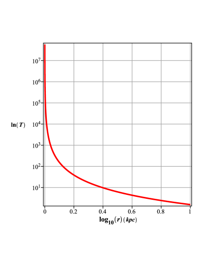
Figure 1: Non-zero scalar torsion $T$ for metric function given by (25).

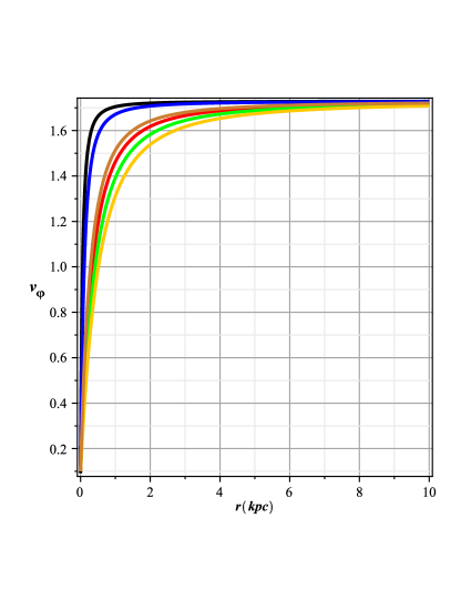
Figure 2: Toy model rotation curve for large spiral galaxy based on our $f(T)$ model. The units of the vertical axis must be read by as factor $\times 10\frac{Km}{s}$.

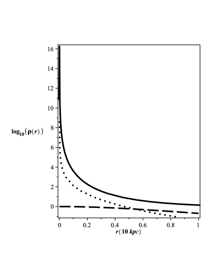
Figure 3: Two astrophysical halo density profiles in comparison to our toy model. Solid is our prediction given by (28), dot is the density of NFW model (26) and dash the estimation of pseudo-isothermal sphere approximation introduced by (27). The behavior of our model is very close to the estimations of the NFW model rho .

V On central density profile $\rho(r)$ in $f(T)$ model

From observational data we know that there exists a core with roughly constant density (mass density) in the galaxy. Many models have been proposed for this mass profile density. In brief these models are used in the numerical simulations, specially for $\Lambda$CDM:

$$\rho(r)=\frac{\rho_{i}}{(\frac{r}{r_{s}})(1+\frac{r}{r_{s}})^{2}}$$ (26)

$$\rho(r)=\frac{\rho_{0}}{1+(\frac{r}{r_{c}})^{2}}.$$ (27)

Here $\rho_{i}$ represents the density of Universe at the collapse time, $\rho_{0}$ is central density of the halo, $r_{s}$ is a characteristic radius for the halo and $r_{c}$ is the radius of the core rho . Further, very close to the center, this density profile is characterized by $r^{n}$ where $n\approx-1$, which means we have a density cusp. The observations, often favor $n\approx 0$, i.e. a constant-density core. Now we want to compare our estimation on the form of the $\rho(r)$ from model of $f(T)$ by metric function (25). Substituting (25) in (6) we obtain

$$\rho(r)=\frac{1}{16\pi}\Big{[}c_{2}+\frac{2c_{1}(1-e^{-c})}{r^{2}}\Big{]}$$ (28)

This is the exact mass profile density of our model of DM, which is comparable with the two recently proposed models of the density (26,27) (See the figure 3 for a comparison of the estimated model of us given in (28) and two models (26,27) from astrophysical data given from rho ).

VI Conclusion

In this letter we obtained the rotation curve of the galaxies in the $f(T)$ gravity. We proposed that the galaxy metric remains spherically symmetric and static. Then by solving the general equations of the metric components we obtained the lapse function $N=e^{a}$ as a function of the radial coordinate $r$. Our qualifying discussions shown a very good agreement between the rotation curves in this model and other curves obtained from the data. The scale where the velocity profile $v_{\varphi}$ attens is $v_{\varphi}\approx 10^{-3}$, which roughly corresponds to $r\approx 300$ km/s, in reasonable agreement with the data. Further, the exact mass profile density of our model of DM, is in good agreement with the two models of the density. It proves that dark matter problem can be resolved as the effect of the torsion of the space time easily.

It is well-known from ECSK theory that torsion couples to the spin of matter, hence one can infer to measure the torsion produced by any massive spinning object (including massive spiral and elliptical galaxies). However there has been assumptions about testing these theories, such as “all torsion gravity theories predict observationally negligible torsion in the solar system, since torsion (if it exists) couples only to the intrinsic spin of elementary particles, not to rotational angular momentum” tegmark . Mao et. al. have shown that Gravity Probe B is an ideal experiment for constraining several torsion based theories tegmark . Although their analysis is based on the torsion field around a uniformly rotating spherical mass such as Earth, the task of constraining torsion around massive galaxies is still open for exploration.

References

- (1) G. Bertone, Particle Dark Matter (Cambridge University Press, 2010).
- (2) G. Bertone, D. Hooper, J. Silk, Phys. Rep. 405, 279 (2005).
- (3) J. Angle, et al, Phys. Rev. Lett. 107, 051301 (2011); C. Kouvaris, P. Tinyakov, Phys. Rev. Lett. 107, 091301 (2011); A. Loeb, N. Weiner, Phys. Rev. Lett. 106, 171302 (2011); M. Jamil, D. Momeni, Chin.Phys.Lett. 28 (2011) 099801 ; H. Davoudiasl, D. E. Morrissey, K. Sigurdson, S. Tulin, Phys. Rev. Lett. 105, 211304 (2010); S. Chang, R. F. Lang, N. Weiner, Phys. Rev. Lett. 106, 011301 (2011); A. D. Simone, V. Sanz, H. P. Sato, Phys. Rev. Lett. 105, 121802 (2010); M. T. Frandsen, S. Sarkar, Phys. Rev. Lett. 105, 011301 (2010); D.Momeni, A.Azadi, Astrophys Space Sci (2008) 317: 231; T. Cohen, K. M. Zurek, Phys. Rev. Lett. 104, 101301 (2010); Y. Bai, M. Carena, J. Lykken, Phys. Rev. Lett. 103, 261803 (2009); J. McDonald, Phys. Rev. Lett. 103, 151301 (2009); P. Sikivie, Q. Yang, Phys. Rev. Lett. 103, 111301 (2009).
- (4) M. Carmeli, Int. J. Theor. Phys. 38, 1993 (1999); M. Carmeli, Int. J. Theor. Phys. 37, 2621 (1998); F. J. Oliveira, Int. J. Mod. Phys. D 15, 1963 (2006); F. J. Oliveira, arXiv:gr-qc/0508094; S. Behar, M. Carmeli, Int. J. Theor. Phys. 39, 1375 (2000); S. Behar, M. Carmeli, Int. J. Theor. Phys. 39, 1397 (2000).
- (5) T. Harko, G. Mocanu, Phys. Rev. D 85, 084012 (2012); J. Magana, T. Matos, V. Robles, A. Suarez, arXiv:1201.6107.
- (6) J. A. R. Cembranos, Phys. Rev. Lett. 102, 141301 (2009).
- (7) S. Mukohyama, Phys. Rev. D 80, 064005 (2009).
- (8) M. Carmeli, S. Malin, Int. J. Theor. Phys. 37, 2615 (1998).
- (9) L. Smalley, Phys. Lett. A 61, 436 (1977).
- (10) E. V. Linder, Phys. Rev. D 81, 127301 (2010) [Erratum-ibid. D 82, 109902 (2010)].
- (11) R. Ferraro, F. Fiorini, Phys. Rev. D 75, 084031 (2007); R. Ferraro, F. Fiorini, Phys. Rev. D 78, 124019 (2008).
- (12) M. Jamil, D. Momeni, R. Myrzakulov, Eur. Phys. J. C 72, 1959 (2012); R. Myrzakulov, Eur. Phys. J. C 71, 1752 (2011); K.K. Yerzhanov, Sh.R. Myrzakul, I.I. Kulnazarov, R. Myrzakulov, arXiv:1006.3879; K. Bamba, M. Jamil, D. Momeni, R Myrzakulov, arXiv:1202.6114; M. Jamil, D. Momeni, R. Myrzakulov, Cent. Eur. J. Phys. (2012) DOI: 10.2478/s11534-012-0103-2 P. Y. Tsyba, I. I. Kulnazarov, K. K. Yerzhanov, R. Myrzakulov, Int. J. Theor. Phys. 50, 1876 (2011); K. Bamba, R. Myrzakulov, S. Nojiri, S. D. Odintsov, Phys. Rev. D 85, 104036 (2012) ; R. Myrzakulov, arXiv:1008.4486; R. Myrzakulov,arXiv:1205.5266. P. A. Gonzalez, E. N. Saridakis, Y. Vasquez, arXiv:1110.4024.
- (13) K. Hayashi, T. Shirafuji, Phys. Rev. D 19, 3524 (1979); K. Hayashi, T. Shirafuji, Phys. Rev. D 24, 3312 (1981).
- (14) Y. D. Obukhov, J. G. Pereira, Phys. Rev. D 67, 044016 (2003); V. C. de Andrade, J. G. Pereira, Phys. Rev. D 56, 4689 (1997).
- (15) F. W. Hehl, P. v. d. Heyde, G. D. Kerlick, J. M. Nester, Rev. Mod. Phys. 48, 393 (1976).
- (16) A.V. Minkevich, Phys. Lett. B 678, 423 (2009).
- (17) M. L. Fil’chenkova, Astronomical & Astrophysical Transactions: The Journal of the Eurasian Astronomical Society 19, 115 (2000).
- (18) C. Grupen, Astroparticle Physics (Springer Verlag, 2005)
- (19) B. Nayak, M. Jamil, Phys. Lett. B 709, 118 (2012); M. Jamil, Int. J. Theor. Phys. 49, 1706 (2010); M. Jamil, A. Qadir, Gen. Relativ. Gravit. 43, 1069 (2011).
- (20) M. H. Daouda, M. E. Rodrigues, M. J. S. Houndjo, Eur. Phys. J. C 72, 1890 (2012).
- (21) B. Li, T. P. Sotiriou, J. D. Barrow, Phys. Rev. D 83, 064035 (2011).
- (22) N. Tamanini, C. G. Bohmer, arXiv:1204.4593.
- (23) D. Momeni , et al, work in progress.
- (24) J. G. Russo, A. A. Tseytlin, Nucl. Phys. B 382, 259 (1992).
- (25) F. Rahaman, M. Kalam, A. DeBenedictis, A. A. Usmani, S. Ray, Mon. Not. Roy. Astron. Soc. 389, 27 (2008).
- (26) This calculation is done most conveniently in the gauge theoretic formulation analog to visser . We will present the details in the forthcoming paper on renormalizability of the models.
- (27) M. Visser, Phys. Rev. D 80, 025011 (2009).
- (28) A. Boyarsky, A. Neronov, O. Ruchayskiy, I. Tkachev, Phys. Rev. Lett. 104, 191301 (2010); N. Fornengo, R. Lineros, M. Regis, M. Taoso, Phys. Rev. Lett. 107, 271302 (2011).
- (29) S. Capozziello, V. F. Cardone, H. Farajollahi, A. Ravanpak, Phys. Rev. D 84, 043527 (2011).
- (30) Marc S. Seigar, Y. Sofue, V. Rubin, Ann. Rev. Astron. Astrophys. 39, 137 (2001); E. Corbelli, P. Salucci, MNRAS, 311, 441 (2000); G. Angloher, et al, Eur.Phys.J. C72 , 1971(2012).
- (31) J. F. Navarro, C. S. Frenk, S. D. M. White, Ap. J. 463, 563 (1996); K. Spekkens, R. Giovanelli, M. P. Haynes, AJ, 129, 2119 (2005); W. J. G. de Blok, A. Bosma, S. McGaugh, MNRAS, 340, 657 (2003).
- (32) Y. Mao, M. Tegmark, A. Guth, S. Cabi, Phys. Rev. D 76, 104029 (2007)