Vacuum Polarization and Dynamical Chiral Symmetry Breaking: Phase Diagram of QED with Four-Fermion Contact Interaction

Abstract

We study chiral symmetry breaking for fundamental charged fermions coupled electromagnetically to photons with the inclusion of four-fermion contact self-interaction term, characterized by coupling strengths $\alpha$ and $\lambda$, respectively. We employ multiplicatively renormalizable models for the photon dressing function and the electron-photon vertex which minimally ensures mass anomalous dimension $\gamma_{m}=1$. Vacuum polarization screens the interaction strength. Consequently, the pattern of dynamical mass generation for fermions is characterized by a critical number of massless fermion flavors $N_{f}=N_{f}^{c}$ above which chiral symmetry is restored. This effect is in diametrical opposition to the existence of criticality for the minimum interaction strengths, $\alpha_{c}$ and $\lambda_{c}$, necessary to break chiral symmetry dynamically. The presence of virtual fermions dictates the nature of phase transition. Miransky scaling laws for the electromagnetic interaction strength $\alpha$ and the four-fermion coupling $\lambda$, observed for quenched QED, are replaced by a mean-field power law behavior corresponding to a second order phase transition. These results are derived analytically by employing the bifurcation analysis, and are later confirmed numerically by solving the original non-linearized gap equation. A three dimensional critical surface is drawn in the phase space of $(\alpha,\lambda,N_{f})$ to clearly depict the interplay of their relative strengths to separate the two phases. We also compute the $\beta$-functions ($\beta_{\alpha}$ and $\beta_{\lambda}$), and observe that $\alpha_{c}$ and $\lambda_{c}$ are their respective ultraviolet fixed points. The power law part of the momentum dependence, describing the mass function, implies $\gamma_{m}=1+s$, which reproduces the quenched limit trivially. We also comment on the continuum limit and the triviality of QED.

Since the works of Maskawa and Nakajima as well as the Kiev group Miransky:1976 , it is well known that quenched quantum electrodynamics (QED) exhibits vacuum rearrangement, which triggers chiral symmetry breaking when the interaction strength $\alpha=e^{2}/(4\pi)$ exceeds a critical value $\alpha_{c}\sim 1$. $\alpha_{c}$ was argued to be an ultraviolet stable fixed point defining the continuum limit in supercritical QED. Although these works were carried out for the bare vertex in the Landau gauge, principle qualitative conclusions were later shown to be robust even for the most general and sophisticated ansätze put forward henceforth for an arbitrary value of the covariant gauge parameter, see e.g., Pennington:1990 ; Gusynin:1994 ; Saul:2011 ; Bermudez:2012 . Bardeen, Leung and Love Leung:1986 demonstrated that the composite operator $\bar{\psi}\psi$ acquires large anomalous dimensions at $\alpha=\alpha_{c}$. In fact, the mass anomalous dimension was shown to be $\gamma_{m}=1$, leading to the fact that the four-fermion interaction operator $(\bar{\psi}\psi)^{2}$ acquires the scaling dimension of $d=2(3-\gamma_{m})=4$ instead of 6, and becomes renormalizable. This is an example of when an interaction which is irrelevant in a certain region of phase space (perturbative) might become relevant in another (non perturbative). Consequently, the four-fermion contact interaction becomes marginal whose absence cannot render QED a closed theory in the strong coupling domain. Depending upon the non perturbative details of the fermion-boson interaction, it is plausible to have $\gamma_{m}>1$, implying $d<4$, which would modify the status of the four-point operators from marginal to relevant, see, e.g., the review article Bashir:2005 , and references therein. The upshot of the argument is that the robustness of any conclusion about strong QED can be guaranteed only if it is supplemented by these perturbatively irrelevant operators. Quenched QED with the inclusion of these additional operators has been studied in Gorbar:1991 .

Unquenching QED involves inclusion of fermion loops. It provides screening and transforms the vacuum characteristics drastically, changing the Miransky scaling law for the dynamically generated mass $m\sim\Lambda\;{\rm Exp}[-\pi/\sqrt{\alpha/\alpha_{c}-1}]$ to a mean field square-root behavior, i.e., $m\sim\Lambda\;\sqrt{\alpha-\alpha_{c}}$, Unquenched . See also Roberts-Williams:1994 and references therein. Employing a multiplicatively renormalizable photon propagator proposed by Kizilersu and Pennington Kizilersu:2009 , it has recently been shown that large value of $N_{f}$ restores chiral symmetry above a critical value $N_{f}^{c}$ and the corresponding scaling law itself is a square-root: $m\sim\Lambda\;\sqrt{N_{f}^{c}-N_{f}}$, Calcaneo:2011 . However, these results were demonstrated without incorporating four-fermion interactions. In this article, we include this additional interaction and establish the robustness of this result with the inclusion of all the driving elements which influence chiral symmetry breaking, namely, $\alpha$: the QED interaction strength, $\lambda$: the coupling constant related to the four-fermion interactions and $N_{f}$: the fermion flavors whose effect is diametrically opposed to that of $\alpha$ and $\lambda$. We study the details of chiral symmetry breaking in the vicinity of the phase change, mapping out the phase space of all these relevant parameters and report the results which survive as well as the ones that modify in different regimes of this phase transition.

In section I, we introduce the framework of the Schwinger-Dyson equations (SDEs), the notation as well as the assumptions we employ for our analysis. Section II is dedicated to the analytic treatment of the gap equation in the neighborhood of the critical plane which separates chirally symmetric and asymmetric solutions. Next, in section III, we present the results of our numerical analysis. The last section IV summarizes our findings and provides an outlook for future work.

I SDE for the Fermion Propagator

The starting point for our analysis is the SDE for the electron propagator

$$S^{-1}(p) = S^{-1}_{0}(p)+ie^{2}\int\frac{d^{4}k}{(2\pi)^{4}}\gamma^{\mu}S(k)\Gamma^{\nu}(k,p)\Delta_{\mu\nu}(q)$$ (1)

$$- iG_{0}\,\int\frac{d^{4}k}{(2\pi)^{4}}\;{\rm Tr}[S(k)]\;,$$

where $q=k-p$, $e$ is the electromagnetic coupling and $G_{0}$ is the four-fermion coupling. We define the dimensionless four-fermion coupling $\lambda$ as $\lambda/{\Lambda^{2}}=G_{0}/(4\pi^{2})$. $S^{-1}_{0}(p)={\not\!p}$ is the inverse bare propagator for massless electrons. We parameterize the full propagator $S(p)$ in terms of the electron wave function renormalization $F(p^{2})$ and the mass function $M(p^{2})$ as $S(p)={F(p^{2})}/{({\not\!p}-M(p^{2}))}.$ $\Delta_{\mu\nu}(q)$ is the full photon propagator which can be conveniently written as

$$\Delta_{\mu\nu}(q)=-\frac{G(q^{2})}{q^{2}}\left(g_{\mu\nu}-\frac{q_{\mu}q_{\nu}}{q^{2}}\right)-\xi\frac{q_{\mu}q_{\nu}}{q^{4}}\;,$$ (2)

where $\xi$ is the covariant gauge parameter such that $\xi=0$ corresponds to the Landau gauge. $G(q^{2})$ is the photon renormalization function or the dressing function. The full electron photon vertex is represented by $\Gamma^{\mu}(k,p)$. The form of the full vertex is tightly constrained by various key properties of the gauge theory, Bashir:2005 , e.g., multiplicative renormalizability of the fermion and the gauge boson propagators, Pennington:1990 ; Bashir:1998 ; Kizilersu:2009 , perturbation theory, Bashir:2000 , the requirements of gauge invariance/covariance, Bermudez:2012 ; Ward:1950 ; Bashir-1:1994 ; Bashir-2:1996 ; Landau:1956 ; Bashir:LKF-1 and, of course, observed phenomenology, Craig:2009 . The most general decomposition of this vertex in terms of its longitudinal and transverse components is

$$\Gamma^{\mu}(k,p)=\sum_{i=1}^{4}\lambda_{i}(k,p)L_{i}^{\mu}(k,p)+\sum_{i=1}^{8}\tau_{i}(k,p)T_{i}^{\mu}(k,p)\;,$$ (3)

where $L_{1}^{\mu}=\gamma^{\mu}$, $L_{2}^{\mu}=(k+p)^{\mu}({\not\!k}+{\not\!p})$, $L_{3}^{\mu}=(k+p)^{\mu}$ and $L_{4}^{\mu}=\sigma^{\mu\nu}(k+p)_{\nu}$, where $\sigma^{\mu\nu}=[\gamma^{\mu},\gamma^{\nu}]/2$. The coefficients $\lambda_{i}$ are determined through the Ward-Takahashi identity

$$(k-p)_{\mu}\Gamma^{\mu}(k,p) = S^{-1}(k)-S^{-1}(p)\;,$$ (4)

relating the electron propagator with the electron-photon vertex, Ball:1980 . Starting from the limiting form of this identity, namely the Ward identity,

$$\frac{\partial S^{-1}(p)}{\partial p_{\mu}} = \Gamma^{\mu}(p,p)\;,$$ (5)

employing the most general form of the fermion propagator and then generalizing to arbitrarily different momenta, one obtains

$$\lambda_{1}(k,p) = \frac{1}{2}\left[\frac{1}{F(k^{2})}+\frac{1}{F(p^{2})}\right]\;,$$

$$\lambda_{2}(k,p) = \frac{1}{2}\frac{1}{k^{2}-p^{2}}\left[\frac{1}{F(k^{2})}-\frac{1}{F(p^{2})}\right]\;,$$

$$\lambda_{3}(k,p) = -\frac{1}{k^{2}-p^{2}}\left[\frac{M(k^{2})}{F(k^{2})}-\frac{M(p^{2})}{F(p^{2})}\right]\;$$ (6)

and $\lambda_{4}(k,p)=0$.

It has now been established that the choice of the transverse vertex has observable consequences at the hadronic level, despite the fact that the simple rainbow-ladder truncation is sufficient to reproduce a large body of existing experimental data on pseudoscalar and vector mesons such as their masses, charge radii, decay constants and scattering lengths, as well as their form factors and the valence quark distribution functions, Roberts-Maris:1997 ; Tandy-Maris:2000 ; Tandy-Maris:2002 ; Ji-Maris:2001 ; Tandy-Maris:1999 ; Tandy-Maris:2003 ; Maris:2002 ; Cotanch-Maris:2002 ; Bashir-Guerrero-1:2010 ; Bashir-Guerrero-2:2010 ; Tandy-Nguyen:2011 . For example, the conundrum of mass difference between opposite parity states can only be explained through corrections to the rainbow ladder truncations, Roberts-Chang:2009 , also see the review, ReviewCraig:2012 . In addition to the efforts steered through the continuum studies, attempts have also been initiated in lattice field theory to compute the transverse form factors of the fermion-boson vertex in some simple kinematical regimes, Skullerud:2003 ; Skullerud:2007 . Extending these efforts to the entire kinematical space of momenta $k^{2},p^{2}$ and $q^{2}$ is numerically challenging and it may require some time before the results are made available. However, despite the fact that the transverse vertex can have material effect on hadronic properties and is crucial in maintaining key properties of a quantum field theory, the qualitative behavior of the fermion mass function itself is not significantly sensitive to its details. Therefore, for our purpose, we shall restrict ourselves to the simplest construction (Eq. (8) of Calcaneo:2011 ) which, in the quenched limit, renders the ultraviolet behavior of $M(p^{2})$ to be

$$M(p^{2})\sim(p^{2})^{\gamma_{m}/2-1}\;,$$ (7)

with anomalous mass dimensions $\gamma_{m}=1$. This large value makes it mandatory to introduce four-point interactions to ensure self consistency. With this choice of the full vertex, we obtain, in the massless limit,

$$F(p^{2})=\left(\frac{p^{2}}{\Lambda^{2}}\right)^{\nu}\;,\quad G(q^{2})=\left(\frac{q^{2}}{\Lambda^{2}}\right)^{s}\;,$$ (8)

where $\nu=\alpha\xi/(4\pi)$ and $s=\alpha N_{f}/(3\pi)$. Near criticality, where the generated masses are small, it is reasonable to assume that the power law solutions for the propagators capture, at least qualitatively, correct description of chiral symmetry breaking. We choose to study the resulting equation for the mass function in the convenient Landau gauge. Results for any other gauge can be derived by applying the Landau-Khalatnikov-Fradkin transformations Bashir:2009 ; Bashir:LKF-1 ; Bashir:LKF-2 or using a vertex ansatz which effectively incorporates gauge covariance properties in its construction, e.g., Pennington:1990 ; Saul:2011 ; Bermudez:2012 .

After taking the trace of Eq. (1), carrying out angular integral and Wick rotating to Euclidean space, we obtain

$$M(p^{2})=g(p^{2})\int\limits_{0}^{p^{2}}dk^{2}\frac{k^{2}}{p^{2}}\frac{M(k^{2})}{k^{2}+M^{2}(k^{2})}+\int\limits_{p^{2}}^{\Lambda^{2}}dk^{2}\frac{M(k^{2})}{k^{2}+M^{2}(k^{2})}g(k^{2})+\frac{\lambda}{\Lambda^{2}}\int\limits_{0}^{\Lambda^{2}}dk^{2}\frac{k^{2}M(k^{2})}{k^{2}+M^{2}(k^{2})},$$ (9)

where $g(p^{2})=s_{0}G(p^{2})$, $s_{0}=3\alpha/(4\pi)$ and $\Lambda$ is the ultraviolet cutoff which regularizes the integrals. Note that we have employed the simplifying assumption $G(q^{2})=G(k^{2})$ for $k^{2}>p^{2}$ and $G(q^{2})=G(p^{2})$ for $p^{2}>k^{2}$, which would allow for the analytic treatment of the linearized equation for the mass function as detailed in the following section.

II Analytic Treatment

Before we venture into the computation of the mass function by numerically solving the above non-linear integral equation, we find it insightful to make analytical inroads. The differential version of the gap equation (9) simplifies in the neighborhood of the critical coupling $\alpha_{c}$; viz., the coupling whereat $M(p^{2})\neq 0$ solution bifurcates away from the $M(p^{2})=0$ solution, which alone is possible in perturbation theory. The behavior of the solution near the bifurcation point may be investigated by performing functional differentiation of the gap equation with respect to $M(p^{2})$ and evaluating the result at $M(p^{2})=0$. Practically, this amounts to analyzing linearized form of the original gap equation [i.e., the equation obtained by eliminating all terms of quadratic or higher order in $M(p^{2})$].

$$M(p^{2}) = \frac{g(p^{2})}{p^{2}}\int\limits_{0}^{p^{2}}dk^{2}M(k^{2})+\int\limits_{p^{2}}^{\Lambda^{2}}dk^{2}\frac{M(k^{2})}{k^{2}}g(k^{2})$$ (10)

$$+ \frac{\lambda}{\Lambda^{2}}\int\limits_{0}^{\Lambda^{2}}dk^{2}\;{M(k^{2})}\;.$$

Note that the non-linearized version of this equation receives negligible contribution from the region $k^{2}\rightarrow 0$, while this is not true for Eq. (10). This shortcoming is readily remedied by introducing an infrared cutoff $m^{2}$ such that $M(m)=m$. The resultant linearized gap equation, Eq. (10), can now be studied analytically in the neighborhood of the critical plane on converting it into a second order linear differential equation

$$x^{2}M^{\prime\prime}(x)+sxM^{\prime}(x)+s_{0}(1-s)\frac{M(x)}{x^{s}}=0\;,$$ (11)

with two boundary conditions. Here we have used the convenient substitution $x=\Lambda^{2}/p^{2}$. Following are the infrared and ultraviolet boundary conditions

$$M^{\prime}(\Lambda^{2}/m^{2}) = 0\;,$$ (12a)

$$M(1) = \left(1+\frac{\lambda}{s_{0}}\right)\frac{M^{\prime}(1)}{1-s}\;.$$ (12b)

Note that the four-fermion coupling only affects the ultraviolet boundary condition. The differential equation itself and the infrared boundary condition do not have any direct dependence on it. It is what we expect intuitively. four-fermion Nambu–Jona-Lasinio (NJL) type term only generates a constant mass term. Therefore, it effectively serves as a cut-off dependent bare mass and can hence only influence the dynamics through the ultraviolet boundary condition.

If we now apply the Lommel transformations: $z=Bx^{\gamma}$ and $W(x)=x^{-a}M(x)$, the linearized equation can be converted into the following Bessel differential equation

$$z^{2}W^{\prime\prime}(z)+zW^{\prime}(z)+(z^{2}-A^{2})W(z)=0\;,$$ (13)

where, $\gamma=-s/2,$ $a=(1-s)/2,$ $A=(1-s)/s,$ and $B=\sqrt{3\alpha(1-s)/(\pi s^{2})}$, where $s<1$ . The boundary conditions in terms of the function $W(z)$ are given by

$$aW(z)+\gamma zW^{\prime}(z)|_{z=B(m/\Lambda)^{s}} = 0\;,$$ (14a)

$$a\left(s_{0}-\lambda\right)W(z)-\gamma z\left(s_{0}+\lambda\right)W^{\prime}(z)|_{z=B} = 0\;.$$ (14b)

The general solution of the second order differential equation (13) is

$$W(z)=c_{1}J_{A}(z)+c_{2}Y_{A}(z)\;,$$ (15)

where $J_{A}(z)$ and $Y_{A}(z)$ are the Bessel functions of the first and the second kind, respectively. The power law part of momentum dependence of the mass function $M(x)=x^{a}W(x)$ is neatly separated out into the factor $x^{a}$, implying $\gamma_{m}=1+s$. Note that $s=1$ corresponds to a momentum independent photon propagator which implies $\gamma_{m}=2$. Consequently, Eq. (7) implies that it corresponds to a momentum independent mass function, a result which is readily and analytically confirmed from the resultant simple integral equation. This is a well known behavior of a contact interaction model of the NJL type. Moreover, the quenched limit of $\gamma_{m}=1$ is also reproduced trivially.

For the homogenous boundary conditions of Eqs. (14), the non-trivial chirally asymmetric solution of the gap equation exists if the following condition holds :

$$\left[\frac{2aJ_{A}(z)+\gamma z\left(J_{A-1}(z)-J_{A+1}(z)\right)}{2aY_{A}(z)+\gamma z\left(Y_{A-1}(z)-Y_{A+1}(z)\right)}\right]_{z=B\left(m/\Lambda\right)^{s}}=\frac{\left(1+\lambda/s_{0}\right)\gamma B\left(J_{A-1}(B)-J_{A+1}(B)\right)-(1-s)(1-\lambda/s_{0})J_{A}(B)}{\left(1+\lambda/s_{0}\right)\gamma B\left(Y_{A-1}(B)-Y_{A+1}(B)\right)-(1-s)(1-\lambda/s_{0})Y_{A}(B)}.$$ (16)

In the limit of $\Lambda\rightarrow\infty$, we obtain the following result for the dynamically generated mass $m$ :

$$\frac{m^{2}}{\Lambda^{2}}\equiv f\left(\alpha,N_{f},\lambda\right)=\left[\frac{2}{B}\right]^{\frac{2}{s}}\frac{\Gamma(A)\Gamma(A+2)2a}{\pi\gamma}\left[\frac{\left(1+\lambda/s_{0}\right)\gamma B\left(J_{A-1}(B)-J_{A+1}(B)\right)-(1-s)(1-\lambda/s_{0})J_{A}(B)}{\left(1+\lambda/s_{0}\right)\gamma B\left(Y_{A-1}(B)-Y_{A+1}(B)\right)-(1-s)(1-\lambda/s_{0})Y_{A}(B)}\right].$$ (17)

Carrying out the Taylor expansion near the critical point, we find the following scaling laws :

$$\frac{m}{\Lambda} = A_{1}\left(\alpha-\alpha_{c}\right)^{1/2}\;,\;\qquad N_{f},\lambda\;\;{\rm fixed}$$ (18)

$$\frac{m}{\Lambda} = A_{2}\left(\lambda-\lambda_{c}\right)^{1/2}\;,\;\qquad N_{f},\alpha\;\;{\rm fixed}$$ (19)

$$\frac{m}{\Lambda} = A_{3}\left(N_{f}^{c}-N_{f}\right)^{1/2}\,.\,\quad\lambda,\alpha\;\;{\rm fixed}$$ (20)

The momentum dependence of the mass function (based upon the numerical calculation discussed in the next section) and the scaling laws for $\lambda,\alpha$ and $N_{f}$ have been plotted in Figs. (1-5).

The critical values of the parameters $\alpha$, $N_{f}$, and $\lambda$ define a surface in the 3D phase-space of these parameters. The mass function is zero (non-zero) below (above) the critical surface, which corresponds to restored (broken) chiral symmetry. The analytic expression for the critical surface can be obtained by setting $m/\Lambda=0$ in equation (17). The resultant equation, which can be solved for $\lambda$, is given by

$$\lambda=-s_{0}\frac{\left[\gamma B\left(J_{A-1}(B)-J_{A+1}(B)\right)-(1-s)J_{A}(B)\right]}{\left[\gamma B\left(J_{A-1}(B)-J_{A+1}(B)\right)+(1-s)J_{A}(B)\right]}.$$ (21)

In order to obtain a finite mass for the charged fermion in the limit of $\Lambda\rightarrow\infty$, one requires charge renormalization. Therefore, in this limit, we impose $\alpha(\Lambda)=\alpha_{c}+{m^{2}}/{(A^{2}\Lambda^{2})}$. One can thus readily obtain the corresponding $\beta$-function :

$$\beta_{\alpha} = \Lambda\;\frac{\partial\alpha}{\partial\Lambda}\Big{|}_{\lambda,N_{f}}=-2(\alpha-\alpha_{c})\;.$$ (22)

Therefore, $\alpha_{c}$ is the ultraviolet fixed point of $\beta_{\alpha}$, as has been observed in Unquenched . Identical presence of the fixed point for $\beta_{\lambda}$ for $\lambda_{c}$ is readily observed :

$$\beta_{\lambda} = \Lambda\;\frac{\partial\lambda}{\partial\Lambda}\Big{|}_{\alpha,N_{f}}=-2(\lambda-\lambda_{c})\;.$$ (23)

The analytical results of this section can be confirmed and made precise through a numerical study of the non-linearized gap equation (9). This analysis is presented in the next section.

III Numerical Results

In order to compare and confirm the above analytical results, based on the linearized approximation, we solve the original non-linear integral equation (9) numerically for varying $N_{f}$, $\alpha$, and $\lambda$. Depicted in Fig. 1 is the fermion mass functions for different values of $\lambda$ for $\alpha=2.5$ and  $N_{f}=2$. The closer we get to the critical value $\lambda_{c}$, the more drastically pronounced is the drop in the mass function, indicating the approaching onslaught of the phase transition. The scaling law is explored in Fig. 2, where the variation of $m/\Lambda\equiv M(p^{2}=0)/\Lambda$ with $\lambda$ is plotted at the fixed values of $\alpha$ and $N_{f}$. The fit of the complete numerical data shows that the power of the scaling law is slightly different from 0.5. This is expected as the mean field scaling behavior (20) captures the correct physics in the immediate vicinity of the critical point, only where the linearized version of the equation becomes exact. In the same figure, we also superimpose the analytically derived square-root scaling law which, as expected, sits exactly atop the numerical findings in the immediate vicinity of the critical point. In Figs. 3 and 4, we show the variation of the mass section and the corresponding scaling law as a function of $\alpha$ at fixed values of $N_{f}=2$ and $\lambda=0.6$. These results again confirm the validity of the square-root dependence of the dynamically generated mass on the electromagnetic coupling. In Figs. 5 and 6, we plot the mass function in the presence of increasing types of virtual fermion–anti-fermion pairs and the resulting scaling law as a function of $N_{f}$, respectively, for $\alpha=2.5$ and $\lambda=0.3$. These results establish the robustness of the conclusions presented in the reference Calcaneo:2011 on the inclusion of the four-point contact interaction term.

Figure 1: The mass functions for different values of $\lambda$ at fixed $\alpha=2.5$ and $N_{f}=2$. Its increasing sensitivity to the variation in lambda helps locate the critical strength $\lambda_{c}$. Dashed and solid curves represent mass functions with (vacuum polarization of Eq. (25)) and without feedback (vacuum polarization of Eq. (8)) from the gap equation, respectively.

Figure 2: The scaling law for four-fermion coupling $\lambda$. Dots, solid and dashed lines represent numerical results, fit to the numerical data with a power law and analytically predicted square-root scaling law, respectively, at $\alpha=2.5$ and $N_{f}=2$. The mean field behavior of the chiral phase transition is evident. Dashed and solid curves represent mass functions with (vacuum polarization of Eq. (25)) and without feedback (vacuum polarization of Eq. (8)) from the gap equation, respectively.

Figure 3: The mass function $M(p^{2})$ for varying values of the electromagnetic coupling $\alpha$ for fixed values of massless fermion flavors $N_{f}=2$ and the four-fermion coupling $\lambda=0.6$. The objective is to hunt $\alpha_{c}$ and determine the nature of the phase transition. Dashed and solid curves represent mass functions with (vacuum polarization of Eq. (25)) and without feedback (vacuum polarization of Eq. (8)) from the gap equation, respectively.

Figure 4: The scaling law for the coupling $\alpha$, investigated through the behavior of the mass function near criticality, Fig. 3. Dots, solid and dashed lines represent numerical results, fit of the numerical data to the power law and analytically predicted square-root scaling law, respectively at $N_{f}=2$ and $\lambda=0.6$. Dashed and solid curves represent mass functions with (vacuum polarization of Eq. (25)) and without feedback (vacuum polarization of Eq. (8)) from the gap equation, respectively.

Figure 5: The mass function $M(p^{2})$ for increasing number of massless fermion flavors diminishes because the interaction gets screened. Chiral symmetry is restored above a certain $N_{f}^{c}$, which depends upon the values of $\alpha$ and $\lambda$. Dashed and solid curves represent mass functions with (vacuum polarization of Eq. (25)) and without feedback (vacuum polarization of Eq. (8)) from the gap equation, respectively.

Figure 6: The scaling law for $N_{f}$. Dots, solid and dashed lines represent numerical results, fit of the numerical data to the power law and analytically predicted square-root scaling law, respectively, at $\alpha=2.5$ and $\lambda=0.3$. Thus the nature of this transition is independent of the inclusion of four-fermion interaction term. Dashed and solid curves represent mass functions with (vacuum polarization of Eq. (25)) and without feedback (vacuum polarization of Eq. (8)) from the gap equation, respectively.

Figure 7: Critical curve in $\lambda-\alpha$ plane at $N_{f}=2$. Dots and solid curve represent the numerical results and analytical findings, respectively. For a fixed $N_{f}$, chiral symmetry breaking phase is achieved when the combined strength of $\alpha$ and $\lambda$ lies above the criticality curve, dictated by Eq. (21). The curve is indistinguishable, independently of the photon propagator employed [i.e., Eq. (8) or Eq. (25)]. The same is true for Figs. 8, 9 and 10.

Figure 8: Critical curve in $\lambda-N_{f}$ plane at $\alpha=2$. Dots and solid curve represent the numerical results and analytical findings, respectively. It is clear that the bifurcation analysis provides an exact analysis of the non-linear equation at criticality.

Shown in Fig. 7 is the critical curve in $\lambda-\alpha$ plane at $N_{f}=2$. The dynamical mass ceases to exist for the values of $\lambda$ and $\alpha$ below the curve. The dots in this figure represent the points obtained by numerically solving the non-linear integral equation of the mass function and the solid curve represents the analytical result which corresponds to expression (21). This criticality should be considered as an extension of its quenched QED counterpart obtained in Yamawaki:1989 . For the sake of completeness, in Figs. 8 and 9, we present the critical curves in $\lambda-N_{f}$ and $\alpha-N_{f}$ planes for fixed values of $\alpha=2$ and $\lambda=0.3$, respectively. These figures show that the analytical results agree with the numerical findings with a very good accuracy. Fig. (9) gives a quantitative picture of how the growing number of fermion flavors requires stronger electromagnetic coupling. The relation is not linear. The screening effect exhausts the strength of the interaction faster with increasing $N_{f}$.

Finally, in Fig. 10, we present the full critical surface in the phase space of $N_{f}$, $\alpha$, and $\lambda$. In the limit of $N_{f}\rightarrow 0$, Miransky scaling law is reproduced. The results presented in this paper are qualitatively robust if, instead of the multiplicatively renormalizable photon propagator of Eq. (8), we employ any of the following models :

• One loop perturbative photon propagator, as employed in Unquenched  :

  $$G(q^{2}) = 1+\frac{\alpha N_{f}}{3\pi}\;{\rm ln}\left(\frac{q^{2}}{\Lambda^{2}}\right)\;.$$ (24)

• A photon propagator which receives feedback from the gap equation, i.e.,

  $$G(q^{2}) = [\left(q^{2}+M^{2}(0)\right)/\Lambda^{2}]^{s}\;,$$ (25)

  which is also multiplicatively renormalizable. For a comparison, we have also displayed numerical results for this latter choice in all the relevant figures. As we had anticipated, near criticality, results are practically indistinguishable from the ones obtained from using the model of Eq. (8).

Note that away from criticality, a complete self consistent coupled solution of the photon and the fermion propagator will be required. However, finiteness of the dynamically generated mass for $\Lambda\rightarrow\infty$ forces non perturbative QED to be consistently defined only for those values of $\alpha$ and $\lambda$ which lie on the critical surface. This is a simple corollary of the argument laid out in Leung:1986 . Note that as we employ a model for the vacuum polarization, the running coupling is not our prediction. Following Rakow, Rakow:1991 , if we define the renormalization at $q^{2}=0$ rather than on the mass shell, we get

$$\alpha_{R}(0)=\alpha\,F_{R}^{2}(0)\,G_{R}(0)=\alpha\,G_{R}(0)\;,$$ (26)

because $F_{R}(0)=1$ for us. Therefore, our model conforms to $\alpha_{R}(0)\rightarrow 0$ in accordance with the lattice computation of unquenched QED, Rakow:1991 . As we have argued before, when $\Lambda\rightarrow\infty$, $\alpha\rightarrow\alpha_{c}$. Thus $\alpha_{R}(0)=\alpha_{c}G_{R}(0)\rightarrow 0$, which is associated with the triviality of QED in Rakow:1991 . We use this same model for the vacuum polarization even in the presence of the perturbatively irrelevant four-fermion interaction terms. This means that on the phase boundary, the renormalised coupling is zero even in the presence of the four-fermion interactions. This is in accordance with the argument presented in Roberts-Williams:1994 . However, note that for the practical solution of the gap equation, the photon propagator or the running coupling below $q^{2}=\kappa^{2}=M^{2}(\kappa^{2})$ has no bearing on chiral symmetry breaking solution.

Figure 9: Critical curve in $N_{f}-\alpha$ plane at $\lambda=0.3$. As in the other curves, dots are numerical solutions whereas the solid line is the outcome of the bifurcation analysis.

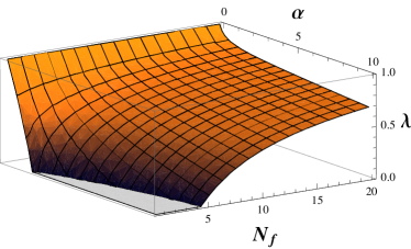
Figure 10: A three dimensional view of the criticality surface. It corresponds to Eq. (21) as well as the numerical analysis of the non-linearized Eq. (9). The region below the surface represents chirally symmetric phase.

We now recall that the Bethe-Salpeter equation gives us an approximate relation between the integral over the mass function and the "decay constant of the pion ($f$)" given by Eq. (4.42) of Roberts-Williams:1994

$$f^{2}=\int^{\Lambda}dp^{2}p^{2}M(p^{2})\;\frac{\left[M(p^{2})-p^{2}M^{\prime}(p^{2})/2\right]}{[p^{2}+M^{2}(p^{2})]^{2}}\;.$$ (27)

We numerically evaluate $f$ for varying values of $s$ and find that $f\rightarrow\infty$ in the limit when the ultraviolet regulator $\Lambda\rightarrow\infty$, a result which suggests that the continuum limit is the one of noninteracting bosons, in agreement with earlier findings Unquenched ; Kondo:1990 .

IV Epilogue

We have studied chiral symmetry breaking for fundamental fermions interacting electromagnetically with photons and self interacting through perturbatively irrelevant four-fermion contact interaction which is required to render QED a closed theory in its strongly coupled regime, where, this additional interaction becomes marginal and, perhaps, even relevant. We have used multiplicatively renormalizable models for the photon propagator (with and without the feedback from the gap equation) which, we argue, should capture the qualitative physics correctly in the vicinity of the critical surface in the phase space of $(\alpha,\lambda,N_{f})$, marking the onslaught of chiral symmetry breaking (restoration). The presence of virtual fermion–anti-fermion pairs changes the nature of the phase transitions along the $\alpha$ and $\lambda$-axes. The Miransky scaling law softens down to a square root mean field scaling behavior as a function of all the three parameters $\alpha$, $\lambda$ and $N_{f}$, (20). Study of the mass anomalous dimensions for QED with a model vacuum polarization reveals how, quantitatively, the momentum dependence of the photon propagator, i.e., $(p^{2})^{s-1}$, filters into the momentum dependence of the fermion mass function, namely, $(p^{2})^{(s-1)/2}$, through the gap equation. We believe that our analysis can and should be extended to the study of QCD through its SDEs. Situation is ripe for the application of this line of approach and technology to QCD, where we are finally having the first glimpses of the flavor dependence of the gluon propagator in the infrared region, gluon . This is for future.

Acknowledgments AB acknowledges CIC (UMICH) and CONACyT Grant Nos. 4.10, 46614-I, 128534, 94527 (Estancia de Consolidación) and the US Department of Energy, Office of Nuclear Physics, Contract No. DE-AC02-06CH11357. We thank V. Gusynin, A. Kızılers$\ddot{\rm u}$ and C.D. Roberts for useful discussions.

References

- (1) T. Maskawa and H. Nakajima, Prog. Theor. Phys. 52, 1326 (1974); P.I. Fomin and V.A. Miransky, Phys. Lett. B 64, 166 (1976); P.I. Fomin, V.P. Gusynin and V.A. Miransky, Phys. Lett. B 78, 136 (1978).
- (2) D.C. Curtis and M.R. Pennington, Phys. Rev. D 42, 4165 (1990);
- (3) D. Atkinson, J.C.R. Bloch, V.P. Gusynin, M.R. Pennington and M. Reenders, Phys. Lett. B 329, 117 (1994).
- (4) A. Bashir, A. Raya, S. Sánchez-Madrigal, Phys. Rev. D 84, 036013 (2011).
- (5) A. Bashir, R. Bermudez, L. Chang, C.D. Roberts, Phys. Rev. C 85, 045205 (2012).
- (6) W.A. Bardeen, C.N. Leung and S.T. Love, Phys. Rev. Lett. 56, 1230 (1986); C.N. Leung, S.T. Love and W.A. Bardeen, Nucl. Phys. B 273, 649 (1986).
- (7) A. Bashir and A. Raya, Trends in Boson Research, edited by A.V. Ling, Nova Science Publishers, Inc. N. Y., ISBN: 1-59454-521-9 (2005)
- (8) E.V. Gorbar, E.Sausedo, Ukr. Phys. J. 36, 1025 (1991); Manuel Reenders (Groningen U.), Ph.D. Thesis, "Dynamical symmetry breaking in the gauged Nambu-Jona-Lasinio model." e-Print: hep-th/9906034 [hep-th] (1999).
- (9) M.Salmhofer and E.Seiler, Commun. Math. Phys. 139, 395 (1991).
- (10) K. Kondo, Y. Kikukawa and H. Mino, Phys. Lett. B 220, 270 (1989); V.P. Gusynin, Mod. Phys. Lett. A 5, 133 (1990).
- (11) C.D. Roberts and A.G. Williams, Prog. Part. Nucl. Phys. 33, 477 (1994).
- (12) A. Kizilersu and M.R. Pennington, Phys. Rev. D 79, 125020 (2009).
- (13) A. Bashir, C. Calcaneo-Roldan, L.X. Gutiérrez-Guerrero and M.E. Tejeda-Yeomans, Phys. Rev. D 83, 033003 (2011).
- (14) Z. Dong, H.J. Munczek and C.D. Roberts, Phys. Lett. B 33, 536 (1994); A. Bashir, A. Kizilersu and M.R. Pennington, Phys. Rev. D 57 1242 (1998);
- (15) A. Kizilersu, M. Reenders and M.R. Pennington, Phys. Rev. D 52, 1242 (1995); A. Bashir, A. Kizilersu and M.R. Pennington, Phys. Rev. D 62, 085002 (2000); e-Print: hep-ph/9907418 [hep-th] (1999); A. Bashir and A. Raya, Phys. Rev. D 64, 105001 (2001).
- (16) J.C. Ward, Phys. Rev. 78, 1 (1950); H.S. Green, Proc. Phys. Soc. (London) A 66, 873 (1953; Y. Takahashi, Nuovo Cimento 6, 371 (1957).
- (17) A. Bashir and M.R. Pennington, Phys. Rev. D 50, 7679 (1994).
- (18) A. Bashir and M.R. Pennington, Phys. Rev. D 53, 4694 (1996).
- (19) L.D. Landau and I.M. Khalatnikov, Zh. Eksp. Teor. Fiz. 29, 89 (1956); Sov. Phys. JETP 2, 69 (1956); E.S. Fradkin, Sov. Phys. JETP 2, 361 (1956); K.Johnson and B. Zumino, Phys. Rev. Lett. 3 351 (1959).
- (20) A. Bashir, Phys. Lett. B 491, 280 (2000); A. Bashir and A. Raya, Phys. Rev. D 66 105005 (2002).
- (21) L. Chang and C.D. Roberts, Phys. Rev. Lett. 103 081601 (2009).
- (22) J.S. Ball and T-W. Chiu, Phys. Rev. D 22 2542 (1980).
- (23) P. Maris and C.D. Roberts, Phys. Rev. C 56, 3369 (1997).
- (24) P. Maris and P.C. Tandy, Phys. Rev. C 62, 055204 (2000).
- (25) P. Maris and P.C. Tandy, Phys. Rev. C 65, 045211 (2002).
- (26) C-R. Ji and P. Maris, Phys. Rev. D 64, 014032 (2001).
- (27) P. Maris and P.C. Tandy, Phys. Rev. C 60, 055214 (1999).
- (28) D. Jarecke, P. Maris and P.C. Tandy Phys. Rev. C 67, 035202 (2003).
- (29) P. Maris, PiN Newslett. 16, 213 (2002).
- (30) S.R. Cotanch and P. Maris, Phys. Rev. D 66 116010 (2002).
- (31) L.X. Gutiérrez-Guerrero, A. Bashir, I.C. Clöet and C.D. Roberts, Phys. Rev. C 81, 065202 (2010).
- (32) H.L.L. Roberts, C.D. Roberts, A. Bashir, L.X. Gutiérrez-Guerrero, P.C. Tandy, Phys. Rev. C 82, 065202 (2010).
- (33) T. Nguyen, A. Bashir, C.D. Roberts, P.C. Tandy, Phys. Rev. C 83, 062201 (2011).
- (34) L. Chang and C.D. Roberts, Phys. Rev. Lett. 103, 081601 (2009).
- (35) "Collective perspective on advances in Dyson-Schwinger Equation QCD", A. Bashir, L. Chang, I.C. Cloet, B. El-Bennich, Y-X. Liu, C.D. Roberts and P.C. Tandy, Commun. Theor. Phys. 58, 79 (2012).
- (36) J-I. Skullerud, P.O. Bowman, A. Kizilersu, D.B. Leinweber and A.G. Williams JHEP 04, 047 (2003).
- (37) A. Kizilersu, D.B. Leinweber, J-I. Skullerud and A.G. Williams, Eur. Phys. J. C 50, 871 (2007).
- (38) A. Bashir and R. Delbourgo, J. of. Phys. A 37, 6587 (2004); A. Bashir and A. Raya, Nucl. Phys. B 709, 307 (2005); Few Body Syst. 41, 185 (2007); A. Bashir and A. Raya, AIP Conf. Proc. 1026, 115 (2008); A. Bashir and A. Raya, J. Phys. Conf. Ser. 37, 90 (2006).
- (39) A. Bashir, A. Raya, S. Sánchez-Madrigal and C.D. Roberts, Few Body Sys. 46, 229 (2009).
- (40) P. O. Bowman et al., Phys. Rev. D 76, 094505 (2007); "Unquenching the gluon propagator with Schwinger-Dyson equations", A.C. Aguilar, D. Binosi, J. Papavassiliou, arXiv:1204.3868 [hep-ph], (2012); "Quark flavour effects on gluon and ghost propagators", A. Ayala, A. Bashir, D. Binosi, J. Rodríguez-Quintero, e-Print: arXiv:1208.0795 [hep-ph] (2012).
- (41) K.-I. Kondo, H. Mino and K. Yamawaki, Phys. Rev. D 39, 2430 (1990); W.A. Bardeen, S.T. Love and V.A. Miransky, Phys. Rev. D 42 3514 (1990).
- (42) P.E.L. Rakow, Nucl. Phys. B 356, 27 (1991).
- (43) K.-I. Kondo, Int. J. Mod. Phys. A 6, 5447 (1990).