Absence of finite-temperature ballistic charge transport in the 1D half-filled Hubbard model

Abstract

Finite-temperature $T>0$ transport properties of integrable and nonintegrable one-dimensional (1D) many-particle quantum systems are rather different, showing in the metallic phases ballistic and diffusive behavior, respectively. The repulsive 1D Hubbard model is an integrable system of wide physical interest. For electronic densities $n\neq 1$ it is an ideal conductor, with ballistic charge transport for $T\geq 0$. In spite that it is solvable by the Bethe ansatz, at $n=1$ its $T>0$ transport properties are a collective-behavior issue that remains poorly understood. Here we combine that solution with symmetry to show that for on-site repulsion $U>0$ the charge stiffness $D(T)$ vanishes for $T>0$ in the thermodynamic limit. This absence of finite-temperature ballistic charge transport is an exact result that clarifies a long-standing open problem.

1 Introduction

The nature of the exotic transport properties of one-dimensional (1D) correlated electronic systems at finite temperature has been a problem of long-standing interest [1, 2, 3, 4, 5, 6, 7, 8, 9]. The real part of the charge conductivity as a function of the frequency $\omega$ and temperature $T$ has the form,

$$\sigma(\omega,T)=2\pi\,D(T)\,\delta(\omega)+\sigma_{reg}(\omega,T)\,.$$ (1)

Here the charge stiffness $D(T)$ characterizes the response to a static field and $\sigma_{reg}(\omega,T)$ describes the absorption of light of frequency $\omega$. At $T>0$ the system can behave as an ideal conductor with $D(T)>0$, a normal resistor with $D(T)=0$ and $\sigma_{0}=\lim_{\omega\rightarrow 0}\sigma_{reg}(\omega,T)>0$, and an ideal insulator with $D(T)=\sigma_{0}=0$ [1, 2, 5, 6]. 1D normal conductors are typically correlated metallic nonintegrable electronic models, which show diffusive behavior such that the $T=0$ delta-fuction peak in the real part of the electrical conductivity broadens at $T>0$ into a Lorentzian Drude peak. An example of such nonintegrable systems is the 1D Hubbard-Peierls model [10]. On the other hand, 1D ideal conductors are generally correlated metallic integrable electronic systems whose real part of the electrical conductivity shows a delta-fuction peak for $T\geq 0$. That $D(T)>0$ for the latter systems, implies finite-temperature ballistic charge transport, the occurrence of an infinite set of conserving and commuting operators $\hat{Q}_{j}$ associated with the integrability preventing diffusive behavior for $T>0$ [3].

The 1D Hubbard model is solvable using the Bethe ansatz (BA) [11, 12, 13]. This technique has been useful in the calculation of static properties [14, 15, 16]. However, it has been difficult to apply to the study of transport at finite temperature. The solvable 1D Hubbard model has $D(T)>0$ for electronic densities $n=N/N_{a}\neq 1$ and temperatures $T\geq 0$ [5, 6]. This result is consistent with an exact inequality involving the integrability conservation laws, $D(T)>B(T)=1/(2k_{B}TN_{a})\sum_{j}\langle\hat{J}\hat{Q}_{j}\rangle^{2}/\langle\hat{Q}_{j}^{2}\rangle$. Here $\langle...\rangle$ stands for thermal averaging, $\hat{J}$ is the charge current operator, and $B(T)>0$ for $n\neq 1$ provides a bound for the $D(T)$ value [3, 17, 18]. However, one finds that $B(T)=0$ at $n=1$, so that the inequality is inconclusive at half filling [3]. Indeed, the charge transport at $T>0$ is not well understood for $N=N_{a}$ electrons and lattice sites. For instance, whether in the thermodynamic limit and for on-site repulsion $U>0$ the charge stiffness $D(T)$ vanishes or is finite for $T>0$ and $n=1$ remains an open issue [2, 4, 5, 6, 8, 9].

The authors of Ref. [2] have conjectured that $D(T)=0$ at $n=1$ for $U/t>0$ and $N_{a}\rightarrow\infty$. Their analysis is based both on numerical results for related integrable systems and on $D(0)=0$ exactly vanishing at $T=0$. The studies of Ref. [5] rely on the BA solution and reach the exact result that $D(T)=0$ at $n=1$ to leading order in $t^{2}/U$ for $U/t\gg 1$ and $N_{a}\rightarrow\infty$. Here $t$ is the nearest-neighbor transfer integral. On the other hand, the investigations of Ref. [4] also use the BA solution, yet predict instead that $D(T)>0$ at $n=1$ for $T>0$, $N_{a}\rightarrow\infty$, and $U/t>0$. However and as discussed below in Sec. 4, their analysis has a fatal problem at $n=1$.

In this paper we fully clarify the above mentioned unsolved long-standing problem by showing that in the thermodynamic limit, $D(T)=0$ for $T>0$ at $n=1$ and $U/t>0$. Our result definitively establishes that for $U/t>0$ the half-filled 1D Hubbard model has no ballistic charge transport and thus is not an ideal conductor. Whether for $U/t>0$ and $T>0$ it is an ideal insulator or a normal resistor remains though an interesting open issue.

2 The model global symmetry and energy eigenstates

The 1D Hubbard model reads,

$$\hat{H}=-t\sum_{\sigma}\sum_{j=1}^{N_{a}}\left[c_{j,\sigma}^{{\dagger}}\,c_{j+1,\sigma}+{\rm h.c.}\right]+U\sum_{j=1}^{N_{a}}\hat{\rho}_{j,\uparrow}\hat{\rho}_{j,\downarrow}\,.$$ (2)

Here $c_{j,\sigma}^{{\dagger}}$ creates an electron of spin projection $\sigma$ at site $j$, $\hat{\rho}_{j,\sigma}=(\hat{n}_{j,\sigma}-1/2)$, and $\hat{n}_{j,\sigma}=c_{j,\sigma}^{{\dagger}}\,c_{j,\sigma}$. The states $\eta$-spin (and spin) and $\eta$-spin projection (and spin projection) are denoted by $S_{\eta}$ and $S_{\eta}^{z}$ (and $S_{s}$ and $S_{s}^{z}$), respectively. The $S_{\alpha}$ and $S_{\alpha}^{z}$ values of the lowest-weight states (LWSs) and highest-weight states (HWSs) of the $\eta$-spin and spin algebras are such that $S_{\alpha}=-S_{\alpha}^{z}$ and $S_{\alpha}=S_{\alpha}^{z}$, respectively. Here $\alpha=\eta$ for $\eta$-spin and $\alpha=s$ for spin.

At $U=0$ the Hamiltonian of Eq. (2) becomes that of a tight-binding model, whose energy eigenstates are as well eigenstates of the current operator. One then trivially finds for $n=1$ and $N_{a}\rightarrow\infty$ that $\sigma_{reg}(\omega,T)=0$, $D(T)>0$, and max $D(T)=D(0)$, with $[D(0)-D(T)]\propto T^{2}>0$ and $D(T)\propto 1/T$ for low and high $T$, respectively. On the other hand, we find below that $D(T)=0$ for $U/t>0$. The $T\geq 0$ transition occurring at $U=U_{c}=0$ is controlled by the interplay of correlation effects with the emergence for $U/t>0$ of a hidden $U(1)$ symmetry beyond $SO(4)$ [19]. Indeed recently it was found that for $U/t\neq 0$ the global symmetry of the Hubbard model on a bipartite lattice and thus in 1D is $[SO(4)\otimes U(1)]/Z_{2}$ [19]. The eigenvalue of the generator $2\tilde{S}_{c}^{h}$ of the hidden $U(1)$ symmetry beyond $SO(4)$ is the number $2S_{c}^{h}$ of rotated-electron doubly plus unoccupied sites [19]. It is given by $2S_{c}^{h}=2[S_{\eta}+M^{\prime}]$ where $M^{\prime}$ is the number of $\eta$-spin-neutral pairs of rotated-electron doubly and unoccupied sites [19], which in 1D equals the BA number $M^{\prime}$ of Ref. [12]. The generator $2\tilde{S}_{c}^{h}$ does not commute with the charge current operator.

Importantly, the commutator $[\hat{H},2\tilde{S}_{c}^{h}]$ where $\hat{H}$ is the model Hamiltonian, Eq. (2), is finite and vanishes at $U/t=0$ and for $U/t>0$, respectively. Consistent, at $U/t=0$ the model global symmetry lacks the $U/t>0$ hidden $U(1)$ symmetry and is instead $SO(4)\otimes Z_{2}$ [19]. Here the factor $Z_{2}$ refers to a discretely generated symmetry that is an exact symmetry of the $U/t=0$ Hamiltonian but changes the sign of the interaction Hamiltonian term in $U$ when $U>0$. Taking the $U/t\rightarrow 0$ limit of the $U/t>0$ energy eigenstates leads to eigenstates of $2\tilde{S}_{c}^{h}$ that are different from the $U/t=0$ energy eigenstates, so that the problem is nonperturbative. The $U/t$ dependence of the commutator of the model Hamiltonian with the hidden $U(1)$ symmetry generator then controls the corresponding phase transition occurring at $U=U_{c}=0$ for $T\geq 0$. At $T=0$ it is the well known Mott-Hubbard metal-insulator quantum phase transition [11].

In the following we show that for $U/t>0$ the $D(T)$ value is determined by collective behavior stemming from the interplay of the correlation effects with the algebra associated with the commutators of the $\eta$-spin $SU(2)$ symmetry generators with several charge current operators. For $U/t>0$ the model’s BA solution has two alternative representations that refer to subspaces spanned either by the LWSs or HWSs of both $SU(2)$ symmetry algebras, respectively. In this paper we consider the LWS BA representation for which the numbers,

$$n_{\eta} = S_{\eta}+S_{\eta}^{z}=0,1,...,2S_{\eta}\,,$$

$$n_{s} = S_{s}+S_{s}^{z}=0,1,...,2S_{s}\,,$$ (3)

vanish, where $S_{\eta}^{z}=-(N_{a}-N)/2$ and $S_{s}^{z}=-(N_{\uparrow}-N_{\downarrow})/2$. We call Bethe states the energy eigenstates contained in the BA subspace, which are LWSs of both the $\eta$-spin and spin algebras. The spin non-LWSs are generated from such Bethe states by a transformation similar to that reported in the following for the $\eta$-spin non-LWSs, which involves the spin off-diagonal generators. However, concerning the spin degrees of freedom our analysis considers general states, which may be spin LWSs or spin non-LWSs. Indeed the spin algebra plays no active role in our study.

For $U/t>0$ the $4^{N_{a}}$ energy eigenstates $|l_{\rm r},S_{\eta},S_{\eta}^{z}\rangle$ are as well eigenstates of the hidden $U(1)$ symmetry generator $2\tilde{S}_{c}^{h}$, which counts the number of rotated-electron doubly plus unoccupied sites [19]. Within our notation, $l_{\rm r}$ stands for all quantum numbers beyond $S_{\eta}$ and $S_{\eta}^{z}$ needed to uniquely define a $U/t>0$ energy eigenstate, $|l_{\rm r},S_{\eta},S_{\eta}^{z}\rangle$. The $\eta$-spin non-LWSs are generated from the corresponding $n_{\eta}=0$ $\eta$-spin LWS $|l_{\rm r},S_{\eta},-S_{\eta}\rangle$ as follows,

$$|l_{\rm r},S_{\eta},S_{\eta}^{z}\rangle=|l_{\rm r},S_{\eta},-S_{\eta}+n_{\eta}\rangle=\frac{1}{\sqrt{{\cal{C}}_{\eta}}}({\hat{S}}^{+}_{\eta})^{n_{\eta}}|l_{\rm r},S_{\eta},-S_{\eta}\rangle\,.$$ (4)

Here $n_{\eta}=1,...,2S_{\eta}$,

$${\cal{C}}_{\eta}=\langle l_{\rm r},S_{\eta},-S_{\eta}|({\hat{S}}_{\eta}^{-})^{n_{\eta}}({\hat{S}}^{+}_{\eta})^{n_{\eta}}|l_{\rm r},S_{\eta},-S_{\eta}\rangle=[n_{\eta}!]\prod_{j=1}^{n_{\eta}}[\,2S_{\eta}+1-j\,]\,,$$ (5)

is a normalization constant and the $\eta$-spin generators read,

$${\hat{S}}^{+}_{\eta} = \sum_{j=1}^{N_{a}}(-1)^{j}\,c_{j,\downarrow}^{{\dagger}}\,c_{j,\uparrow}^{{\dagger}}\,;\hskip 7.11317pt{\hat{S}}_{\eta}^{-}=({\hat{S}}_{\eta}^{+})^{{\dagger}}\,;\hskip 7.11317pt{\hat{S}}_{\eta}^{z}={1\over 2}\sum_{j=1}^{N_{a}}(\hat{\rho}_{j,\uparrow}+\hat{\rho}_{j,\downarrow})\,,$$

$$(\hat{\vec{S}}_{\eta})^{2} = (\hat{S}_{\eta}^{z})^{2}+{1\over 2}(\hat{S}_{\eta}^{+}\hat{S}_{\eta}^{-}+\hat{S}_{\eta}^{-}\hat{S}_{\eta}^{+})\,,$$ (6)

where we have also provided the diagonal generator and $(\hat{\vec{S}}_{\eta})^{2}$ expressions. Importantly, the half-filling energy eigenstates, which are those of most interest for our study, refer in Eq. (4) to $n_{\eta}=S_{\eta}$.

Except for a constant pre-factor, the charge current operator $\hat{J}^{\rho}$ equals the $z$-axis $\eta$-spin current operator $\hat{J}^{\sigma_{z}^{\eta}}$,

$$\hat{J}^{\rho} = (e)\,\hat{J}\,;\hskip 14.22636pt\hat{J}^{\sigma_{z}^{\eta}}=(1/2)\,\hat{J}\,,$$

$$\hat{J} = -i\,t\sum_{\sigma}\sum_{j=1}^{N_{a}}\left[c_{j,\sigma}^{{\dagger}}\,c_{j+1,\sigma}-c_{j+1,\sigma}^{{\dagger}}\,c_{j,\sigma}\right]\,,$$ (7)

where $e$ denotes the electronic charge.

Our main goal is to calculate the charge stiffness $D(T)$ for $U/t>0$ and $S_{\eta}^{z}=0$, which in the thermodynamic limit involves only current expectation values and can be written in terms of a sum over the $S_{\eta}^{z}=0$ half-filling states, Eq. (4), as [3, 5],

$$2\pi D(T)={\pi\over k_{B}TN_{a}}\sum_{l_{\rm r}}\sum_{S_{\eta}=0,1,2,...,N_{a}/2}p_{l,S_{\eta}}|\langle l_{\rm r},S_{\eta},0|\hat{J}|l_{\rm r},S_{\eta},0\rangle|^{2}\,.$$ (8)

Here $p_{l_{\rm r},S_{\eta}}=e^{-\epsilon_{l_{\rm r},S_{\eta}}/k_{B}T}/Z$ is the usual Boltzmann weight and the partition function reads $Z=\sum_{l_{\rm r},S_{\eta}}e^{-\epsilon_{l_{\rm r},S_{\eta}}/k_{B}T}$.

3 current matrix elements and expectation values

The following commutators play a major role in our study,

$$\left[\hat{J},\hat{S}_{\eta}^{z}\right] = 0\,;\hskip 14.22636pt\left[\hat{J},(\hat{\vec{S}}_{\eta})^{2}\right]=\hat{J}^{+}\hat{S}_{\eta}^{-}-\hat{S}_{\eta}^{+}\hat{J}^{-}$$

$$\left[\hat{J},\hat{S}_{\eta}^{\pm}\right] = \left[\hat{S}_{\eta}^{z},\hat{J}^{\pm}\right]=\pm\hat{J}^{\pm}\,;\hskip 14.22636pt\left[\hat{J}^{\pm},\hat{S}_{\eta}^{\mp}\right]=\pm 2\hat{J}\,,$$ (9)

where $\hat{J}^{\pm}$ denotes the following current operators related to the $\eta$-spin $SU(2)$ symmetry algebra,

$$\hat{J}^{+}=i\,2t\sum_{j=1}^{N_{a}}(-1)^{j}\left[c_{j,\downarrow}^{{\dagger}}\,c_{j+1,\uparrow}^{{\dagger}}+c_{j+1,\downarrow}^{{\dagger}}\,c_{j,\uparrow}^{{\dagger}}\right]\,;\hskip 14.22636pt\hat{J}^{-}=(\hat{J}^{+})^{{\dagger}}\,.$$ (10)

The $S_{\eta}>0$ metallic $\eta$-spin LWSs $|l_{\rm r},S_{\eta},-S_{\eta}\rangle$ and half-filling simultaneously $\eta$-spin LWSs and HWSs $|l_{\rm r},0,0\rangle$ used in our operator algebra manipulations obey the following well-known transformation laws,

$$\hat{S}_{\eta}^{-}|l_{\rm r},S_{\eta},-S_{\eta}\rangle = 0\,,$$

$$\hat{S}_{\eta}^{+}|l_{\rm r},0,0\rangle = \hat{S}_{\eta}^{-}|l_{\rm r},0,0\rangle=0\,,$$ (11)

which trivially follow from the $\eta$-spin $SU(2)$ symmetry algebra.

In order to evaluate the current expectation values $\langle l_{\rm r},S_{\eta},0|\hat{J}|l_{\rm r},S_{\eta},0\rangle$ that appear in the charge-stiffness expression, Eq. (8), in the following we consider a more general problem: That of finding from operator-algebra symmetry alone some of the general current matrix elements,

$$\langle l_{\rm r},S_{\eta},S_{\eta}^{z}|\hat{J}|l_{\rm r},S_{\eta}^{\prime},S_{\eta}^{z}\rangle = {1\over\sqrt{{\cal{C}}_{\eta}{\cal{C}}_{\eta}^{\prime}}}$$ (12)

$$\times \langle l_{\rm r},S_{\eta},-S_{\eta}|({\hat{S}}_{\eta}^{-})^{n_{\eta}}\hat{J}({\hat{S}}^{+}_{\eta})^{n_{\eta}^{\prime}}|l_{\rm r},S_{\eta}^{\prime},-S_{\eta}^{\prime}\rangle\,,$$

that vanish. Here $n_{\eta}=S_{\eta}+S_{\eta}^{z}$, $n_{\eta}^{\prime}=S_{\eta}^{\prime}+S_{\eta}^{z}$, the normalization constants are given in Eq. (5), and we have accounted for the vanishing of the commutator $[\hat{J},\hat{S}_{\eta}^{z}]=0$, Eq. (9), so that the current operator only connects states with the same $S_{\eta}^{z}$ value. For $l{\rm r}=l{\rm r}^{\prime}$, $S_{\eta}=S_{\eta}^{\prime}$, and $S_{\eta}^{z}=0$ Eq. (13) refers to the current expectation values in Eq. (8).

To double check our results on the current expectation values, we find their value from limiting cases of two different classes of current matrix elements: (a) matrix elements $\langle l_{\rm r},S_{\eta},0|\hat{J}|l_{\rm r},S_{\eta}^{\prime},0\rangle$ between $S_{\eta}^{z}=0$ half-filling states with arbitrary $S_{\eta}$ and $S_{\eta}^{\prime}$ values, respectively, and (b) matrix elements $\langle l_{\rm r},S_{\eta},S_{\eta}^{z}|\hat{J}|l_{\rm r},S_{\eta},S_{\eta}^{z}\rangle$ between states with the same $S_{\eta}>0$ and $S_{\eta}^{z}$ arbitrary values. While the current matrix elements of type (a) connect only half-filling states those of type (b) may connect $S_{\eta}^{z}>0$ metallic states.

By combining the systematic use of the commutators given in Eq. (9) with the transformation laws of Eq. (11), we reach the following general useful result concerning the current matrix elements of type (a),

$$\langle l_{\rm r},S_{\eta},0|\hat{J}|l_{\rm r},S_{\eta}+\delta S_{\eta},0\rangle=0\,,\hskip 14.22636pt\delta S_{\eta}\neq\pm 1\,.$$ (13)

For half-filling states whose generation from metallic $\eta$-spin LWSs involves small $n_{\eta}=(S_{\eta}-S_{\eta}^{z})$ values, the calculations are straightforward. They become lengthly as the $n_{\eta}$ value increases, yet remain straightforward.

Furthermore, by use of similar techniques we find after a suitable operator algebra involving commutator manipulations and state transformations the following relation between current matrix elements of type (b),

$$\langle l_{\rm r},S_{\eta},S_{\eta}^{z}|\hat{J}|l_{\rm r}^{\prime},S_{\eta},S_{\eta}^{z}\rangle=C(2S_{\eta},n_{\eta})\,\langle l_{\rm r},S_{\eta},-S_{\eta}|\hat{J}|l_{\rm r}^{\prime},S_{\eta},-S_{\eta}\rangle\,,$$ (14)

where $S_{\eta}^{z}=-S_{\eta}+n_{\eta}$ and $n_{\eta}=1,...,2S_{\eta}$. The coefficient $C(l,\tilde{l})$ appearing here is such that,

$$C(l,\tilde{l}) = -C(l,l-\tilde{l})\,,\hskip 9.95863pt\tilde{l}\leq l/2\,,$$

$$C(l,l/2) = 0\hskip 4.26773pt{\rm for}\hskip 4.26773ptl/2\hskip 4.26773pt{\rm integer}\,.$$ (15)

The result $C(l,l/2)=0$ follows from the first equality for $\tilde{l}=l/2$, where we have denoted $2S_{\eta}$ and $n_{\eta}$ by $l$ and $\tilde{l}$, respectively.

First, it follows from Eq. (13) for $l_{\rm r}=l_{\rm r}^{\prime}$ and $\delta S_{\eta}=0$ that the expectation values of all half-filling energy eigenstates $|l_{\rm r},S_{\eta},0\rangle$ vanish, $\langle l_{\rm r},S_{\eta},0|\hat{J}|l_{\rm r},S_{\eta},0\rangle=0$. Second, for $S_{\eta}>0$ such half-filling states have numbers $S_{\eta}=n_{\eta}=1,2,...,N_{a}/2$, so that $C(2S_{\eta},n_{\eta})=C(2S_{\eta},S_{\eta})=0$, as given in Eq. (15). Consistent with the vanishing current expectation values of all $S_{\eta}\geq 0$ found from Eq. (13), it follows from Eq. (14) that the current expectation value of $S_{\eta}>0$ half-filling states $|l_{\rm r},S_{\eta},0\rangle$ vanishes.

We have then confirmed that the analysis of the two classes of current matrix elements leads to the same result, that for $U/t>0$ the charge current expectation values $\langle l_{\rm r},S_{\eta},0|\hat{J}|l_{\rm r},S_{\eta},0\rangle$ vanish for all $n=1$ energy eigenstates. In contrast, the current expectation values $\langle l_{\rm r},S_{\eta},S_{\eta}^{z}|\hat{J}|l_{\rm r},S_{\eta},S_{\eta}^{z}\rangle$ of $S_{\eta}^{z}\neq 0$ metallic states are in general finite [20, 21].

$S_{\eta}\backslash n_{\eta}$	$0$	$1$	$2$	$3$	$4$	$5$	$6$	$7$
1/2	1	-1	-	-	-	-	-	-
1	1	0	-1	-	-	-	-	-
3/2	1	1/3	-1/3	-1	-	-	-	-
2	1	1/2	0	-1/2	-1	-	-	-
5/2	1	3/5	1/5	-1/5	-3/5	-1	-	-
3	1	2/3	1/3	0	-1/3	-2/3	-1	-
7/2	1	5/7	9/16	1/7	-1/7	-9/6	-5/7	-1

Table 1: The coefficient $C(2S_{\eta},n_{\eta})$ on the right-hand side of Eq. (14) for the $\eta$-spin-tower states of $\eta$-spin up to $S_{\eta}=7/2$. At half filling one has that $S_{\eta}=0,1,2,3$ is an integer and $S_{\eta}^{z}=0$, so that $n_{\eta}=S_{\eta}$ and $C(2S_{\eta},S_{\eta})=0$.

Only the coefficient $C(2S_{\eta},n_{\eta})=C(2S_{\eta},S_{\eta})=0$ in Eqs. (14) and (15) is needed for our $n=1$ study. A general expression of that coefficient which applies to $n_{\eta}=0,1,2,3$ and any $\eta$-spin value $S_{\eta}\leq n_{\eta}/2$ is,

$$C(l,\tilde{l}) = {1\over[\tilde{l}!]\prod_{j=1}^{\tilde{l}}[\,l+1-j\,]}[\prod_{j=1}^{\tilde{l}}[\,jl-2^{j}\,]-(\tilde{l}-1)(2[(l+1)-(\tilde{l}-1)])^{\tilde{l}-1}$$ (16)

$$- (1-\delta_{\tilde{l},1})(l\tilde{l}-2^{\tilde{l}})(\tilde{l}-2)(2[(l+1)-(\tilde{l}-2)])^{\tilde{l}-2}]\,,\hskip 9.95863pt\tilde{l}=1,2,3\,,\hskip 9.95863ptl\geq\tilde{l}\,,$$

where $l\equiv 2S_{\eta}$ and $\tilde{l}\equiv n_{\eta}$. For $n_{\eta}>3$ the $C(2S_{\eta},n_{\eta})$ expression becomes too cumbersome for $S_{\eta}\neq n_{\eta}$ metallic states and vanishes for half-filling $S_{\eta}=n_{\eta}$ states. Combining the expression of Eq. (16) with the relation $C(l,\tilde{l})=-C(l,l-\tilde{l})$ provided in Eq. (15) for $\tilde{l}\leq l/2$, we have calculated the coefficient $C(2S_{\eta},n_{\eta})$ of all states with $\eta$-spin $S_{\eta}\leq 7/2$, whose values are given in Table 1.

4 The charge stiffness and regular conductivity at half filling

Our above result that the current expectation values of all $U/t>0$ half-filling energy eigenstates $|l_{\rm r},S_{\eta},0\rangle$ vanish implies according to Eq. (8) that the charge stiffness $D(T)$ vanishes in the thermodynamic limit. Hence we have just showed that at half filling it vanishes for $U/t>0$ and $T>0$ in the thermodynamic limit, whereas $D(T)>0$ at $U/t=0$. This is our main result, which clarifies a long-standing open problem. Note however that the conductivity sum rule $\int d\omega\,\sigma(\omega,T)$ remains invariant under the transition occurring at $U=U_{c}=0$ for all temperatures. Indeed, we find that $2\pi\,D(T)|_{U/t=0}=\lim_{U/t\rightarrow 0}\int d\omega\,\sigma_{reg}(\omega,T)>0$ and $\lim_{U/t\rightarrow 0}2\pi\,D(T)=\left[\int d\omega\,\sigma_{reg}(\omega,T)\right]|_{U/t=0}=0$.

We emphasize that our exact result that $D(T)$ vanishes at $n=1$ for $U/t>0$ and $T\geq 0$ does not apply to the model on a finite 1D lattice. For it the charge stiffness expression has additional terms, beyond those given in Eq. (8), which vanish in the present thermodynamic limit [3]. Such extra terms involve current matrix elements between pairs of degenerate energy eigenstates. Moreover, our exact results disagree with the prediction of Ref. [4] that $D(T)$ should be finite in the thermodynamic limit for $U/t>0$ and $n=1$. That prediction error stems from some of the separate integrals of the individual summands occurring in the integrands of Eq. (25) of Ref. [4], which diverge at $n=1$. That turns out to be a fatal problem, similar to that of some of the integrands of Eqs. (24) and (25) of Ref. [7] for a related BA solvable model, as was discussed and recognized in that reference. On the other hand, the studies of Ref. [8] did not calculate explicitly the charge currents carried by $S_{\eta}^{z}=0$ states with $S_{\eta}>0$ and assumed those to be finite, alike for the metallic states of the same $\eta$-spin-$S_{\eta}$ tower, yet they vanish.

Our results allow two possible scenarios for the 1D half-filled Hubbard model phase at a given finite temperature $T$: Either the model behaves as a normal resistor with $D(T)=0$ and $\sigma_{0}=\lim_{\omega\rightarrow 0}\sigma_{reg}(\omega,T)>0$ or as an ideal insulator with $D(T)=\sigma_{0}=0$. The use of Eq. (13) allows the simplification of the standard linear-response theory expression of $\sigma_{reg}(\omega,T)$ to,

$$\sigma_{reg}(\omega,T)={\pi\left(1-e^{-\omega/(k_{B}\,T)}\right)\over N_{a}\,\omega}\sum_{l_{\rm r}}\sum_{S_{\eta}=0,1,2,...,N_{a}/2}p_{l_{\rm r},S_{\eta}}\sum_{j=\pm 1}\Theta(S_{\eta}+j)$$ (17)

$$\times \sum_{l_{\rm r}^{\prime},(\epsilon_{l_{\rm r}^{\prime},S_{\eta}+j}\neq\epsilon_{l_{\rm r},S_{\eta}})}|\langle l_{\rm r},S_{\eta},0|\hat{J}|l_{\rm r}^{\prime},S_{\eta}+j,0\rangle|^{2}\delta(\omega-\epsilon_{l^{\prime},S_{\eta}+j}+\epsilon_{l,S_{\eta}})\,.$$

Here $\Theta(x)=1$ for $x\geq 0$ and $\Theta(x)=0$ for $x<0$.

For $U/t>0$ the exact ground state of the half-filled Hubbard model at zero chemical potential and zero spin density, which here we denote by $|GS,0,0\rangle$, is a $\eta$-spin singlet, $S_{\eta}=0$, with $M^{\prime}=0$ [11, 12], so that it is an eigenstate of the hidden $U(1)$ symmetry generator with eigenvalue $2S_{c}^{h}=2[S_{\eta}+M^{\prime}]=0$. Moreover, the exact minimum energy for transitions from that ground state to two-electron charge and $\eta$-spin excited states with $2S_{c}^{h}=2[S_{\eta}+M^{\prime}]>0$ is min $\Delta_{D_{rot}}=2\Delta_{MH}\,[S_{\eta}+M^{\prime}]$. Here $2\Delta_{MH}$ is the Mott-Hubbard gap, which at zero spin density behaves as $\sim{8\over\pi}\sqrt{t\,U}\,e^{-2\pi\left({t\over U}\right)}$ for $U/t\ll 1$ and $\sim(U-4t)$ for $U/t\gg 1$ [11]. The minimum excitation energy, min $\epsilon_{l^{\prime},1}-\epsilon_{GS,0}=2\Delta_{MH}$, relative to the $S_{\eta}=0$ ground state whose matrix element $\langle GS,0,0|\hat{J}|l_{\rm r}^{\prime},1,0\rangle$ in Eq. (17) does not vanish refers to excited energy eigenstates $|l_{\rm r}^{\prime},1,0\rangle$ with $S_{\eta}=1$ and $2S_{c}^{h}=2$. Hence at $T=0$ we find that $\sigma_{reg}(\omega,0)=0$ for $\omega<2\Delta_{MH}$. This confirms that the real part of the conductivity vanishes for the $T=0$ Mott-Hubbard insulator for energies smaller than the Mott-Hubbard gap.

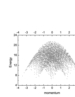
Figure 1: The degenerate energy spectrum of several types of $2S_{c}^{h}=2[S_{\eta}+M^{\prime}]=4$ states for $U/t=6$ and $N_{a}=30$. This includes the $S_{\eta}=2;M^{\prime}=0$ states, $S_{\eta}=1;M^{\prime}=1$ states, and $S_{\eta}=0;M^{\prime}=2$ states considered in the text.

To characterize possible $T>0$ transitions for which $\epsilon_{l_{\rm r}^{\prime},S_{\eta}\pm 1}-\epsilon_{l_{\rm r},S_{\eta}}\rightarrow 0$ in Eq. (17), it is convenient to replace the quantum number $l_{\rm r}$ in $|l_{\rm r},S_{\eta},S_{\eta}^{z}\rangle$ by two quantum numbers, $m_{\rm r},M^{\prime}$, so that $|m_{\rm r},M^{\prime},S_{\eta},S_{\eta}^{z}\rangle\equiv|l_{\rm r},S_{\eta},S_{\eta}^{z}\rangle$. Here $m_{\rm r}$ stands now for all quantum numbers beyond $M^{\prime}$, $S_{\eta}$, and $S_{\eta}^{z}$ needed to uniquely define the $U/t>0$ energy eigenstate. From analysis of the half-filling energy spectra obtained by combining the BA solution with symmetry, we then find that $\epsilon_{m_{\rm r}^{\prime},M^{\prime}-1,S_{\eta}}-\epsilon_{m_{\rm r},M^{\prime},S_{\eta}-1}\rightarrow 0$ for pairs of states with the same hidden $U(1)$ symmetry generator eigenvalue $2S_{c}^{h}=2[S_{\eta}+M^{\prime}]$ and suitable $m_{\rm r}$ and $m_{\rm r}^{\prime}$ values. Specifically, provided that the matrix elements of the following form are finite,

$$\langle m_{\rm r},M^{\prime},S_{\eta}-1,0|\hat{J}|m_{\rm r}^{\prime},M^{\prime}-1,S_{\eta},0\rangle|_{S_{\eta}=M^{\prime}}={1\over\sqrt{{\cal{C}}_{\eta}{\cal{C}}_{\eta}^{\prime}}}$$ (18)

$$\times \langle m_{\rm r},M^{\prime},S_{\eta}-1,-S_{\eta}+1|({\hat{S}}_{s}^{-})^{M^{\prime}-1}\hat{J}({\hat{S}}^{+}_{\eta})^{M^{\prime}}|m_{\rm r}^{\prime},M^{\prime}-1,S_{\eta},-S_{\eta}\rangle|_{S_{\eta}=M^{\prime}}$$

$$= {1\over\sqrt{C_{M^{\prime}}}}\langle m_{\rm r},M^{\prime},S_{\eta}-1,-S_{\eta}+1|\hat{J}^{+}|m_{\rm r}^{\prime},M^{\prime}-1,S_{\eta},-S_{\eta}\rangle|_{S_{\eta}=M^{\prime}}\,,$$

where $M^{\prime}=1,2,...$ and the two states are such that $\epsilon_{m_{\rm r}^{\prime},M^{\prime}-1,S_{\eta}}-\epsilon_{m_{\rm r},M^{\prime},S_{\eta}-1}\rightarrow 0$, then $\sigma_{0}=\lim_{\omega\rightarrow 0}\sigma_{reg}(\omega,T)$ would be finite for $T>0$. Note that the states $|m_{\rm r}^{\prime},M^{\prime}-1,S_{\eta},-S_{\eta}\rangle$ and $|m_{\rm r},M^{\prime},S_{\eta}-1,-S_{\eta}+1\rangle$ connected in Eq. (18) by the two-electron current operator $\hat{J}^{+}$, Eq. (10), have $N=N_{a}-2M^{\prime}$ and $N+2=N_{a}-2M^{\prime}+2$ electrons, respectively.

In case that such matrix elements were finite, their absolute value would decrease rapidly upon increasing $M^{\prime}$ and a large fraction of the weight would be generated by the $M^{\prime}=1$ transition. (The constant $C_{M^{\prime}}$ in the last expression given in Eq. (18) reads $C_{1}=2$ and $C_{2}=3$ for $M^{\prime}=1$ and $M^{\prime}=2$, respectively.) Unfortunately, we could not evaluate such matrix elements. The numerical results of Ref. [6] refer to finite systems and provide some evidence that $\sigma_{0}$ could be finite in the thermodynamic limit for $U/t>0$ and $T\rightarrow\infty$. Nonetheless an ultimate prove that for $U/t>0$ the conductivity $\sigma_{0}$ vanishes or is finite remains lacking.

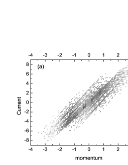
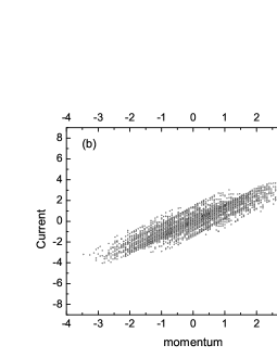
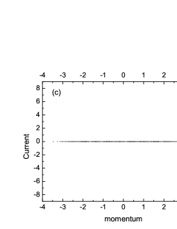
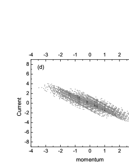
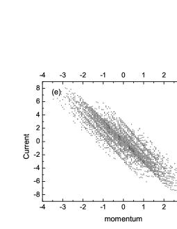
Figure 2: The current spectra of (a) the metallic $S_{\eta}=2;S_{\eta}^{z}=-2;M^{\prime}=0$ states, (b) metallic $S_{\eta}=2;S_{\eta}^{z}=-1;M^{\prime}=0$ states, (c) half-filling $S_{\eta}=2;S_{\eta}^{z}=0;M^{\prime}=0$ states, $S_{\eta}=1;S_{\eta}^{z}=0;M^{\prime}=1$ states, and $S_{\eta}=S_{\eta}^{z}=0;M^{\prime}=2$ states, (d) metallic $S_{\eta}=2;S_{\eta}^{z}=1;M^{\prime}=0$ states, and (e) metallic $S_{\eta}=2;S_{\eta}^{z}=2;M^{\prime}=0$ states considered in the text for $U/t=6$ and $N_{a}=30$.

5 Current spectra of degenerate half-filling and metallic states

In order to illustrate that $n=1$ and $n\neq 1$ energy eigenstates whose energy spectra are degenerate carry when $U/t>0$ zero and finite charge current, respectively, we have derived numerically the current expectation value and energy spectra of a set of related energy eigenstates with $2S_{c}^{h}=2[S_{\eta}+M^{\prime}]=4$ and thus four holes in the $c$ momentum band [22]. The energy spectrum of the simpler energy eigenstates with $2S_{c}^{h}=2[S_{\eta}+M^{\prime}]=2$ were studied and plotted in Ref. [21]. Such states have two holes in the $c$ momentum band [22] and include three types of $S_{\eta}^{z}=0,\pm 1$; $S_{\eta}=1$; $M^{\prime}=0$ states and the $S_{\eta}=-S_{\eta}^{z}=0$; $M^{\prime}=1$ states. Only the charge current spectrum of the metallic $S_{\eta}^{z}=-1$; $S_{\eta}=1$; $M^{\prime}=0$ states was plotted in Ref. [21]. On the other hand, the charge currents carried by the also metallic $S_{\eta}^{z}=+1$; $S_{\eta}=1$; $M^{\prime}=0$ states is minus that of the $S_{\eta}^{z}=-1$; $S_{\eta}=1$; $M^{\prime}=0$ states. Moreover, the half-filling $\eta$-spin-triplet $S_{\eta}^{z}=0$; $S_{\eta}=1$; $M^{\prime}=0$ states and half-filling $\eta$-spin-singlet $S_{\eta}=-S_{\eta}^{z}=0$; $M^{\prime}=1$ states carry no current in the thermodynamic limit.

Here we consider five types of $S_{\eta}^{z}=0,\pm 1,\pm 2$; $S_{\eta}=2$; $M^{\prime}=0$ states, three types of $S_{\eta}^{z}=0,\pm 1$; $S_{\eta}=1$; $M^{\prime}=1$ states, and two types of $S_{\eta}=-S_{\eta}^{z}=0$; $M^{\prime}=2$ states with two and one occupied BA quantum number $J^{{}^{\prime}1}_{\alpha}$ and $J^{{}^{\prime}2}_{\alpha}$ of Ref. [12], respectively. The degenerate energy spectrum of such states is plotted in Fig. 1. The current spectra of the energy eigenstates with $2S_{c}^{h}=2[S_{\eta}+M^{\prime}]=4$ and $\eta$-spin $S_{\eta}=0$ and $S_{\eta}=2$ are plotted in Fig. 2. The spectra of Figs. 1,2(a) were calculated from the BA for $U/t=6$ and $N_{a}=30$. Consistent with the results of this paper, the current of the $n=1$ states plotted in Fig. 2(c) vanishes. The metallic states whose currents are plotted in Figs. 2(a),(b),(d),(e) have the same energy as these $n=1$ states yet carry finite charge current.

6 Conclusions

Recently the finite-energy behavior of correlation functions of 1D correlated systems [23, 24, 25, 26] has been found to differ signi cantly from the linear Luttinger liquid theory predictions [14]. Here we have considered the related problem of the exotic $T>0$ charge transport properties of the half-filled 1D Hubbard model. We have shown that for $U/t>0$ its charge stiffness $D(T)$ vanishes for $T>0$ in the thermodynamic limit. The corresponding absence of finite-temperature ballistic charge transport is an exact result that clarifies a long-standing open problem.

Whether for the half-filled 1D Hubbard model $\sigma_{0}=\lim_{\omega\rightarrow 0}\sigma_{reg}(\omega,T)$ vanishes or is finite for $T>0$ and $U/t>0$ in the thermodynamic limit is an interesting related open issue that deserves further investigations.

Acknowledgments

We thank H. Johannesson, H. Q. Lin, N. M. R. Peres, and P. D. Sacramento for discussions, the hospitality and support of the Beijing Computational Science Research Center, and the support of the Research Grants Council of Hong Kong under the Project CUHK401108. J. M. P. C. thanks the hospitality of the University of Gothenburg and the support by the FEDER through the COMPETE Program, Portuguese FCT both in the framework of the Strategic Project PEST-C/FIS/UI607/2011 and under SFRH/BSAB/1177/2011, and the Swedish Foundation for International Cooperation in Research and Higher Education (Grant. No. IG2011-2028). S.-J. Gu is supported by the Earmarked Grant Research from the Research Grants Council of HKSAR, China under the project CUHK 401212.

References

References

• [1] Castella H, Zotos X and PrelovΕ‘ek P 1995 Phys. Rev. Lett. 74 972.
• [2] Zotos X and PrelovΕ‘ek P 1996 Phys. Rev. B 53 983.
• [3] Zotos X, Naef F and PrelovΕ‘ek P 1997 Phys. Rev. B 55 11029.
• [4] Fujimoto S and Kawakami N 1998 J. Phys. A 31 465.
• [5] Peres MMR, Dias RG, Sacramento PD and Carmelo JMP 2000 Phys. Rev. B 61 5169.
• [6] PrelovΕ‘ek P, Shawish SE, Zotos X and Long M 2004 Phys. Rev. B 70 205129.
• [7] Benz J, Fukui T, KlΓΌmper A and Scheeren C 2005 J. Phys. Soc. Jpn. Suppl. 74 181.
• [8] Carmelo JMP, Gu SJ and Peres NMR 2007 Europhys. Lett. 78 17005.
• [9] Herbrych J, PrelovΕ‘ek P and Zotos X 2011 Phys. Rev. B 84 155125.
• [10] Baeriswyl D, Carmelo J and Maki K 1987 Synth. Met. 21 271.
• [11] Lieb EH and Wu FY 1968 Phys. Rev. Lett. 20 1445; Lieb EH and Wu FY 2003 Physica A 321 1.
• [12] Takahashi M 1972 Progr. Theor. Phys 47 69.
• [13] Martins MJ and Ramos PB 1998 Nucl. Phys. B 522 413.
• [14] Voit J 1995 Rep. Prog. Phys. 58 977.
• [15] Carmelo JMP and Castro Neto AH 1993 Phys. Rev. Lett. 70 1904; Carmelo JMP, Castro Neto AH and Campbell DK 1994 Phys. Rev. B 50 3667; Carmelo JMP, Castro Neto AH and Campbell DK 1994 Phys. Rev. B 50 3683.
• [16] Carmelo JMP, Horsch P, Campbell DK and Castro Neto AH 1993 Phys. Rev. B (RC) 48 4200; Carmelo JMP, Castro Neto AH and Campbell DK 1994 Phys. Rev. Lett. 73 926.
• [17] Mazur P 1969 Physica (Amsterdam) 43 533.
• [18] Sirker J, Pereira RG and Affleck I 2011 Phys. Rev. B 83 035115.
• [19] Carmelo JMP, Γ–stlund S and Sampaio MJ 2010 Ann. Phys. 325 1550.
• [20] Peres NMR, Carmelo JMP, Campbell DK and Sandvik AW 1997 Z. Phys. B 103 217.
• [21] Gu SJ, Peres NMR and Carmelo JMP 2007 J. Phys.: Condens. Matter 19 506203.
• [22] Carmelo JMP and Sacramento PD 2003 Phys. Rev. B 68 085104; Carmelo JMP, RomΓ‘n JM and Penc K 2004 Nucl. Phys. B 683 387.
• [23] Carmelo JMP, Penc K and Bozi D 2005 Nucl. Phys. B 725 421; Carmelo JMP, Bozi D and Penc K 2008 J. Phys.: Cond. Mat. 20 415103.
• [24] Imambekov A and Glazman LI 2009 Science 323 228; Shashi A, Glazman LI, Caux JS and Imambekov A 2011 Phys. Rev. B 84 045408.
• [25] Pereira RG, Penc K, White SR, Sacramento PD and Carmelo JMP 2012 Phys. Rev. B 85 165132.
• [26] Moreno A, Muramatsu A and Carmelo JMP 2013 Phys. Rev. B 87 075101.