On the monotonicity criteria of the period function of potential systems

Abstract.

The purpose of this paper is to study various monotonicity conditions of the period function $T(c)$ (energy-dependent) for potential systems $\ddot{x}+g(x)=0$ with a center at the origin $0$. We had before identified a family of new criteria noted by $(C_{n})$ which are sometimes thinner than those previously known (Period function and characterizations of Isochronous potentials arXiv:1109.4611). This fact will be illustrated by examples.

Key Words and phrases:  period function, monotonicity, center, potential systems..

1. Introduction and statement of results

Consider the potential system

(1.1) $$\qquad\dot{x}=y,\qquad\dot{y}=-g(x)$$

where $\dot{x}=\frac{dx}{dt},\ddot{x}=\frac{d^{2}x}{dt^{2}}$ and $g(x)$ is analytic on $R$.
Let $G(x)$ be the potential of (1)

$$G(x)=\int_{0}^{x}g(\xi)d\xi.$$

The following hypothesis ensures that (1) has a center at the origin $0$.
There exist $a<0<b$ such that

$$(\mathcal{H})\qquad\left\{G(a)=G(b)=c,\ G(x)<c\ and\ xg(x)>0\ for\ all\ a<x<b\ and\ x\neq 0.\right\}$$

Moreover, without lose of generality we will assume in the sequel that
$g(0)=0$ and $g^{\prime}(0)=1.$  

Moreover, we consider the involution $A$ defined by (see [5] for example)
$G(A(x))=G(x)\ and\ A(x)x<0$ for all $x\in[a,b]$. This means $A(0)=0$ and when $x\in[0,b]$ then $A(x)\in[a,0]$.
Let $T(c)$ denotes the minimal period of periodic orbits depending on the energy.

(1.2) $$T(c)=\sqrt{2}\int_{a}^{b}\frac{dx}{\sqrt{c-G(x)}}.$$

The period function is well defined for any $c$ such that $0<c<\bar{c}$ and when $\bar{c}<+\infty$.

We proved the following (Theorem A of [1])

Theorem 1-1  Let $g(x)$ be an analytic function, $G(x)=\int_{0}^{x}g(\xi)d\xi$ be the potential of equation $(1)\quad\ddot{x}+g(x)=0.$ and let $A(x)$ be the involution defined above. Suppose hypothesis  ($\mathcal{H}$) holds, let us define the n-polynomial with respect to $G$,

$$f_{n}(G)=f(0)+f^{\prime}(0)G+\frac{1}{2}f^{\prime\prime}(0)G^{2}+....+\frac{1}{n!}f^{(n)}(0)G^{n}$$

where for $g^{\prime\prime}(0)\neq 0,$

$$\quad f(0)=-\frac{g^{\prime\prime}(0)}{3}=-\frac{1}{3}\frac{d^{2}g}{dx^{2}}(0),\quad f^{\prime}(0)=-\frac{7}{9}g^{\prime\prime 3}(0)+\frac{g^{(4)}(0)}{5},$$

$$f^{\prime\prime}(0)=-\frac{28550(g^{\prime\prime}(0))^{6}-10320(g^{\prime\prime}(0))^{3}g^{(4)}(0)+81(g^{(4)}(0))^{2}+270(g^{\prime\prime}(0))g^{(6)}(0)}{4050g^{\prime\prime}(0)},...$$

(When $g^{(2)}(0)=0,\quad f(0)=0,\quad f^{\prime}(0)=-\frac{1}{5}g^{(4)}(0),\quad f^{\prime\prime}(0)=-\frac{1}{42}g^{(6)}(0),...$)
Suppose that for a fixed $n\in N$ and for $x\in[0,b]$ one has

$$(\mathcal{C}_{n})\qquad\frac{d}{dx}[\frac{G}{g^{2}}(x)]>f_{n}(G)>\frac{d}{dx}[\frac{G}{g^{2}}(A(x))]$$

$$(or\ \frac{d}{dx}[\frac{G}{g^{2}}(x)]<f_{n}(G)<\frac{d}{dx}[\frac{G}{g^{2}}(A(x))])$$

then $T(c)$ the period function of (1) is increasing (or decreasing) for $0<c<\bar{c}$.

Remark 1  We may also define the coefficients of a simple manner as follows :

$$f(0)=lim_{x\rightarrow 0}\frac{d}{dx}[\frac{G}{g^{2}}(x)]$$

$$f^{\prime}(0)=lim_{x\rightarrow 0}\frac{1}{G}[\frac{d}{dx}[\frac{G}{g^{2}}(x)]-f(0)]$$

$$\frac{f^{\prime}(0)}{2}=lim_{x\rightarrow 0}\frac{1}{G^{2}}[\frac{d}{dx}[\frac{G}{g^{2}}(x)]-f(0)-f^{\prime}(0)G],....$$

As a first consequence one deduces the following which has already been proved by Chow-Wang (Cor. 2.5, [4]).

Corollary 1-2 Suppose hypothesis ($\mathcal{H}$) holds and let $g(x)$ be an analytic function for $0<x<b$ and $G(x)=\int_{0}^{x}g(\xi)d\xi$ be the potential of (1) and $g^{\prime\prime}(0)\neq 0$.
Suppose condition $(\mathcal{C}_{0})$ holds. This means

$$\frac{d}{dx}[\frac{G}{g^{2}}(x)]>(or<)f(0)>(or<)\frac{d}{dx}[\frac{G}{g^{2}}(A(x))]$$

or equivalently

$$g^{2}(x)+\frac{g^{\prime\prime}(0)}{3}g^{3}(x)-2G(x)g^{\prime}(x)>0(or<0)$$

then $T(c)$ is increasing (or decreasing) for $0<c<\bar{c}$.

By the same way we may deduce

Corollary 1-3 Let $g(x)$ be an analytic function and
$G(x)=\int_{0}^{x}g(\xi)d\xi$ be the potential of equation (1). Suppose $(\mathcal{C}_{1})$ holds. That means for $0<x<b,$

$$\frac{d}{dx}[\frac{G}{g^{2}}(x)]>(or<)f(0)+f^{\prime}(0)G>(or<)\frac{d}{dx}[\frac{G}{g^{2}}(A(x))]$$

or equivalently

$$g^{2}(x)+\frac{g^{\prime\prime}(0)}{3}g^{3}(x)-2G(x)g^{\prime}(x)+(\frac{7g^{\prime\prime 3}(0)}{9}-\frac{g^{(4)}(0)}{5})g^{3}(x)G(x)>0(or<0)$$

then $T(c)$ is increasing (or decreasing) for $0<c<\bar{c}$.

Corollary 1-4 Let $g(x)$ be an analytic function and
$G(x)=\int_{0}^{x}g(\xi)d\xi$ be the potential of equation (1). Suppose $(\mathcal{C}_{2})$ holds. That means for $0<x<b,$

$$\frac{d}{dx}[\frac{G}{g^{2}}(x)]>(or<)f(0)+f^{\prime}(0)G+{\frac{1}{2}f^{\prime\prime}(0)G^{2}}>(or<)\frac{d}{dx}[\frac{G}{g^{2}}(A(x))]$$

then $T(c)$ is increasing (or decreasing) for $0<c<\bar{c}$.

Remark 2 The monotonicity problem of the period function has been extensively studied. Many criteria have been produced. A lot of them logically are related. For a comparison between these sufficients conditions we may refer to [2] and [3] and references therein.
Although, notice that the monotonicity criterium $(\mathcal{C}_{0})$ given by Corollary 1-2 appears sometimes to be the best one. Indeed, it is more general than those given by C. Chicone, F. Rothe [6] and R. Schaaf [7].
In [4] we proved the non-optimality of these criteria by giving appropriate examples of potential $G$ for which the energy-period is monotonic, in spite of none of these conditions of monotony is verified.
It thus seems to ask if we could to compare these new conditions each other. We are then content to make a few remark about the sign of $f^{(k)}(0)$.
More precisely, it is clear if we suppose $f^{\prime}(0)=-\frac{7}{9}g^{\prime\prime 3}(0)+\frac{g^{(4)}(0)}{5}<0$ and the potential $G$ satisfies $(\mathcal{C}_{0})$ then $G$ also satisfies $(\mathcal{C}_{1})$ ( impliyng together $T(c)$ is monotonic). That means $(\mathcal{C}_{1})$ is better than $(\mathcal{C}_{0})$. We will say in the sequel : ”$(\mathcal{C}_{0})$  implies  $(\mathcal{C}_{1})$”. By the same way, when $f^{\prime\prime}(0)<0$ then condition $(\mathcal{C}_{1})$   implies  $(\mathcal{C}_{2})$. When $f^{3}(0)<0$ then condition $(\mathcal{C}_{2})$   implies  $(\mathcal{C}_{3})$.
More generally, we may claim when $f^{(k)}(0)<0$ then $(\mathcal{C}_{k-1})$   implies  $(\mathcal{C}_{k})$ and when $f^{(k)}(0)>0$ then $(\mathcal{C}_{k})$   implies  $(\mathcal{C}_{k-1})$.

We may ask if these implications are strict. Below, we will give an exemple of potential for which condition $(\mathcal{C}_{2})$ is verified but not $(\mathcal{C}_{1})$ nor $(\mathcal{C}_{0})$.
Before to continue consider at first the following

2. The case of $g^{\prime\prime}(0)=0$

The pioneering work devoted to the study of the period function is undoubtedly the Opial’s paper [6]. He interested in behavior and monotonicity of the period function $T(c)$ of equation (1). When $g^{\prime\prime}(0)=0$ he proved that condition

$$x\frac{d}{dx}(\frac{g(x)}{x})\ \neq 0\qquad(Op)$$

implies $T(c)$ is monotonic.
We proved in [2] that the Opial condition $(Op)$ of monotonicity for the period function is the better among all known conditions for which $g^{\prime\prime}(0)=0$. Indeed, we may prove the following (which is a slightly modified version of Theorem 3 of [2])

Theorem 2-1   Let $g(x)$ be an analytic function and
$G(x)=\int_{0}^{x}g(\xi)d\xi$ be the potential of equation (1) satisfying hypothesis $(\mathcal{H})$. Then we have the following implications

$$xg^{\prime\prime}(x)<0\quad{\mathit{i}mplies}\quad g^{2}(x)-2G(x)g^{\prime}(x)>0\quad{\mathit{i}mplies}\quad x(\frac{d}{dx}\frac{g(x)}{x}))<0.$$

Moreover, each of these conditions implies that the period function $T(c)$ of (1) is strictly increasing for $0<c<c_{1}$.

$$xg^{\prime\prime}(x)>0\quad{\mathit{i}mplies}\quad g^{2}(x)-2G(x)g^{\prime}(x)<0\quad{\mathit{i}mplies}\quad x(\frac{d}{dx}\frac{g(x)}{x}))>0.$$

Moreover, each of these conditions implies that the period function $T(c)$ of (1) is strictly decreasing for $0<c<c_{1}$.
A necessary condition to have any of these conditions is $g^{\prime\prime}(0)=0$ .

Applying Theorem 1-1, Corollary 1-3 and Remark 2 we prove the following

Proposition 2-2  Let $g(x)$ be an analytic function and
$G(x)=\int_{0}^{x}g(\xi)d\xi$ be the potential of equation (1) satisfying hypothesis $(\mathcal{H})$. Suppose $g^{\prime\prime}(0)=0,g^{(4)}(0)<0$, then

$$g^{2}(x)-2G(x)g^{\prime}(x)>0(or<0)\quad{\mathit{i}mplies}\quad(\mathcal{C}_{1})\quad{\mathit{i}mplies}\quad x(\frac{d}{dx}\frac{g(x)}{x}))<0(or>0)$$

Recall that

$$(\mathcal{C}_{1}):\ \frac{d}{dx}[\frac{G}{g^{2}}(x)]>(or<)\frac{{g^{(4)}}(0)}{5}G>(or<)\frac{d}{dx}[\frac{G}{g^{2}}(A(x))].$$

Moreover, each of these two conditions implies that the period function $T(c)$ of (1) is strictly increasing (or decreasing)

Proof Indeed, since $f^{\prime}(0)=\frac{{g^{(4)}}(0)}{5}<0$ then by Corollary 1-2 and Remark 2  $(\mathcal{C}_{0})$  implies $(\mathcal{C}_{1})$. On the other hand,

$$g^{2}(x)-2G(x)g^{\prime}(x)+\frac{{g^{(4)}}(0)}{5}g^{3}G>(ou<0)$$

is equivalent to

$$\frac{g^{2}(x)}{2G(x)}+\frac{{g^{(4)}}(0)}{10}g^{3}(x)>(or<0)g^{\prime}(x).$$

Moreover, in a neighborhood of $0$ one gets

$$g^{2}(x)+\frac{{g^{(4)}}(0)}{5}g^{3}(x)G(x)=x^{2}+\frac{{g^{(3)}}(0)}{3}x^{4}+...$$

$$\frac{2gG}{x}=x^{2}+\frac{{g^{3}}(0)}{12}x^{4}+...$$

Thus, according the hypothesis ${g^{(3)}}(0)<(or>)0$

$$g^{2}(x)+\frac{{g^{(4)}}(0)}{5}g^{3}(x)G(x)<(or>)\frac{2g(x)G(x)}{x}$$

which is equivalent to

$$\frac{g^{2}(x)}{2G}+\frac{{g^{(4)}}(0)}{10}g^{3}(x)<(or>)\frac{g(x)}{x}$$

which implying $\frac{g(x)}{x}>(or<)g^{\prime}(x)$ or equivalently $x(\frac{d}{dx}\frac{g(x)}{x}))<0(or>0)$.

However, these results suppose generally the hypothesis $g^{(3)}(0)\neq 0$ holds.
Moreover, notice that neither [6] nor [2] have explicitly considered the case has $g^{(3)}(0)=0$. Neverthless, we can deduce another consequence from Theorem 1-1. Indeed, when $g^{\prime\prime}(0)=g^{(3)}(0)=0,g^{(4)}(0)<0$, then condition $x(\frac{d}{dx}\frac{g}{x}))<0(or>0)$ falls and $(\mathcal{C}_{1}):\ \frac{d}{dx}[\frac{G}{g^{2}}(x)]>(or<)\frac{{g^{(4)}}(0)}{5}G>(or<)\frac{d}{dx}[\frac{G}{g^{2}}(A(x))]$ appears to be the better monotonicity condition for the period function $T(c)$ of (1).

3. An example

Let us consider

$$g(x)=g_{s}(x)={\frac{1/2\,\left(x+s\right)\sinh\left(2\,x\right)-1/4\,\cosh\left(2\,x\right)+1/4}{s}}$$

$$g_{s}^{\prime}(x)={\frac{\left(x+s\right)\cosh\left(2\,x\right)}{s}}$$

it is easy to see that $g_{s}$ verifies hypothesis $(\mathcal{H})$. The potential is then

$$G_{s}(x)={\frac{1/4\,x\cosh\left(2\,x\right)-1/4\,\sinh\left(2\,x\right)+1/4\,s\cosh\left(2\,x\right)+1/4\,x}{s}}-1/4$$

The derivatives at $0$ are

$$g^{\prime\prime}(0)=\frac{1}{s},\ g^{4}(0)=\frac{12}{s},\ g^{6}(0)=\frac{80}{s},...$$

Calculate the derivatives of the function $f(G)$ at $0$ one obtains

$$f(0)=-\frac{1}{3s},\ f^{\prime}(0)=-\frac{7}{9}g^{\prime\prime 3}(0)+\frac{g^{(4)}(0)}{5}=-{\frac{12}{5}}\,{s}^{-1}+{\frac{7}{9}}\,{s}^{-3},$$

$$f^{\prime\prime}(0)=-\frac{28550(g^{\prime\prime}(0))^{6}-10320(g^{\prime\prime}(0))^{3}g^{4}(0)+81(g^{4}(0))^{2}+270(g^{\prime\prime}(0))g^{6}(0)}{4050g^{\prime\prime}(0)}=$$

$${-\frac{1}{2025}}\,{\frac{16632\,{s}^{4}-14275-61920\,{s}^{2}}{{s}^{5}}}$$

We have seen [3] that

$$H(s,x)=g^{2}+(1/(3s))g^{3}-2Gg^{\prime}=g^{2}-2Gg^{\prime}-f(0)g^{3}$$

as a function of $x$ should change of sign for the value $s=.6447$. Thanks to Maple there is $x_{0}=-0.010737...$ such that  $H(.647,x_{0})=0$.

Consider the following

$$H_{1}(s,x)=g^{2}+({\frac{1}{3s}})g^{3}-2Gg^{\prime}-(\frac{-12}{5s}+\frac{7}{9s^{3}})g^{3}G$$

$$H_{1}(s,x)=H(s,x)-f^{\prime}(0)g^{3}G=H(s,x)-(\frac{-12}{5s}+\frac{7}{9s^{3}})g^{3}G$$

Here too $H_{1}(.647,x)$ should change of sign. Indeed, thanks to Maple there is $x_{1}=-0.554537...$ such that  $H_{1}(.647,x_{1})=0$.

Therefore, in order to prove the monotonicity of the period function we need to consider a better criteria. Let us consider the following

$$H_{2}(s,x)=g^{2}+(\frac{1}{3s})*g^{3}-2Gg^{\prime}-[\frac{-12}{5s}+\frac{7}{9s^{3}}]g^{3}G+\frac{[14275-61920s^{2}+16632s^{4}]}{4050s^{5}}g^{3}G^{2}$$

$$H_{2}(s,x)=H_{1}(s,x)-\frac{f^{\prime\prime}(0)}{2}g^{3}G^{2}=H_{1}(s,x)+(\frac{[14275-61920s^{2}+16632s^{4}]}{4050s^{5}}g^{3}G^{2}$$

Thanks to Maple $H_{2}(s,x)$ should be negative for $x$ near $0$ and $s=.647$. That means condition $(\mathcal{C}_{2})$ is satisfied while $(\mathcal{C}_{1})$ and $(\mathcal{C}_{0})$ are not.
Thus, the energy-period function $T(c)$ is decreasing.

The detailled calculus are given below

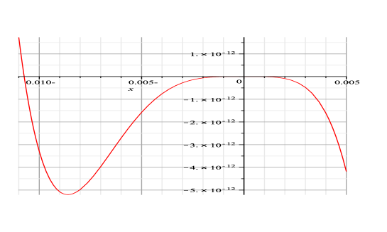
Figure 1. function $H(x)$ with $s=0.647,$  its zero is  $x_{0}=-0.010737...\cdots$ This means the potential $G_{s}$ does not verify condition $(\mathcal{C}_{0})$ when $x\in[-\alpha,\alpha)]$ for $x_{0}<\alpha$

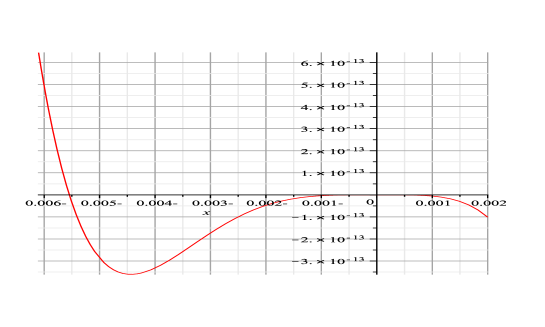
Figure 2. function $H_{1}(x)$ with $s=0.647,$  its zero is  $x_{1}=-0.005545...\cdots$ This means the potential $G_{s}$ does not verify condition $(\mathcal{C}_{1})$when $x\in[-\alpha,\alpha)]$ for $x_{1}<\alpha$

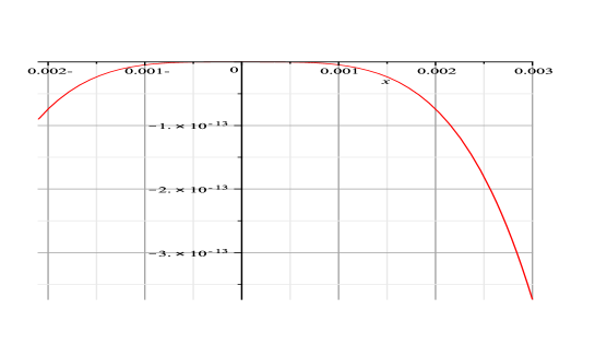
Figure 3. function $H_{2}(x)$ with $s=0.647.$   $H_{2}(x)<0$ for $x\in[-\alpha,\alpha]$ and $x\neq 0.$, here $\alpha=0.04\cdots$ This means $(\mathcal{C}_{2})$ can be satisfied

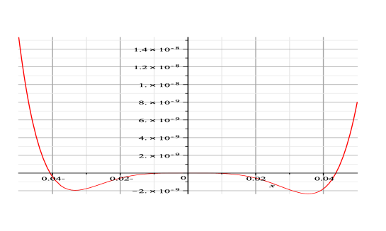
Figure 4. function $H_{2}(x)$ with $s=0.647.$   $H_{2}(x)$ has 2 zeros:      $\alpha_{1}=-0.040743..$ and $\alpha_{2}=0.043699...$ This means the potential $G_{s}$ should verify condition $(\mathcal{C}_{2}),$ for $x\in[-\alpha,\alpha]$. So the period $T(c)$ is decreasing for $0<c<\bar{c}$

4. Appendice: Maple computation details

$>$	eg:=(((x+s)/2)*sinh(2*x)-(cosh(2*x)-1)/4)/s :
$>$	g:=unapply(eg,s,x); # function $g_{s}$
$>$	eG:=int(eg,x)-1/4:G:=unapply(eG,s,x); # primitive of $g_{s}$
$>$	eg1:=diff(eg,x) : g1:=unapply(eg1,s,x); # first derivated of $g_{s}$
$>$	eg2:=diff(eg1,x) : g2:=unapply(eg2,s,x); # second derivated of $g_{s}$
$>$	eg3:=diff(eg2,x) : g3:=unapply(eg3,s,x); # third derivated of $g_{s}$
$>$	eg4:=diff(eg3,x) : g4:=unapply(eg4,s,x); # fourth derivated of $g_{s}$
$>$	.
$>$	.
$>$	.
$>$	fsolve(H(.647, x), x = -0.15e-1 .. -0.1e-2)
-0.01073718589
$>$	fsolve(H1(.647, x), x = -0.15e-1 .. -0.1e-2)
-0.005545373709
$>$	fsolve(H2(.647, x), x = -0.5e-1 .. -0.4e-1)
-0.04074327315
$>$	fsolve(H2(.647, x), x = 0.4e-1 .. 0.5e-1)
0.04369965656

Coefficients of $g_{s}$

Let us write

$$g(x)=x+\frac{a_{2}}{2}x^{2}+\frac{a_{3}}{6}x^{3}+\frac{a_{4}}{24}x^{4}+\frac{a_{5}}{120}x^{5}+....$$

and

$$G=\frac{1}{2}x^{2}+\frac{a_{2}}{6}x^{3}+\frac{a_{3}}{24}x^{4}+...,\ f(G)=b_{0}+b_{1}G+\frac{b_{2}}{2}G^{2}+...$$

By identifying the coefficients we find after simplification

$${\mathit{a}_{3}}=5/3\,{{\mathit{a}_{2}}}^{2},\quad{\mathit{a}_{5}}=-{\frac{140}{9}}\,{{\mathit{a}_{2}}}^{4}+7\,{\mathit{a}_{2}}\,{\mathit{a}_{4}}\quad{\mathit{b}_{0}}=-1/3\,{\mathit{a}_{2}},$$

We thus obtain the first coefficients of the function $f$

$${\mathit{b}_{1}}=-1/5\,{\mathit{a}_{4}}+{\frac{7}{9}}\,{{\mathit{a}_{2}}}^{3}$$

$${\mathit{b}_{2}}=-\frac{28550(g^{\prime\prime}(0))^{6}-10320(g^{\prime\prime}(0))^{3}g^{4}(0)+81(g^{4}(0))^{2}+270(g^{\prime\prime}(0))g^{6}(0)}{2025g^{\prime\prime}(0)}$$

Case of $a_{2}=0$

This case is easier than the previous. We find after simplifying

$$a_{3}=a_{5}=0,\quad a_{7}=(63/5)a_{4}^{2},\quad a_{9}=66a_{6}a_{4}$$

Then it yields the first coefficients of $f$

$$b_{0}=0,\quad b_{1}=-(1/5)a_{4},\quad b_{2}=-(1/42)a_{6},$$

$$b_{3}=-(1/810)a_{8},\quad b_{4}=-(1/27720)a_{10}+(13/600)a_{4}^{3},$$

References

[1]  A.R. Chouikha  Period function and characterizations of Isochronous potentials arXiv:1109.4611, (2011).

[2]  A.R. Chouikha  Monotonicity of the period function for some planar differential systems, I. Conservative and quadratic systems  Applic. Math., 32, no. 3, p. 305-325, (2005).

[3]  A.R. Chouikha and F. Cuvelier  Remarks on some monotonicity conditions for the period function Applic. Math., 26, no. 3, p. 243-252, (1999).

[4]  S.N. Chow and D. Wang  On the monotonicity of the period function of some second order equations Casopis Pest. Mat. 111, p. 14-25, (1986).

[5] L.D. Landau E.M. Lifschitz  Mechanics, Course of Theorical Physics Vol 1, Pergamon Press, Oxford, (1960).

[6]  Z. Opial  Sur les p riodes des solutions de l’ quation diff rentielle  $x^{\prime\prime}+g(x)=0$  Ann. Polon. Math., 10, (1961), 49-72.

[7]  F. Rothe  Remarks on periods of planar Hamiltonian systems.  SIAM J. Math. Anal., 24, p.129-154, (1993).

[8]  R. Schaaf  A class of Hamiltonian systems with increasing periods  J. Reine Angew. Math., 363, p. 96-109, (1985).