Averaging operators over nondegenerate quadratic surfaces in finite fields

Abstract.

We study mapping properties of the averaging operator related to the variety $V=\{x\in\mathbb{F}_{q}^{d}:Q(x)=0\},$ where $Q(x)$ is a nondegenerate quadratic polynomial over a finite field $\mathbb{F}_{q}$ with $q$ elements. This paper is devoted to eliminating the logarithmic bound appearing in the paper [5]. As a consequence, we settle down the averaging problems over the quadratic surfaces $V$ in the case when the dimensions $d\geq 4$ are even and $V$ contains a $d/2$-dimensional subspace.

1. Introduction

Let $V\subset\mathbb{R}^{d}$ be a smooth hypersurface and $d\sigma$ a smooth, compactly supported surface measure on $V.$ An averaging operator $A$ over $V$ is given by

$$Af(x)=f\ast d\sigma(x)=\int_{V}f(x-y)d\sigma(y)$$

where $f$ is a complex valued function on $\mathbb{R}^{d}.$ In this Euclidean setting, the averaging problem is to determine the optimal range of exponents $1\leq p,r\leq\infty$ such that

(1.1) $$\|f\ast d\sigma\|_{L^{r}(\mathbb{R}^{d})}\leq C_{p,r,d}\|f\|_{L^{p}(\mathbb{R}^{d})},~{}~{}f\in\mathcal{S}(\mathbb{R}^{d})$$

where $\mathcal{S}(\mathbb{R}^{d})$ denotes the space of Schwartz functions. When $V$ is the unit sphere $\mathbb{S}^{d-1},$ this problem is closely related to regularity estimates of the solutions to the wave equation at time $t=1$, and it was studied by R.S. Strichartz [12]. It is well known that $L^{p}-L^{r}$ averaging results can be obtained by the decay estimates of the Fourier transform of the surface measure $d\sigma$ on $V$. For instance, if $|\widehat{d\sigma}(\xi)|=\left|\int_{V}e^{-2\pi ix\cdot\xi}d\sigma(x)\right|\lesssim(1+|\xi|)^{-\alpha}$ for some $\alpha>0$, then the averaging inequality (1.1) holds whenever

$$1\leq p\leq 2,\quad\frac{1}{p}-\frac{1}{2}\leq\frac{1}{2}\left(\frac{\alpha}{\alpha+1}\right),~{}~{}\mbox{and}~{}~{}r=p^{\prime},$$

where $p^{\prime}$ denotes the exponent conjugate to $p$ (see [6, 11]). Thus, if $|\widehat{d\sigma}(\xi)|\lesssim(1+|\xi|)^{-(d-1)/2}$ and $(1/p,1/r)=(d/(d+1),1/(d+1)),$ then the averaging estimate (1.1) holds. Since $L^{1}-L^{1}$ and $L^{\infty}-L^{\infty}$ estimates are clearly possible, we see from the interpolation theorem that if $|\widehat{d\sigma}(\xi)|\lesssim(1+|\xi|)^{-(d-1)/2},$ then $L^{p}-L^{r}$ estimates hold whenever $(1/p,1/r)$ lies in the triangle $\Delta_{d}$ with vertices $(0,0),(1,1),$ and $(d/(d+1),1/(d+1)).$ Moreover, it is well known that $L^{p}-L^{r}$ estimates are impossible if $(1/p,1/r)$ lies outside of the triangle $\Delta_{d}.$ Such analogous phenomena were also observed in the finite field setting (see, for example, [1, 4, 5]).
On the other hand, if the optimal Fourier decay estimate of the surface measure $d\sigma$ is given by

$$|\widehat{d\sigma}(\xi)|\lesssim(1+|\xi|)^{-\alpha}\quad\mbox{for some}~{}~{}\alpha<(d-1)/2,$$

then it is in general hard to prove sharp averaging results and some technical arguments are required to deal with the case (see [3]). In the finite field case, this was also pointed out by the authors in [1].

As an analogue of Euclidean averaging problems, Carbery, Stones, and Wright [1] initially introduced and studied the averaging problem in finite fields and the author with Shen has recently investigated the averaging problem over homogeneous varieties. In this introduction, we shortly review notation and definitions for averaging problems in the finite field setting and readers are referred to [5] for further information and motivation on the averaging problem. Let $\mathbb{F}_{q}^{d}$ be a $d$-dimensional vector space over a finite field $\mathbb{F}_{q}$ with $q$ elements. We endow the space $\mathbb{F}_{q}^{d}$ with a normalized counting measure $``dx"$. Let $V\subset\mathbb{F}_{q}^{d}$ be an algebraic variety. Then a normalized surface measure $\sigma$ supported on $V$ can be defined by the relation

$$\int f(x)~{}d\sigma(x)=\frac{1}{|V|}\sum_{x\in V}f(x)$$

where $|V|$ denotes the cardinality of $V$ (see [9]). An averaging operator $A$ can be defined by

$$Af(x)=f\ast d\sigma(x)=\int f(x-y)~{}d\sigma(y)=\frac{1}{|V|}\sum_{y\in V}f(x-y)$$

where both $f$ and $Af$ are functions on $(\mathbb{F}_{q}^{d},dx).$ In this setting the averaging problem over $V$ is to determine $1\leq p,r\leq\infty$ such that

(1.2) $$\|Af\|_{L^{r}(\mathbb{F}_{q}^{d},dx)}\leq C\|f\|_{L^{p}(\mathbb{F}_{q}^{d},dx)},$$

where the constant $C>0$ is independent of functions $f$ and $q$, the cardinality of the underlying finite field $\mathbb{F}_{q}.$

Definition 1.1.

Let $1\leq p,r\leq\infty.$ We denote by $A(p\to r)\lesssim 1$ to indicate that the averaging inequality (1.2) holds.

The main purpose of this paper is to obtain the complete $L^{p}-L^{r}$ estimates of the averaging operators over varieties determined by nondegenerate quadratic form over $\mathbb{F}_{q}$. Let $Q(x)\in\mathbb{F}_{q}[x_{1},\dots,x_{d}]$ be a nondegenerate quadratic form. Define a variety

$$S=\{x\in\mathbb{F}_{q}^{d}:Q(x)=0\}.$$

We shall name this kind of varieties as a nondegenerate quadratic surface in $\mathbb{F}_{q}^{d}.$ Since $Q(x)$ is a nondegenerate quadratic form, it can be transformed into a diagonal form $a_{1}x_{1}^{2}+\dots+a_{d}x_{d}^{2}$ with $a_{j}\neq 0$ by means of a linear substitution (see [8]). Therefore, we may assume that any nondegenerate quadratic surface can be written by the form

(1.3) $$S=\{x\in\mathbb{F}_{q}^{d}:a_{1}x_{1}^{2}+\cdots+a_{d}x_{d}^{2}=0\}$$

where $a_{j}\in\mathbb{F}_{q}\setminus\{0\},j=1,\dots,d.$ The necessary conditions for the averaging estimates over $S$ were given in [1, 5]. In fact, $A(p\to r)\lesssim 1$ only if $(1/p,1/r)$ lies in the convex hull of $(0,0),(0,1),(1,1),$ and $(d/(d+1),1/(d+1)).$ It is known from [5] that this necessary conditions for $A(p\to r)\lesssim 1$ are sufficient conditions if the dimension $d\geq 3$ is odd. On the other hand, it was observed in [5] that if $d\geq 4$ is even and $S$ contains a subspace $H$ with $|H|=q^{d/2},$ then $A(p\to r)\lesssim 1$ only if $(1/p,1/r)$ lies in the convex hull of

(1.4) $$(0,0),(0,1),(1,1),\left(\frac{d^{2}-2d+2}{d(d-1)},~{}\frac{1}{d-1}\right),~{}~{}\mbox{and}~{}~{}\left(\frac{d-2}{d-1},~{}\frac{d-2}{d(d-1)}\right).$$

In this paper we show that (1.4) is also the sufficient conditions for $A(p\to r)\lesssim 1$ in the specific case when the variety $S$ contains $d/2$-dimensional subspace with $d\geq 4$ even. See Figure 1.

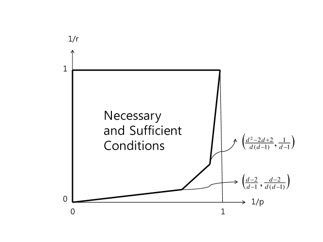
Figure 1. Necessary and Sufficient Conditions for $A(p\to r)\lesssim 1$ in the case that $d\geq 4$ is even and $S$ contains a $d/2$-dimensional subspace

1.1. Statement of main result

Theorem 1.2.

Let $d\sigma$ be the normalized surface measure on the nondegenerate quadratic surface $S\subset\mathbb{F}_{q}^{d},$ as defined in (1.3). Suppose that $d\geq 4$ is an even integer and $S$ contains a $d/2$-dimensional subspace. Then $A(p\to r)\lesssim 1$ if and only if $(1/p,1/r)$ lies in the convex hull of

$$(0,0),(0,1),(1,1),\left(\frac{d^{2}-2d+2}{d(d-1)},~{}\frac{1}{d-1}\right),~{}~{}\mbox{and}~{}~{}\left(\frac{d-2}{d-1},~{}\frac{d-2}{d(d-1)}\right).$$

Remark 1.3.

If the dimension $d\geq 4$ is even, then the diagonal entries $a_{j}$ can be properly chosen so that $S$ contains a $d/2$-dimensional subspace $H.$ Such an example is essentially the following one (see Theorem 4.5.1 of [10]): $S=\{x\in\mathbb{F}_{q}^{d}:\sum_{k=1}^{d}(-1)^{k+1}x_{k}^{2}=0\}$ and $H=\{(t_{1},t_{1},t_{2},t_{2},\dots,t_{d/2},t_{d/2})\in\mathbb{F}_{q}^{d}:t_{1},t_{2},\dots,t_{d/2}\in\mathbb{F}_{q}\}.$

Remark 1.4.

From the observation (1.4), we only need to prove the “ if ” part of Theorem 1.2. Since $dx$ is the normalized counting measure on $\mathbb{F}_{q}^{d}$, it follows from Young’s inequality that $A(p\to r)\lesssim 1$ for $1\leq r\leq p\leq\infty.$ Thus, by duality and the interpolation theorem, it will be enough to prove that

(1.5) $$\|f\ast d\sigma\|_{L^{d-1}(\mathbb{F}_{q}^{d},dx)}\lesssim\|f\|_{L^{d(d-1)/(d^{2}-2d+2)}(\mathbb{F}_{q}^{d},dx)}~{}~{}\mbox{for all functions}~{}~{}f~{}~{}\mbox{on}~{}~{}\mathbb{F}_{q}^{d}.$$

The authors in [5] showed that this inequality holds for all characteristic functions on subsets of $\mathbb{F}_{q}^{d}.$ Here, we improve upon their work by obtaining the strong-type estimate.

1.2. Outline of this paper

In the remaining parts of this paper, we focus on providing the detail proof of Theorem 1.2. In Section 2, we review the Fourier analysis in finite fields and prove key lemmas which are essential in proving our main theorem. The proof of Theorem 1.2 for even dimensions $d\geq 6$ will be completed in Section 3. Namely, when $d\geq 6$ is any even integer, the inequality (1.5) will be proved in Section 3. In the final section, we finish the proof of Theorem 1.2 by proving the inequality (1.5) for $d=4.$

2. key lemmas

In this section we drive key lemmas which play a crucial role in proving Theorem 1.2. We begin by reviewing the Discrete Fourier analysis and readers can be reffered to [5] for more information on it. Let $\mathbb{F}_{q}$ be a finite field with $q$ elements. Throughout this paper, we assume that $q$ is a power of odd prime so that the characteristic of $\mathbb{F}_{q}$ is greater than two. We denote by $\chi$ a nontrivial additive character of $\mathbb{F}_{q}.$ Recall that the orthogonality relation of the canonical additive character $\chi$ says that

$$\sum_{x\in\mathbb{F}_{q}^{d}}\chi(m\cdot x)=\left\{\begin{array}[]{ll}0&\mbox{if}~{}~{}m\neq(0,\dots,0)\\ q^{d}&\mbox{if}~{}~{}m=(0,\dots,0),\end{array}\right.$$

where $\mathbb{F}_{q}^{d}$ denotes the $d$-dimensional vector space over $\mathbb{F}_{q}$ and $m\cdot x$ is the usual dot-product notation. Denote by $(\mathbb{F}_{q}^{d},dx)$ the vector space over $\mathbb{F}_{q}$, endowed with the normalized counting measure $``dx".$ Its dual space will be denoted by $(\mathbb{F}_{q}^{d},dm)$ and we endow it with a counting measure $``dm".$ If $f:(\mathbb{F}_{q}^{d},dx)\rightarrow\mathbb{C},$ then the Fourier transform of the function $f$ is defined on $(\mathbb{F}_{q}^{d},dm)$:

$$\widehat{f}(m)=\int_{\mathbb{F}_{q}^{d}}f(x)\chi(-x\cdot m)~{}dx=\frac{1}{q^{d}}\sum_{x\in\mathbb{F}_{q}^{d}}f(x)\chi(-x\cdot m)\quad\mbox{for}~{}~{}m\in\mathbb{F}_{q}^{d}.$$

We also recall the Plancherel theorem:

$$\sum_{m\in\mathbb{F}_{q}^{d}}|\widehat{f}(m)|^{2}=\frac{1}{q^{d}}\sum_{x\in\mathbb{F}_{q}^{d}}|f(x)|^{2}.$$

Throughout this paper, we identify the set $E\subset\mathbb{F}_{q}^{d}$ with the characteristic function on the set $E.$ We denote by $(d\sigma)^{\vee}$ the inverse Fourier transform of the normalized surface measure $d\sigma$ on $S$ in (1.3) . Recall that

$$(d\sigma)^{\vee}(m)=\int_{S}\chi(m\cdot x)~{}d\sigma(x)=\frac{1}{|S|}\sum_{x\in S}\chi(m\cdot x).$$

2.1. Gauss sums and estimates of $(d\sigma)^{\vee}$

Let $\eta$ denote the quadratic character of ${\mathbb{F}_{q}}.$ For each $t\in{\mathbb{F}_{q}},$ the Gauss sum $G_{t}(\eta,\chi)$ is defined by

$$G_{t}(\eta,\chi)=\sum_{s\in{\mathbb{F}_{q}}\setminus\{0\}}\eta(s)\chi(ts).$$

The absolute value of the Gauss sum is given as follows (see [8, 2]):

$$|G_{t}(\eta,\chi)|=\left\{\begin{array}[]{ll}q^{\frac{1}{2}}&\mbox{if}~{}~{}t\neq 0\\ 0&\mbox{if}~{}~{}t=0,\end{array}\right..$$

It turns out that the inverse Fourier transform of $d\sigma$ can be written in terms of the Gauss sum. The following was given in Lemma 4.1 of [5].

Lemma 2.1.

Let $S$ be the variety in $\mathbb{F}_{q}^{d}$ as defined in (1.3), and let $d\sigma$ be the normalized surface measure on $S.$ If $d\geq 2$ is even, then we have

$$(d\sigma)^{\vee}(m)=\left\{\begin{array}[]{ll}q^{d-1}|S|^{-1}+\frac{G_{1}^{d}}{|S|}(1-q^{-1})\eta(a_{1}\cdots a_{d})&\mbox{if}~{}~{}m=(0,\dots,0)\\ \frac{G_{1}^{d}}{|S|}(1-q^{-1})\eta(a_{1}\cdots a_{d})&\mbox{if}~{}~{}m\neq(0,\dots,0),~{}\frac{m_{1}^{2}}{a_{1}}+\cdots+\frac{m_{d}^{2}}{a_{d}}=0\\ -\frac{G_{1}^{d}}{q|S|}\eta(a_{1}\cdots a_{d})&\mbox{if}~{}~{}\frac{m_{1}^{2}}{a_{1}}+\cdots+\frac{m_{d}^{2}}{a_{d}}\neq 0.\end{array}\right.$$

Here and throughout this paper we denote by $\eta$ the quadratic character of ${\mathbb{F}_{q}}$ and we write $G_{1}$ for the Gauss sum $G_{1}(\eta,\chi).$

Lemma 2.1 yields the following corollary.

Corollary 2.2.

Let $S$ be the variety in $\mathbb{F}_{q}^{d}$ as defined in (1.3) and let $d\sigma$ be the normalized surface measure on $S.$ If $d\geq 4$ is even, then we have

(2.1) $$|S|=q^{d-1}+G_{1}^{d}(1-q^{-1})\eta(a_{1}\cdots a_{d})\sim q^{d-1},$$

and

(2.2) $$|(d\sigma)^{\vee}(m)|\sim\left\{\begin{array}[]{ll}q^{-\frac{(d-2)}{2}}&\mbox{if}~{}~{}m\neq(0,\dots,0),~{}\frac{m_{1}^{2}}{a_{1}}+\cdots+\frac{m_{d}^{2}}{a_{d}}=0\\ q^{-\frac{d}{2}}&\mbox{if}~{}~{}\frac{m_{1}^{2}}{a_{1}}+\cdots+\frac{m_{d}^{2}}{a_{d}}\neq 0.\end{array}\right.$$

Proof.

By the definition of $(d\sigma)^{\vee}(0,\ldots,0)$, it is clear that $(d\sigma)^{\vee}(0,\ldots,0)=1.$ Comparison with Lemma 2.1 shows that

$$|S|=q^{d-1}+G_{1}^{d}(1-q^{-1})\eta(a_{1}\cdots a_{d}).$$

Since $|G_{1}|=q^{1/2}$, it follows that $|S|\sim q^{d-1}$ for $d\geq 4$ even. This proves (2.1). The inequality (2.2) follows immediately from Lemma 2.1 because $|G_{1}|=q^{1/2}$ and $|S|\sim q^{d-1}$ for $d\geq 4$ even. ∎

Remark 2.3.

It is clear from (2.2) that if $d\geq 4$ is even and $S$ is any nondegenerate quadratic surface in $\mathbb{F}_{q}^{d},$ then

(2.3) $$|(d\sigma)^{\vee}(m)|=\left|\frac{1}{|S|}\sum_{x\in S}\chi(m\cdot x)\right|\sim\frac{1}{q^{d-1}}\left|\sum_{x\in S}\chi(m\cdot x)\right|\lesssim q^{-\frac{(d-2)}{2}}~{}~{}\mbox{for}~{}~{}m\in\mathbb{F}_{q}^{d}\setminus\{(0,\dots,0)\}.$$

2.2. Bochner-Riesz kernel

Recall that $d\sigma$ is the normalized surface measure on the nondegenerate quadratic surface $S$ . In the finite field setting, the Bochner-Riesz kernel $K$ is a function on $(\mathbb{F}_{q}^{d},dm)$ and it satisfies that $K=(d\sigma)^{\vee}-\delta_{0}.$ Recall that $dm$ denotes the counting measure on $\mathbb{F}_{q}^{d}.$ Notice that $K(m)=0$ if $m=(0,\ldots,0)$, and $K(m)=(d\sigma)^{\vee}(m)$ otherwise. Also observe that

$$d\sigma=\widehat{K}+\widehat{\delta_{0}}=\widehat{K}+1.$$

Here, the last equality follows because $\delta_{0}$ is defined on the vector space with the counting measure $dm,$ and its Fourier transform $\widehat{\delta_{0}}$ is defined on the dual space with the normalized counting measure $dx.$ More precisely, if $x\in(\mathbb{F}_{q}^{d},dx),$ then

$$\widehat{\delta_{0}}(x)=\int_{m\in\mathbb{F}_{q}^{d}}\chi(-m\cdot x)\delta_{0}(m)~{}dm=\sum_{m\in\mathbb{F}_{q}^{d}}\chi(-m\cdot x)\delta_{0}(m)=1.$$

Our main lemma is as follows.

Lemma 2.4.

Suppose that $d\geq 6$ is even. Then, for every $E\subset\mathbb{F}_{q}^{d},$ we have

(2.4) $$\|E\ast\widehat{K}\|_{L^{\frac{d-1}{2}}(\mathbb{F}_{q}^{d},dx)}\lesssim\left\{\begin{array}[]{ll}q^{\frac{-d^{2}+2d-3}{d-1}}|E|^{\frac{d-3}{d-1}}&\mbox{if}~{}~{}1\leq|E|\leq q^{\frac{d-2}{2}}\\ q^{\frac{-d^{2}+d-1}{d-1}}|E|&\mbox{if}~{}~{}q^{\frac{d-2}{2}}\leq|E|\leq q^{\frac{d}{2}}\\ q^{-d+1}|E|^{\frac{d-3}{d-1}}&\mbox{if}~{}~{}q^{\frac{d}{2}}\leq|E|\leq q^{d}.\end{array}\right.$$

where $K$ is the Bochner-Riesz kernel. On the other hand, for every $E\subset\mathbb{F}_{q}^{4},$ it follows that

(2.5) $$\|E\ast\widehat{K}\|_{L^{6}(\mathbb{F}_{q}^{4},dx)}\lesssim\left\{\begin{array}[]{ll}q^{-\frac{19}{6}}|E|^{\frac{5}{6}}&\mbox{if}~{}~{}1\leq|E|\leq q\\ q^{-\frac{10}{3}}|E|&\mbox{if}~{}~{}q\leq|E|\leq q^{2}\\ q^{-3}|E|^{\frac{5}{6}}&\mbox{if}~{}~{}q^{2}\leq|E|\leq q^{4}.\end{array}\right.$$

Proof.

Using the interpolation theorem, it suffices to prove that the following two inequalities hold for all d$\geq 4$ even:

(2.6) $$\|E\ast\widehat{K}\|_{L^{\infty}(\mathbb{F}_{q}^{d},dx)}\lesssim q^{-d+1}|E|$$

and

(2.7) $$\|E\ast\widehat{K}\|_{L^{2}(\mathbb{F}_{q}^{d},dx)}\lesssim\left\{\begin{array}[]{ll}q^{\frac{-2d+1}{2}}|E|^{\frac{1}{2}}&\mbox{if}~{}~{}1\leq|E|\leq q^{\frac{d-2}{2}}\\ q^{\frac{-5d+4}{4}}|E|&\mbox{if}~{}~{}q^{\frac{d-2}{2}}\leq|E|\leq q^{\frac{d}{2}}\\ q^{-d+1}|E|^{\frac{1}{2}}&\mbox{if}~{}~{}q^{\frac{d}{2}}\leq|E|\leq q^{d}.\end{array}\right.$$

The estimate (2.6) can be obtained by applying Young’s inequality. In fact, we see that

$$\|E\ast\widehat{K}\|_{L^{\infty}(\mathbb{F}_{q}^{d},dx)}\leq\|\widehat{K}\|_{L^{\infty}(\mathbb{F}_{q}^{d},dx)}\|E\|_{L^{1}(\mathbb{F}_{q}^{d},dx)}.$$

Since $\|\widehat{K}\|_{L^{\infty}(\mathbb{F}_{q}^{d},dx)}\lesssim q$ and $\|E\|_{L^{1}(\mathbb{F}_{q}^{d},dx)}=q^{-d}|E|,$ the inequality (2.6) is established. To prove the inequality (2.7), first use the Plancherel theorem. It follows that

$$\|E\ast\widehat{K}\|^{2}_{L^{2}(\mathbb{F}_{q}^{d},dx)}=\|\widehat{E}K\|^{2}_{L^{2}(\mathbb{F}_{q}^{d},dm)}.$$

Now, we recall that $dx$ is the normalized counting measure but $dm$ is the counting measure. Thus, the expression above is given by

$$\sum_{m\in\mathbb{F}_{q}^{d}}|\widehat{E}(m)|^{2}|K(m)|^{2}= \sum_{m\neq(0,\dots,0)}|\widehat{E}(m)|^{2}|(d\sigma)^{\vee}(m)|^{2}$$

$$\sim\frac{1}{q^{d-2}}\sum_{\begin{subarray}{c}m\neq(0,\dots,0):\\ \frac{m_{1}^{2}}{a_{1}}+\cdots+\frac{m_{d}^{2}}{a_{d}}=0\end{subarray}}|\widehat{E}(m)|^{2}+\frac{1}{q^{d}}\sum_{\begin{subarray}{c}m\neq(0,\dots,0):\\ \frac{m_{1}^{2}}{a_{1}}+\cdots+\frac{m_{d}^{2}}{a_{d}}\neq 0\end{subarray}}|\widehat{E}(m)|^{2}=\mbox{I}+\mbox{II},$$

where the first line and the second line follow from the definition of $K$ and the inequality (2.2) in Corollary 2.2, respectively. Applying the Plancherel theorem, it is clear that

(2.8) $$\mbox{II}\leq\frac{1}{q^{d}}\sum_{m\in\mathbb{F}_{q}^{d}}|\widehat{E}(m)|^{2}=q^{-2d}|E|.$$

In order to obtain a good upper bound of I, we shall conduct two different estimates on $\mbox{I}.$ First, the Plancherel theorem yields

(2.9) $$\mbox{I}\leq\frac{1}{q^{d-2}}\sum_{m\in\mathbb{F}_{q}^{d}}|\widehat{E}(m)|^{2}=\frac{|E|}{q^{2d-2}}.$$

On the other hand, it follows that

$$\mbox{I}\leq\frac{1}{q^{d-2}}\sum_{\frac{m_{1}^{2}}{a_{1}}+\cdots+\frac{m_{d}^{2}}{a_{d}}=0}|\widehat{E}(m)|^{2}=\frac{1}{q^{3d-2}}\sum_{\frac{m_{1}^{2}}{a_{1}}+\cdots+\frac{m_{d}^{2}}{a_{d}}=0}\sum_{x,y\in E}\chi(-m\cdot(x-y)).$$

Now, let $S_{a}=\{m\in\mathbb{F}_{q}^{d}:\frac{m_{1}^{2}}{a_{1}}+\cdots+\frac{m_{d}^{2}}{a_{d}}=0\}$ which is also a nondegenerate quadratic surface with $|S_{a}|\sim q^{d-1}.$ Then the expression above can be written by

$$\frac{1}{q^{3d-2}}\sum_{x,y\in E:x=y}|S_{a}|+\frac{1}{q^{3d-2}}\sum_{x,y\in E:x\neq y}\left(\sum_{m\in S_{a}}\chi(-m\cdot(x-y))\right).$$

Now, we see from (2.3) that if $x\neq y$, then $\left|\sum_{m\in S_{a}}\chi(-m\cdot(x-y))\right|\lesssim q^{\frac{d}{2}}.$ Thus, we obtain that

$$\mbox{I}\lesssim q^{-2d+1}|E|+q^{\frac{-5d+4}{2}}|E|^{2}.$$

Combining this with the inequality (2.9) gives

$$\mbox{I}\lesssim\min\left(\frac{|E|}{q^{2d-2}},~{}q^{-2d+1}|E|+q^{\frac{-5d+4}{2}}|E|^{2}\right).$$

In conjunction with the inequality (2.8), this shows that

$$\|E\ast\widehat{K}\|^{2}_{L^{2}(\mathbb{F}_{q}^{d},dx)}\lesssim\min\left(\frac{|E|}{q^{2d-2}},~{}q^{-2d+1}|E|+q^{\frac{-5d+4}{2}}|E|^{2}\right)~{}+q^{-2d}|E|.$$

Since $(\alpha+\beta)^{1/2}\sim\alpha^{1/2}+\beta^{1/2}$ for $\alpha,\beta\geq 0$, it also follows that

$$\|E\ast\widehat{K}\|_{L^{2}(\mathbb{F}_{q}^{d},dx)}\lesssim\min\left(q^{-d+1}|E|^{\frac{1}{2}},~{}q^{\frac{-2d+1}{2}}|E|^{\frac{1}{2}}+q^{\frac{-5d+4}{4}}|E|\right)~{}+q^{-d}|E|^{\frac{1}{2}}.$$

A direct computation shows that this implies the inequality (2.7). We complete the proof of Lemma 2.4.

∎

3. Proof of Theorem 1.2 for $d\geq 6$

In this section we provide the complete proof of Theorem 1.2 in the case that $d\geq 6$ is even. The proof for $d=4$ shall be independently given in the following section. The main reason is as follows. Lemma 2.4 shall be used to prove Theorem 1.2. If $d\geq 6$ is even, then we have seen that the inequality (2.4) of Lemma 2.4 follows by interpolating (2.6) and (2.7). However, if $d$ is four, then such an interpolation is too meaningless to assert that (2.4) holds for $d=4.$ As an alternative approach, the inequality (2.5) of Lemma 2.4 shall be applied to complete the proof for $d=4.$ In this case we need more delicate estimates.

Now we start proving Theorem 1.2 for $d\geq 6$ even. As mentioned in Remark 1.4, it is enough to prove the following statement.

Theorem 3.1.

Let $S$ be the variety in $\mathbb{F}_{q}^{d}$ as defined in (1.3). If $d\geq 6$ is even, then we have

$$\|f\ast d\sigma\|_{L^{r}(\mathbb{F}_{q}^{d},dx)}\lesssim\|f\|_{L^{p}(\mathbb{F}_{q}^{d},dx)}~{}~{}\mbox{for all functions}~{}~{}f~{}~{}\mbox{on}~{}~{}\mathbb{F}_{q}^{d},$$

where $(p,r)=\left(\frac{d^{2}-d}{d^{2}-2d+2},d-1\right).$

Proof.

Let $p=\frac{d^{2}-d}{d^{2}-2d+2}$ and $r=d-1.$ We aim to prove that for every complex-valued function $f$ on $\mathbb{F}_{q}^{d},$

$$\|f\ast d\sigma\|_{L^{r}(\mathbb{F}_{q}^{d},dx)}\lesssim\|f\|_{L^{p}(\mathbb{F}_{q}^{d},dx)}=\left(q^{-d}\sum_{x\in\mathbb{F}_{q}^{d}}|f(x)|^{p}\right)^{\frac{1}{p}}.$$

As in [7] we proceed with the proof by decomposing the function $f$ to which the operator is applied into level sets. Without loss of generality, we may assume that $f$ is a nonnegative real-valued function and

$$\sum_{x\in\mathbb{F}_{q}^{d}}|f(x)|^{p}=1.$$

Therefore, we may also assume that

(3.1) $$f=\sum_{k=0}^{\infty}2^{-k}E_{k},$$

where $E_{0},E_{1},\dots$ are disjoint subsets of $\mathbb{F}_{q}^{d}.$ It follows from these assumptions that

(3.2) $$\sum_{j=0}^{\infty}2^{-pj}|E_{j}|=1,$$

and hence for every $j=0,1,\dots,$

(3.3) $$|E_{j}|\leq 2^{pj}.$$

Recall that $d\sigma=\widehat{K}+1$ where $K$ is the Bochner-Riesz kernel. It follows that

$$\|f\ast d\sigma\|_{L^{r}(\mathbb{F}_{q}^{d},dx)}\leq\|f\ast\widehat{K}\|_{L^{r}(\mathbb{F}_{q}^{d},dx)}+\|f\ast 1\|_{L^{r}(\mathbb{F}_{q}^{d},dx)}.$$

Since $r>p$ and $dx$ is the normalized counting measure on $\mathbb{F}_{q}^{d},$ it is clear from Young’s inequality that

$$\|f\ast 1\|_{L^{r}(\mathbb{F}_{q}^{d},dx)}\leq\|f\|_{L^{p}(\mathbb{F}_{q}^{d},dx)}.$$

Therefore, it suffices to prove the following inequality

$$\|f\ast\widehat{K}\|_{L^{r}(\mathbb{F}_{q}^{d},dx)}\lesssim\|f\|_{L^{p}(\mathbb{F}_{q}^{d},dx)}.$$

Since we have assumed that $\sum_{x\in\mathbb{F}_{q}^{d}}|f(x)|^{p}=1$, we see that $\|f\|_{L^{p}(\mathbb{F}_{q}^{d},dx)}=q^{-d/p}.$ Also observe that

$$\|f\ast\widehat{K}\|^{2}_{L^{r}(\mathbb{F}_{q}^{d},dx)}=\|(f\ast\widehat{K})(f\ast\widehat{K})\|_{L^{\frac{r}{2}}(\mathbb{F}_{q}^{d},dx)}.$$

From these observations, our task is to show that

(3.4) $$q^{\frac{2d}{p}}\|(f\ast\widehat{K})(f\ast\widehat{K})\|_{L^{\frac{r}{2}}(\mathbb{F}_{q}^{d},dx)}\lesssim 1.$$

Using (3.1), we see that

$$q^{\frac{2d}{p}}\|(f\ast\widehat{K})(f\ast\widehat{K})\|_{L^{\frac{r}{2}}(\mathbb{F}_{q}^{d},dx)} \leq q^{\frac{2d}{p}}\sum_{k=0}^{\infty}\sum_{j=0}^{\infty}2^{-k-j}\|(E_{k}\ast\widehat{K})(E_{j}\ast\widehat{K})\|_{L^{\frac{r}{2}}(\mathbb{F}_{q}^{d},dx)}$$

$$\lesssim q^{\frac{2d}{p}}q^{-d+1}\sum_{k=0}^{\infty}\sum_{j=k}^{\infty}2^{-k-j}|E_{k}|\|(E_{j}\ast\widehat{K})\|_{L^{\frac{r}{2}}(\mathbb{F}_{q}^{d},dx)},$$

where the last line follows by the symmetry of $k$ and $j,$ and the inequality (2.6). Now, for each $j=0,1,2,\dots,$ we consider the following three sets:

$$J_{1}=\{j:1\leq|E_{j}|\leq q^{\frac{d-2}{2}}\},$$

$$J_{2}=\{j:q^{\frac{d-2}{2}}<|E_{j}|\leq q^{\frac{d}{2}}\},$$

and

$$J_{3}=\{j:q^{\frac{d}{2}}<|E_{j}|\leq q^{d}\}.$$

Since $r/2=(d-1)/2,$ it is clear from (2.4) in Lemma 2.4 that our goal is to prove the following three inequalities:

(3.5) $$A_{1}:=q^{\frac{2d}{p}}q^{-d+1}q^{\frac{-d^{2}+2d-3}{d-1}}\sum_{k=0}^{\infty}\sum_{j=k:j\in J_{1}}^{\infty}2^{-k-j}|E_{k}||E_{j}|^{\frac{d-3}{d-1}}\lesssim 1,$$

(3.6) $$A_{2}:=q^{\frac{2d}{p}}q^{-d+1}q^{\frac{-d^{2}+d-1}{d-1}}\sum_{k=0}^{\infty}\sum_{j=k:j\in J_{2}}^{\infty}2^{-k-j}|E_{k}||E_{j}|\lesssim 1,$$

(3.7) $$A_{3}:=q^{\frac{2d}{p}}q^{-d+1}q^{-d+1}\sum_{k=0}^{\infty}\sum_{j=k:j\in J_{3}}^{\infty}2^{-k-j}|E_{k}||E_{j}|^{\frac{d-3}{d-1}}\lesssim 1.$$

First, we prove that the inequality (3.5) holds. Since $p=\frac{d^{2}-d}{d^{2}-2d+2},$ a direct computation shows that $q^{\frac{2d}{p}}q^{-d+1}q^{\frac{-d^{2}+2d-3}{d-1}}=1.$ Now recall from (3.3) that $|E_{j}|\leq 2^{pj}$ for all $j=0,1,\dots.$ Therefore, it follows that

$$A_{1}\leq\sum_{k=0}^{\infty}\sum_{j=k:j\in J_{1}}^{\infty}2^{-k-j}|E_{k}|2^{\frac{jp(d-3)}{d-1}}\leq\sum_{k=0}^{\infty}2^{-k}|E_{k}|\sum_{j=k}^{\infty}2^{j\left(-1+\frac{p(d-3)}{d-1}\right)}.$$

Since $-1+\frac{p(d-3)}{d-1}=\frac{-d-2}{d^{2}-2d+2}<0$ and the sum over $j$ is a geometric series, we see that $\sum_{j=k}^{\infty}2^{j\left(-1+\frac{p(d-3)}{d-1}\right)}\sim 2^{k\left(-1+\frac{p(d-3)}{d-1}\right)}.$ Thus, the inequality (3.5) is established as follows:

$$A_{1}\lesssim\sum_{k=0}^{\infty}|E_{k}|2^{k\left(-2+\frac{p(d-3)}{d-1}\right)}\leq\sum_{k=0}^{\infty}|E_{k}|2^{-pk}=1,$$

where we used the simple observation that $-2+\frac{p(d-3)}{d-1}<-p,$ and then the assumption $(\ref{as1}).$
Second, we prove that the inequality (3.6) holds. Let $\varepsilon=\frac{2d-4}{d^{2}-d}.$ Since $d\geq 6,$ we see that $0<\varepsilon<1.$ Write $A_{2}$ as follows:

$$A_{2}=q^{\frac{2d}{p}}q^{-d+1}q^{\frac{-d^{2}+d-1}{d-1}}\sum_{k=0}^{\infty}\sum_{j=k:j\in J_{2}}^{\infty}2^{-k-j}|E_{k}||E_{j}|^{1-\varepsilon}|E_{j}|^{\varepsilon}.$$

Since $0<\varepsilon<1,$ we notice from (3.3) that $|E_{j}|^{1-\varepsilon}\leq 2^{p(1-\varepsilon)j}.$ By the definition of the set $J_{2}$, we also see that $|E_{j}|^{\varepsilon}\leq q^{\frac{d\varepsilon}{2}}$ for all $j\in J_{2}.$ Then, we have

$$A_{2} \leq q^{\frac{2d}{p}}q^{-d+1}q^{\frac{-d^{2}+d-1}{d-1}}q^{\frac{d\varepsilon}{2}}\sum_{k=0}^{\infty}\sum_{j=k:j\in J_{2}}^{\infty}2^{-k-j}|E_{k}|2^{p(1-\varepsilon)j}$$

$$\leq q^{\frac{2d}{p}}q^{-d+1}q^{\frac{-d^{2}+d-1}{d-1}}q^{\frac{d\varepsilon}{2}}\sum_{k=0}^{\infty}2^{-k}|E_{k}|\sum_{j=k}^{\infty}2^{j\left(-1+p(1-\varepsilon)\right)}.$$

Notice that $q^{\frac{2d}{p}}q^{-d+1}q^{\frac{-d^{2}+d-1}{d-1}}q^{\frac{d\varepsilon}{2}}=1,$ and the geometric series over $j$ converges to $\sim 2^{k\left(-1+p(1-\varepsilon)\right)}$ because $-1+p(1-\varepsilon)=\frac{-d+2}{d^{2}-2d+2}<0$ for $d\geq 6.$ From this observation and (3.2), the inequality (3.6) follows because we have

$$A_{2}\lesssim\sum_{k=0}^{\infty}|E_{k}|2^{k\left(-2+p(1-\varepsilon)\right)}=\sum_{k=0}^{\infty}|E_{k}|2^{-pk}=1.$$

Finally, we show that the inequality (3.7) holds. As in the proof of the inequality (3.6), we let $0<\delta=\frac{4}{d^{2}-d}<1$ for $d\geq 6.$ The value $A_{3}$ is written by

$$A_{3}=q^{\frac{2d}{p}}q^{-d+1}q^{-d+1}\sum_{k=0}^{\infty}\sum_{j=k:j\in J_{3}}^{\infty}2^{-k-j}|E_{k}||E_{j}|^{\delta+\frac{d-3}{d-1}}|E_{j}|^{-\delta}.$$

Notice from (3.3) that $|E_{j}|^{\delta+\frac{d-3}{d-1}}\leq 2^{p\left(\delta+\frac{d-3}{d-1}\right)j}$ for all $j=0,1,2,\dots.$ By the definition of $J_{3}$, it is easy to notice that $|E_{j}|^{-\delta}\leq q^{\frac{-d\delta}{2}}$ for $j\in J_{3}.$ It therefore follows that

$$A_{3} \leq q^{\frac{2d}{p}}q^{-d+1}q^{-d+1}q^{\frac{-d\delta}{2}}\sum_{k=0}^{\infty}\sum_{j=k:j\in J_{3}}^{\infty}2^{-k-j}|E_{k}|2^{p\left(\delta+\frac{d-3}{d-1}\right)j}$$

$$\leq\sum_{k=0}^{\infty}2^{-k}|E_{k}|\sum_{j=k}^{\infty}2^{\left(-1+p\left(\delta+\frac{d-3}{d-1}\right)\right)j}$$

$$\sim\sum_{k=0}^{\infty}|E_{k}|2^{\left(-2+p\left(\delta+\frac{d-3}{d-1}\right)\right)k}=\sum_{k=0}^{\infty}|E_{k}|2^{-pk}=1,$$

where we used the facts that $q^{\frac{2d}{p}}q^{-d+1}q^{-d+1}q^{\frac{-d\delta}{2}}=1,$ $\left(-1+p\left(\delta+\frac{d-3}{d-1}\right)\right)=\frac{-d+2}{d^{2}-2d+2}<0$ for $d\geq 6,$ and $\left(-2+p\left(\delta+\frac{d-3}{d-1}\right)\right)=-p,$ and then the assumption (3.2) for the last equality. Thus, the inequality (3.7) holds and the proof of Theorem 3.1 is complete.∎

4. Proof of Theorem 1.2 for $d=4$

As observed in Remark 1.4, it amounts to showing the following statement.

Theorem 4.1.

Let $S$ be the variety in $\mathbb{F}_{q}^{4}$ as defined in (1.3). Then, we have

$$\|f\ast d\sigma\|_{L^{3}(\mathbb{F}_{q}^{4},dx)}\lesssim\|f\|_{L^{\frac{6}{5}}(\mathbb{F}_{q}^{4},dx)}~{}~{}\mbox{for all functions}~{}~{}f~{}~{}\mbox{on}~{}~{}\mathbb{F}_{q}^{4}.$$

Proof.

We will proceed by the similar ways as in the previous section. However, the proof of the theorem will be based on (2.5), rather than (2.4) in Lemma 2.4. We begin by recalling from (2.5) and (2.7) that

(4.1) $$\|E\ast\widehat{K}\|_{L^{6}(\mathbb{F}_{q}^{4},dx)}\lesssim\left\{\begin{array}[]{ll}q^{-\frac{19}{6}}|E|^{\frac{5}{6}}&\mbox{if}~{}~{}1\leq|E|\leq q\\ q^{-\frac{10}{3}}|E|&\mbox{if}~{}~{}q\leq|E|\leq q^{2}\\ q^{-3}|E|^{\frac{5}{6}}&\mbox{if}~{}~{}q^{2}\leq|E|\leq q^{4},\end{array}\right.$$

and

(4.2) $$\|E\ast\widehat{K}\|_{L^{2}(\mathbb{F}_{q}^{4},dx)}\lesssim\left\{\begin{array}[]{ll}q^{-\frac{7}{2}}|E|^{\frac{1}{2}}&\mbox{if}~{}~{}1\leq|E|\leq q\\ q^{-4}|E|&\mbox{if}~{}~{}q\leq|E|\leq q^{2}\\ q^{-3}|E|^{\frac{1}{2}}&\mbox{if}~{}~{}q^{2}\leq|E|\leq q^{4}.\end{array}\right.$$

We must show that for all complex-valued functions $f$ on $\mathbb{F}_{q}^{4},$

$$\|f\ast d\sigma\|_{L^{3}(\mathbb{F}_{q}^{4},dx)}\lesssim\|f\|_{L^{\frac{6}{5}}(\mathbb{F}_{q}^{4},dx)}.$$

As noticed in the previous section, it suffices to prove this inequality under the following assumptions:

$$\sum_{x\in\mathbb{F}_{q}^{4}}|f(x)|^{\frac{6}{5}}=1\quad\mbox{and}\quad f=\sum_{k=0}^{\infty}2^{-k}E_{k},$$

where $E_{0},E_{1},\dots$ are disjoint subsets of $\mathbb{F}_{q}^{4}.$ From these assumptions, it is clear that

(4.3) $$\sum_{j=0}^{\infty}2^{-\frac{6j}{5}}|E_{j}|=1\quad\mbox{for all}~{}j=0,1,\dots.$$

This clearly implies that

(4.4) $$|E_{j}|\leq 2^{\frac{6j}{5}}\quad\mbox{for all}~{}j=0,1,\dots.$$

According to (3.4), it is enough to prove that

$$q^{\frac{20}{3}}\|(f\ast\widehat{K})(f\ast\widehat{K})\|_{L^{\frac{3}{2}}(\mathbb{F}_{q}^{4},dx)}\lesssim 1.$$

Since $f=\sum_{k=0}^{\infty}2^{-k}E_{k},$ it is enough to show that

$$q^{\frac{20}{3}}\sum_{k=0}^{\infty}\sum_{j=0}^{\infty}2^{-k-j}\|(E_{k}\ast\widehat{K})(E_{j}\ast\widehat{K})\|_{L^{\frac{3}{2}}(\mathbb{F}_{q}^{4},dx)}\lesssim 1.$$

By the symmetry of $k$ and $j,$ and the Hölder inequality, our task is to prove

$$q^{\frac{20}{3}}\sum_{k=0}^{\infty}\sum_{j=k}^{\infty}2^{-k-j}\|(E_{k}\ast\widehat{K})\|_{L^{6}(\mathbb{F}_{q}^{4},dx)}\|(E_{j}\ast\widehat{K})\|_{L^{2}(\mathbb{F}_{q}^{4},dx)}\lesssim 1.$$

Main steps to prove this inequality are summarized as follows. By considering the sizes of $|E_{k}|$ and $|E_{j}|$, we first decompose $\sum_{k=0}^{\infty}\sum_{j=k}^{\infty}$ as nine parts. Next, using the estimates (4.1),(4.2), (4.4), (4.3), and a convergence property of a geometric series, we show that each part of them is $\lesssim 1,$ which completes the proof of Theorem 4.1. For the sake of completeness, we shall give full details. To do this, let us define the following $9$ sets: for $N=\{0,1,\dots\},$

$$I_{1}=\{(k,j)\in N\times N:k\leq j,~{}1\leq|E_{k}|\leq q,~{}1\leq|E_{j}|\leq q\},$$

$$I_{2}=\{(k,j)\in N\times N:k\leq j,~{}1\leq|E_{k}|\leq q,~{}q<|E_{j}|\leq q^{2}\},$$

$$I_{3}=\{(k,j)\in N\times N:k\leq j,~{}1\leq|E_{k}|\leq q,~{}q^{2}<|E_{j}|\leq q^{4}\},$$

$$I_{4}=\{(k,j)\in N\times N:k\leq j,~{}q<|E_{k}|\leq q^{2},~{}1\leq|E_{j}|\leq q\},$$

$$I_{5}=\{(k,j)\in N\times N:k\leq j,~{}q<|E_{k}|\leq q^{2},~{}q<|E_{j}|\leq q^{2}\},$$

$$I_{6}=\{(k,j)\in N\times N:k\leq j,~{}q<|E_{k}|\leq q^{2},~{}q^{2}<|E_{j}|\leq q^{4}\},$$

$$I_{7}=\{(k,j)\in N\times N:k\leq j,~{}q^{2}<|E_{k}|\leq q^{4},~{}1\leq|E_{j}|\leq q\},$$

$$I_{8}=\{(k,j)\in N\times N:k\leq j,~{}q^{2}<|E_{k}|\leq q^{4},~{}q<|E_{j}|\leq q^{2}\},$$

$$I_{9}=\{(k,j)\in N\times N:k\leq j,~{}q^{2}<|E_{k}|\leq q^{4},~{}q^{2}<|E_{j}|\leq q^{4}\}.$$

4.1. Estimate of the sum over $I_{1}$

It follows from (4.1) and (4.2) that

$$q^{\frac{20}{3}}\sum_{(k,j)\in I_{1}}2^{-k-j}\|(E_{k}\ast\widehat{K})\|_{L^{6}(\mathbb{F}_{q}^{4},dx)}\|(E_{j}\ast\widehat{K})\|_{L^{2}(\mathbb{F}_{q}^{4},dx)}$$

$$\lesssim \sum_{(k,j)\in I_{1}}2^{-k-j}|E_{k}|^{\frac{5}{6}}|E_{j}|^{\frac{1}{2}}\leq\sum_{(k,j)\in I_{1}}2^{-k-j}|E_{k}|2^{\frac{3j}{5}}\quad\mbox{since}\quad|E_{j}|^{\frac{1}{2}}\leq 2^{\frac{3j}{5}}\quad\mbox{by (\ref{size})}$$

$$\leq \sum_{k=0}^{\infty}|E_{k}|2^{-k}\sum_{j=k}^{\infty}2^{-\frac{2j}{5}}\sim\sum_{k=0}^{\infty}|E_{k}|2^{-\frac{7k}{5}}\leq\sum_{k=0}^{\infty}2^{-\frac{6k}{5}}|E_{k}|=1\quad\mbox{by (\ref{one})}.$$

4.2. Estimate of the sum over $I_{2}$

It follows from (4.1) and (4.2) that

$$q^{\frac{20}{3}}\sum_{(k,j)\in I_{2}}2^{-k-j}\|(E_{k}\ast\widehat{K})\|_{L^{6}(\mathbb{F}_{q}^{4},dx)}\|(E_{j}\ast\widehat{K})\|_{L^{2}(\mathbb{F}_{q}^{4},dx)}$$

$$\lesssim q^{-\frac{1}{2}}\sum_{(k,j)\in I_{2}}2^{-k-j}|E_{k}|^{\frac{5}{6}}|E_{j}|\leq q^{-\frac{1}{2}}\sum_{(k,j)\in I_{2}}2^{-j}|E_{j}|\quad\mbox{since}\quad 2^{-k}|E_{k}|^{\frac{5}{6}}\leq 1\quad\mbox{by (\ref{size})}$$

$$\leq \sum_{(k,j)\in I_{2}}2^{-j}|E_{j}|^{\frac{3}{4}}\quad\mbox{since}\quad|E_{j}|^{\frac{1}{4}}\leq q^{\frac{1}{2}}\quad\mbox{for}~{}~{}(k,j)\in I_{2}$$

$$\leq \sum_{k=0}^{\infty}\sum_{j=k}^{\infty}2^{-\frac{j}{10}}\quad\mbox{by (\ref{size})}$$

$$\sim \sum_{k=0}^{\infty}2^{-\frac{k}{10}}\sim 1.$$

4.3. Estimate of the sum over $I_{3}$

It follows from (4.1) and (4.2) that

$$q^{\frac{20}{3}}\sum_{(k,j)\in I_{3}}2^{-k-j}\|(E_{k}\ast\widehat{K})\|_{L^{6}(\mathbb{F}_{q}^{4},dx)}\|(E_{j}\ast\widehat{K})\|_{L^{2}(\mathbb{F}_{q}^{4},dx)}$$

$$\lesssim q^{\frac{1}{2}}\sum_{(k,j)\in I_{3}}2^{-k-j}|E_{k}|^{\frac{5}{6}}|E_{j}|^{\frac{1}{2}}\leq q^{\frac{1}{2}}\sum_{(k,j)\in I_{3}}2^{-j}|E_{j}|^{\frac{1}{2}}\quad\mbox{by (\ref{size})}$$

$$= \sum_{(k,j)\in I_{3}}2^{-j}|E_{j}|^{\frac{3}{4}}q^{\frac{1}{2}}|E_{j}|^{-\frac{1}{4}}<\sum_{(k,j)\in I_{3}}2^{-j}|E_{j}|^{\frac{3}{4}}\quad\mbox{since}\quad q^{2}<|E_{j}|~{}~{}\mbox{for}~{}~{}(k,j)\in I_{3}$$

$$\leq \sum_{k=0}^{\infty}\sum_{j=k}^{\infty}2^{-\frac{j}{10}}\sim\sum_{k=0}^{\infty}2^{-\frac{k}{10}}\sim 1.$$

where (4.4) was also used to obtain the last inequality .

4.4. Estimate of the sum over $I_{4}$

It follows from (4.1) and (4.2) that

$$q^{\frac{20}{3}}\sum_{(k,j)\in I_{4}}2^{-k-j}\|(E_{k}\ast\widehat{K})\|_{L^{6}(\mathbb{F}_{q}^{4},dx)}\|(E_{j}\ast\widehat{K})\|_{L^{2}(\mathbb{F}_{q}^{4},dx)}$$

$$\lesssim q^{-\frac{1}{6}}\sum_{(k,j)\in I_{4}}2^{-k-j}|E_{k}||E_{j}|^{\frac{1}{2}}\leq q^{-\frac{1}{6}}\sum_{(k,j)\in I_{4}}2^{-k}|E_{k}|2^{-j}2^{\frac{3j}{5}}\quad\mbox{by (\ref{size})}$$

$$\leq q^{-\frac{1}{6}}\sum_{k=0}^{\infty}2^{-k}|E_{k}|\sum_{j=k}^{\infty}2^{-\frac{2j}{5}}\sim q^{-\frac{1}{6}}\sum_{k=0}^{\infty}2^{-\frac{7k}{5}}|E_{k}|$$

$$\leq \sum_{k=0}^{\infty}2^{-\frac{6k}{5}}|E_{k}|=1\quad\mbox{by (\ref{one})}.$$

4.5. Estimate of the sum over $I_{5}$

It follows from (4.1) and (4.2) that

$$q^{\frac{20}{3}}\sum_{(k,j)\in I_{5}}2^{-k-j}\|(E_{k}\ast\widehat{K})\|_{L^{6}(\mathbb{F}_{q}^{4},dx)}\|(E_{j}\ast\widehat{K})\|_{L^{2}(\mathbb{F}_{q}^{4},dx)}$$

$$\lesssim q^{-\frac{2}{3}}\sum_{(k,j)\in I_{5}}2^{-k-j}|E_{k}||E_{j}|\leq\sum_{(k,j)\in I_{5}}2^{-k-j}|E_{k}||E_{j}|^{\frac{2}{3}}\quad\mbox{since}~{}~{}|E_{j}|^{\frac{1}{3}}\leq q^{\frac{2}{3}}\quad\mbox{for}~{}~{}(k,j)\in I_{5}$$

$$\leq \sum_{k=0}^{\infty}2^{-k}|E_{k}|\sum_{j=k}^{\infty}2^{-\frac{j}{5}}\sim\sum_{k=0}^{\infty}2^{-\frac{6k}{5}}|E_{k}|=1,$$

where we used (4.4), the convergence of a geometric series, and (4.3) in the last line.

4.6. Estimate of the sum over $I_{6}$

It follows from (4.1) and (4.2) that

$$q^{\frac{20}{3}}\sum_{(k,j)\in I_{6}}2^{-k-j}\|(E_{k}\ast\widehat{K})\|_{L^{6}(\mathbb{F}_{q}^{4},dx)}\|(E_{j}\ast\widehat{K})\|_{L^{2}(\mathbb{F}_{q}^{4},dx)}$$

$$\lesssim q^{\frac{1}{3}}\sum_{(k,j)\in I_{6}}2^{-k-j}|E_{k}||E_{j}|^{\frac{1}{2}}<\sum_{(k,j)\in I_{6}}2^{-k-j}|E_{k}||E_{j}|^{\frac{1}{2}+\frac{1}{6}}\quad\mbox{since}~{}~{}|E_{j}|^{-\frac{1}{6}}<q^{-\frac{1}{3}}\quad\mbox{for}~{}~{}(k,j)\in I_{6}$$

$$\leq \sum_{k=0}^{\infty}2^{-k}|E_{k}|\sum_{j=k}^{\infty}2^{-\frac{j}{5}}\sim\sum_{k=0}^{\infty}2^{-\frac{6k}{5}}|E_{k}|=1,$$

where (4.4), the convergence of a geometric series, and (4.3) were also applied in the last line.

4.7. Estimate of the sum over $I_{7}$

It follows from (4.1) and (4.2) that

$$q^{\frac{20}{3}}\sum_{(k,j)\in I_{7}}2^{-k-j}\|(E_{k}\ast\widehat{K})\|_{L^{6}(\mathbb{F}_{q}^{4},dx)}\|(E_{j}\ast\widehat{K})\|_{L^{2}(\mathbb{F}_{q}^{4},dx)}$$

$$\lesssim q^{\frac{1}{6}}\sum_{(k,j)\in I_{7}}2^{-k-j}|E_{k}|^{\frac{5}{6}}|E_{j}|^{\frac{1}{2}}=q^{\frac{1}{6}}\sum_{(k,j)\in I_{7}}2^{-k-j}|E_{k}||E_{k}|^{-\frac{1}{6}}|E_{j}|^{\frac{1}{2}}$$

$$< q^{\frac{1}{6}-\frac{1}{3}}\sum_{(k,j)\in I_{7}}2^{-k}|E_{k}|2^{-\frac{2j}{5}}\quad\mbox{by observing}\quad|E_{k}|^{-\frac{1}{6}}<q^{-\frac{1}{3}}\quad{for}~{}~{}(k,j)\in I_{7}~{}~{}\mbox{and by (\ref{size})}$$

$$\leq \sum_{k=0}^{\infty}2^{-k}|E_{k}|\sum_{j=k}^{\infty}2^{-\frac{2j}{5}}\sim\sum_{k=0}^{\infty}2^{-\frac{7k}{5}}|E_{k}|\leq\sum_{k=0}^{\infty}2^{-\frac{6k}{5}}|E_{k}|=1.$$

4.8. Estimate of the sum over $I_{8}$

It follows from (4.1) and (4.2) that

$$q^{\frac{20}{3}}\sum_{(k,j)\in I_{8}}2^{-k-j}\|(E_{k}\ast\widehat{K})\|_{L^{6}(\mathbb{F}_{q}^{4},dx)}\|(E_{j}\ast\widehat{K})\|_{L^{2}(\mathbb{F}_{q}^{4},dx)}$$

$$\lesssim q^{-\frac{1}{3}}\sum_{(k,j)\in I_{8}}2^{-k-j}|E_{k}|^{\frac{5}{6}}|E_{j}|=q^{-\frac{1}{3}}\sum_{(k,j)\in I_{8}}2^{-k-j}|E_{k}||E_{j}|^{\frac{2}{3}}|E_{k}|^{-\frac{1}{6}}|E_{j}|^{\frac{1}{3}}$$

$$< \sum_{(k,j)\in I_{8}}2^{-k-j}|E_{k}||E_{j}|^{\frac{2}{3}}\quad\mbox{since}~{}~{}|E_{k}|^{-\frac{1}{6}}<q^{-\frac{1}{3}},\quad|E_{j}|^{\frac{1}{3}}\leq q^{\frac{2}{3}}~{}~{}\mbox{for}~{}~{}(k,j)\in I_{8}$$

$$\leq \sum_{k=0}^{\infty}2^{-k}|E_{k}|\sum_{j=k}^{\infty}2^{-\frac{j}{5}}\sim\sum_{k=0}^{\infty}2^{-\frac{6k}{5}}|E_{k}|=1.$$

4.9. Estimate of the sum over $I_{9}$

It follows from (4.1) and (4.2) that

$$q^{\frac{20}{3}}\sum_{(k,j)\in I_{9}}2^{-k-j}\|(E_{k}\ast\widehat{K})\|_{L^{6}(\mathbb{F}_{q}^{4},dx)}\|(E_{j}\ast\widehat{K})\|_{L^{2}(\mathbb{F}_{q}^{4},dx)}$$

$$\lesssim q^{\frac{2}{3}}\sum_{(k,j)\in I_{9}}2^{-k-j}|E_{k}|^{\frac{5}{6}}|E_{j}|^{\frac{1}{2}}=q^{\frac{2}{3}}\sum_{(k,j)\in I_{9}}2^{-k-j}|E_{k}||E_{j}|^{\frac{1}{2}+\frac{1}{6}}|E_{k}|^{-\frac{1}{6}}|E_{j}|^{-\frac{1}{6}}$$

$$< \sum_{(k,j)\in I_{9}}2^{-k-j}|E_{k}||E_{j}|^{\frac{1}{2}+\frac{1}{6}}\quad\mbox{since}~{}~{}|E_{k}|^{-\frac{1}{6}},|E_{j}|^{-\frac{1}{6}}<q^{-\frac{1}{3}}~{}~{}\mbox{for}~{}~{}(k,j)\in I_{9}$$

$$= \sum_{k=0}^{\infty}2^{-k}|E_{k}|\sum_{j=k}^{\infty}2^{-j}|E_{j}|^{\frac{2}{3}}\leq\sum_{k=0}^{\infty}2^{-k}|E_{k}|\sum_{j=k}^{\infty}2^{-\frac{j}{5}}\sim\sum_{k=0}^{\infty}2^{-\frac{6k}{5}}|E_{k}|=1,$$

where we also used (4.4), the convergence of a geometric series, and (4.3) in the last line. ∎

Acknowledgment : The author would like to thank the referee for his/her valuable comments for developing the final version of this paper.

References

- [1] A. Carbery, B. Stones, and J. Wright, Averages in vector spaces over finite fields, Math. Proc. Camb. Phil. Soc. (2008), 144, 13, 13–27.
- [2] H. Iwaniec and E. Kowalski, Analytic Number Theory, Colloquium Publications, 53 (2004).
- [3] A. Iosevich and E. Sawyer, Sharp estimates for a class of averaging operators, Ann. Inst. Fourier, Grenoble, 46, 5 (1996), 1359–1384.
- [4] D. Koh and C. Shen, Harmonic analysis related to homogeneous varieties in three dimensional vector spaces over finite fields, Canad. J. Math. 64 (2012), 1036-1057.
- [5] D. Koh and C. Shen, Extension and averaging operators for finite fields, Proc. Edinb. Math. Soc., To appear.
- [6] W. Littman, estimates for singular integral operators, Proc. Symp. Pure Math., 23(1973), 479–481.
- [7] A. Lewko and M. Lewko, Endpoint restriction estimates for the paraboloid over finite fields, Proc. Amer. Math. Soc. 140 (2012), 2013-2028.
- [8] R. Lidl and H. Niederreiter, Finite fields, Cambridge University Press, (1997).
- [9] G. Mockenhaupt, and T. Tao, Restriction and Kakeya phenomena for finite fields, Duke Math. J. 121(2004), no. 1, 35–74.
- [10] W. Scharlau, Quadratic forms, Queen’s papers on pure and applied math., no. 22, Queen’s Univ., Kingston, Ontario, 1969.
- [11] E.M.Stein, Harmonic analysis, Princeton University Press, 1993.
- [12] R.S. Strichartz, Convolutions with kernels having singularities on a sphere, Trans. Amer. Math. Soc. 148 (1970), 461–471.