Local Properties of WMAP Cold Spot

Abstract

We investigate the local properties of WMAP Cold Spot (CS) by defining the local statistics: mean temperature, variance, skewness and kurtosis. We find that, compared with the coldest spots in random Gaussian simulations, WMAP CS deviates from Gaussianity at $\sim 99\%$ significant level. In the meanwhile, when compared with the spots at the same position in the simulated maps, the values of local variance and skewness around CS are all systematically larger in the scale of $R>5^{\circ}$, which implies that WMAP CS is a large-scale non-Gaussian structure, rather than a combination of some small structures. This is consistent with the finding that the non-Gaussianity of CS is totally encoded in the WMAP low multipoles. Furthermore, we find that the cosmic texture can excellently explain all the anomalies in these statistics.

1 Introduction

Cosmic Microwave Background (CMB) radiation is one of the most ancient fossils of the Universe. The observations of the NASA Wilkinson Microwave Anisotropy Probe (WMAP) satellite on the CMB temperature and polarization anisotropies have put tight constraints on the cosmological parameters (Komatsu et al., 2011). In addition, some anomalies in CMB field have also been reported soon after the release of the WMAP data (see (Bennett et al., 2011) as a review). Among these, an extremely Cold Spot (CS) centered at Galactic coordinate ($l=209^{\circ}$, $b=-57^{\circ}$) with a characteristic scale about $10^{\circ}$ was detected in the Spherical Mexican Hat Wavelet (SMHW) non-Gaussian analyses (Vielva et al., 2004).

Compared with the distribution derived from the isotropic and Gaussian CMB simulations, due to this CS, the SMHW coefficients of WMAP data have an excess of kurtosis (Cruz et al., 2005). In addition, several non-Gaussian statistics, such as the amplitude and area of the cold spot, the higher criticism and so on, have also been applied to identify this WMAP CS (Cruz et al., 2007a, 2005; Cayon et al., 2005; Naselsky et al., 2010; Zhang & Huterer, 2010; Vielva, 2010). Since then, various alternative explanations for the CS have been proposed, including the possible foregrounds (Cruz et al., 2006; Hansen et al., 2012), Sunyaev-Zeldovich effect (Cruz et al., 2008), the supervoid in the Universe (Inoue & Silk, 2006, 2007; Inoue, 2012), and the cosmic texture (Cruz et al., 2007b, 2008). In order to distinguish different interpretations, some analyses have been carried out, such as the non-Gaussian tests for the different detectors and different frequency channels of WMAP satellite (Vielva et al., 2004; Cruz et al., 2005), the investigation of the NVSS sources (Rudnick et al., 2007; Smith & Huterer, 2010), the survey around the CS with MegaCam on the Canada-France-Hawaii Telescope (Granett et al., 2009), the redshift survey using VIMOS on VLT towards CS (Bremer et al., 2010), and the cross-correlation between WMAP and Faraday depth rotation map (Hansen et al., 2012).

Nearly all the interpretations of CS are related to the local characters of the CMB field, so the studies on the local properties of CS are necessary. In this paper, we shall propose a set of novel non-Gaussian statistics, i.e. the local mean temperature, variance, skewness and kurtosis, to study the local properties of the CMB field. By altering the radium of the cap around CS, we study the local properties of CS at different scales. Compared with the coldest spots in the random Gaussian simulations, we find the local non-Gaussianity of WMAP CS, i.e. it deviates from Gaussianity at $\sim 99\%$ significant level. Furthermore, we find the significant difference between WMAP CS and Gaussian simulations at all the scales $1^{\circ}\leq R\leq 15^{\circ}$.

To study the possible origin of WMAP CS, we have also compared it with the spots at the same position of the simulated Gaussian samples. We find that different from the general properties of the foregrounds, the point sources or various local contaminations, in the small scales the local variance, skewness and kurtosis values of CS are not significantly large, except for its coldness in temperature. However, after the careful comparison with Gaussian simulations, we find that when $R>5^{\circ}$ the local variance and skewness are systematically large. This implies that CS prefers a large-scale non-Gaussian structure. In order to confirm it, we repeat the analyses adopted by many authors, where the statistics of temperature and kurtosis in SMHW domain are used. We apply these analyses to the WMAP data with different $l_{\max}$, and find that nearly all the non-Gaussianities of CS are encoded in the low multipoles $l\leq 40$.

It was claimed that the cosmic texture seemed to be the most promising explanation (Cruz et al., 2007b, 2008), by investigating the temperature and area of CS. In order to check this explanation by our local statistics, we superimpose a similar cosmic texture into the simulated Gaussian samples, and calculate the local statistics of the CMB fields. We find that the excesses of the local statistics of WMAP CS can be excellently explained by this non-Gaussian structure. So our local analyses of the CS supports the cosmic texture explanation.

The rest of the paper is organized as follows: In Section 2, we introduce the WMAP data, which will be used in the analyses. In Section 3, we define the local statistics and apply them to WMAP data. In Section 4, the dependence of the WMAP non-Gaussianities on the value of $l_{\max}$ are studied, which shows that the non-Gaussian signals are all encoded in the low multipoles. Section 5 summarizes the main results of this paper.

2 WMAP data and simulations

In our analyses, we shall use the WMAP data including the VW7 map, ILC7 map and NILC5 map.

2.1 VW7

The CMB temperature maps derived from the WMAP observations are pixelized in HEALPix format with the total number of pixels $N_{\rm pix}=12N^{2}_{\rm side}$. In our analyses, we use the 7-year WMAP data for V and W frequency bands with $N_{\rm side}=512$. The linearly co-added map (written as “VW7”) is constructed by using an inverse weight of the pixel-noise variance $\sigma_{0}^{2}/\bar{N}_{\rm obs}$, where $\sigma_{0}$ denotes the pixel noise for each differential assembly (DA) and $\bar{N}_{\rm obs}$ represents the full-sky average of the effective number of observations for each pixel.

2.2 ILC7 and NILC5

The WMAP instrument is composed of 10 DAs spanning five frequencies from 23 to 94 GHz (Bennett et al., 2003). The internal linear combination (ILC) method has been used by WMAP team to generate the WMAP ILC maps (Hinshaw et al., 2007; Gold et al., 2011). The 7-year ILC (written as “ILC7”) map is a weighted combination from all five original frequency bands, which are smoothed to a common resolution of one degree. For the 5-year WMAP data, in (Delabrouille et al., 2009) the authors have made a higher resolution CMB ILC map (written as “NILC5”), an implementation of a constrained linear combination of the channels with minimum error variance on a frame of spherical called needlets. In this paper, we will also consider both these ILC maps for the analysis. Note that all these WMAP data have the same resolution parameter $N_{\rm side}=512$, and the corresponding total pixel number $N_{\rm pix}=3145728$.

In comparison with WMAP observations to give constraints on the statistics, a ${\rm\Lambda CDM}$ cosmological model is assumed with the parameters given by the WMAP 7-year best-fit values (Komatsu et al., 2011): $100\Omega_{\rm b}h^{2}=2.255$, $\Omega_{c}h^{2}=0.1126$, $\Omega_{\rm\Lambda}=0.725$, $n_{s}=0.968$, $\tau=0.088$ and $\Delta^{2}_{\mathcal{R}}(k_{0})=2.430\times 10^{-9}$ at $k_{0}=0.002{\rm Mpc}^{-1}$. We simulate the CMB maps for each frequency channel by considering the WMAP beam resolution and instrument noise, and then co-add them with inverse weight of the full-sky averaged pixel-noise variance in each frequency to get the simulated VW7 maps. Similar to the previous work (Hansen et al., 2012), to simulate the ILC7 map, we ignore the noises and smooth the simulated map with one degree resolution. And for NILC5, we consider the noise level and beam window function given in (Delabrouille et al., 2009). In all the random Gaussian simulations, we assume that the temperature fluctuations and instrument noise follow the Gaussian distribution, and do not consider any effect due to the residual foreground contaminations.

3 Local properties of the CMB field

3.1 Local statistics

In this section, we shall investigate the local properties of the CMB field, especially the WMAP Cold Spot, by using the local statistics: mean temperature, variance, skewness and kurtosis.

The statistics of local skewness and kurtosis were firstly introduced in (Bernui & Reboucas, 2009). For a given CMB map with $N_{\rm side}=512$ (VW7, ILC7 or NILC5), we degrade it to the lower resolution $N_{\rm side}=256$ to reduce the effect of the noises. And then, for this degraded map, the constructive process can be formalized as follows: Let $\Omega(\theta_{j},\phi_{j};R)$ be a spherical cap with an aperture of $R$ degree, centered at $(\theta_{j},\phi_{j})$. We can define the functions $M$ (mean temperature), $V$ (standard deviation), $S$ (skewness) and $K$ (kurtosis) that assign to the $j^{\rm th}$ cap, centered at $(\theta_{j},\phi_{j})$ by the following way:

$$M_{j}(R) = \frac{1}{N_{\rm p}}\sum_{i=1}^{N_{\rm p}}T_{i},$$

$$V_{j}(R) = \left(\frac{1}{N_{\rm p}}\sum_{i=1}^{N_{\rm p}}T^{2}_{i}\right)^{1/2},$$

$$S_{j}(R) = \frac{1}{N_{\rm p}V_{j}^{3}}\sum_{i=1}^{N_{\rm p}}T^{3}_{i},$$

$$K_{j}(R) = \frac{1}{N_{\rm p}V_{j}^{4}}\sum_{i=1}^{N_{\rm p}}T^{4}_{i}-3,$$ (1)

where $N_{\rm p}$ is the number of pixels in the $j^{\rm th}$ cap, $T_{i}$ is the temperature at $i^{\rm th}$ pixel. Obviously, the values $S_{j}$ and $K_{j}$ obtained in this way for each cap can be viewed as the measures of non-Gaussianity in the direction of the center of the cap $(\theta_{j},\phi_{j})$. For a given aperture $R$, we scan the celestial sphere with evenly distributed spherical caps, and build the $M(R)$-, $V(R)$-, $S(R)$-, $K(R)$-maps. In our analyses, we have chosen the locations of centroids of spots to be the pixels in $N_{\rm side}=64$ resolution. By choosing different $R$ values, one can study the local properties of the CMB field at different scales. In (Bernui & Reboucas, 2009, 2010, 2012), the statistics $S_{j}(R)$ and $K_{j}(R)$ with large $R$ values have been applied to study the large-scale global non-Gaussianity in the CMB field. However, in this paper we shall apply them to study the CMB local properties.

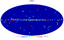
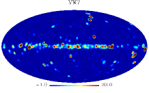
Figure 1: The $K(R)$ (left) and $\bar{K}(R)$ (right) maps for VW7 data. In both maps, we have adopted $R=2^{\circ}$.

It is important to mention that these definitions cannot well localize the non-Gaussian sources. For example, in Fig. 1 the kurtosis map $K(R)$ (left panel), we find the clear circular morphology around the point sources. This means that the values of $K_{j}$ always maximize/minimize at the edge of the circles, rather than the center of the circles. To overcome it and localize the non-Gaussian sources, it is better to define the following average quantities,

$$\bar{X_{j}}(R)=\frac{1}{N_{\rm p}}\sum_{j=1}^{N_{\rm p}}X_{j}(R),$$ (2)

where $X=M,V,S,K$ for mean temperature, standard deviation, skewness and kurtosis. $X_{j}$ is the corresponding local quantities defined above, and $N_{\rm p}$ is again the number of pixels in the $j^{\rm th}$ cap. For the comparison, we plot the corresponding $\bar{K}(R)$ in the right panel of Fig. 1.

Now, let us apply the method to the CMB maps. Firstly, we consider the VW7 map. By choosing $R=2^{\circ}$, we plot $\bar{X}(R)$ maps in Fig. 2. The figures clearly show that these local statistics are sensitive to the foreground residuals and various point sources. From $\bar{M}$-map, one finds that most non-Gaussianities come from the Galactic plane around $b=0^{\circ}$. However, from $\bar{V}$-, $\bar{S}$- and $\bar{K}$-maps, various extra point sources far from the Galactic plane are clearly presented. These contaminations can be well excluded by the KQ75y7 mask (Gold et al., 2011), which is clearly shown in Fig. 3. In this figure, we plot the same figures as those in Fig. 2, but the mask is applied.

Similarly, we also apply the method to ILC7 and NILC5 maps by choosing $R=2^{\circ}$. The results are shown in Fig. 4 and Fig. 5. We find that these ILC maps are much cleaner than VW7 map in all the four $\bar{M}$-, $\bar{V}$-, $\bar{S}$-, $\bar{K}$-maps. Even so, from the $\bar{V}$-, $\bar{S}$-, $\bar{K}$-maps, we also find some non-Gaussian sources in the Galactic plane. In addition, two significant sources at ($l=209.5^{\circ},b=-20.1^{\circ}$) and ($l=184.9^{\circ},b=-5.98^{\circ}$) are clearly presented in ILC7 maps, which have been identified as the known point sources, and excluded by the KQ75y7 mask. NILC5 map is slightly clearer than ILC7, especially the significant point sources at ($l=209.5^{\circ},b=-20.1^{\circ}$) and ($l=184.9^{\circ},b=-5.98^{\circ}$) disappear now. But the contaminations in the Galactic plane are still quite significant.

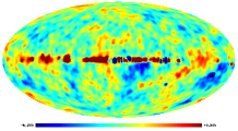
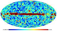
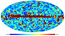
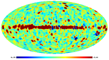
Figure 2: Clockwise, $\bar{M}(R)$ map, $\bar{V}(R)$ map, $\bar{S}(R)$ map and $\bar{K}(R)$ map for VW7, where $R=2^{\circ}$. Note that the $\bar{M}(R)$ and $\bar{V}(R)$ maps have the unit: mK.

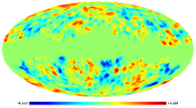
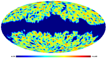
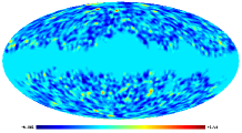
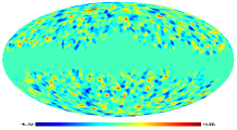
Figure 3: Same as Fig. 2, but KQ75y7 mask has been applied.

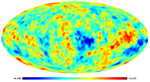
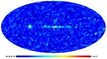
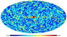
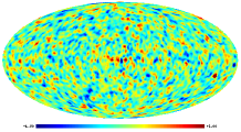
Figure 4: Same as Fig. 2, but VW7 map is replaced by ILC7 map.

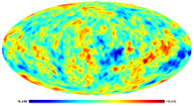
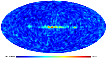
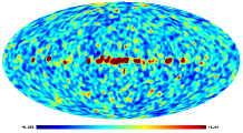
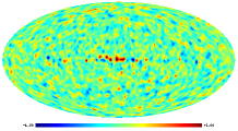
Figure 5: Same as Fig. 2, but VW7 map is replaced by NILC5 map.

3.2 The local properties of WMAP Cold Spot

In this subsection, we shall focus on the local statistics for WMAP CS, and compare with those of the coldest spot in random Gaussian simulations. For a given $\bar{X}(R)$ map ($R=M,V,S$ or $K$) derived from WMAP data, the values of $\bar{X}(R)$ centered at CS are calculated for the scales of $R=1^{\circ}$, $2^{\circ}$, $3^{\circ}$, $4^{\circ}$, $5^{\circ}$, $6^{\circ}$, $7^{\circ}$, $8^{\circ}$, $9^{\circ}$, $10^{\circ}$, $11^{\circ}$, $12^{\circ}$, $13^{\circ}$, $14^{\circ}$, $15^{\circ}$. From Fig. 2, we find in the maps derived from VW7 data, there are many point sources. So, for a fair comparison, in this subsection we shall only consider the ILC7 and NILC5 maps. The statistics for the ILC7 maps are displayed in Fig. 6. We compare them with 500 Gaussian simulations.

For each simulated temperature anisotropy map $\Delta T(\hat{n})$ with $N_{\rm side}=512$, we search for the coldest spot and its position $(l_{c},b_{c})$, which will be used for the comparison. By the exactly same process, we derive the corresponding $\bar{X}(R)$ maps. Then, for each $X$ and $R$, we study the distribution of 500 $\bar{X}_{c}(R)$ values ($\bar{X}_{c}(R)$ is the statistic of the coldest spot in the corresponding simulation), and construct the confident intervals for the statistic. The $68\%$ and $95\%$ confident intervals are illustrated in Fig. 6.

As we can imagine, if CS is simply cold without any other non-Gaussianity, the statistics for $\bar{V}$, $\bar{S}$ and $\bar{K}$ should be normal, i.e. close to the mean values of Gaussian simulations for any $R$. On the other hand, if CS is a combination of some small-scale non-Gaussian structures, as some explanations in (Cruz et al., 2006), the local variance, skewness and kurtosis in small scales should be quite large. However, as we will show below, none of these is the case of WMAP CS.

From Fig. 6, we find that for $\bar{M}$ statistic, WMAP CS is excellently consistent with Gaussian simulations when $R\leq 5^{\circ}$. However, when $R>10^{\circ}$, it deviates from simulations at more than $95\%$ confident level. This is caused by the fact that WMAP CS is surrounded by an anomalous hot ring-like structure, which is firstly noticed by Zhang & Hunterer in (Zhang & Huterer, 2010). For $\bar{V}$ statistic, deviations from Gaussianity outside the $95\%$ confident regions are at the scales $R<2^{\circ}$ and $R>6^{\circ}$. Furthermore, the deviations outside the $95\%$ confident regions are detected in skewness at scales of $R<5^{\circ}$ and in kurtosis at scales of $4^{\circ}<R<7^{\circ}$. For the NILC5 map, the similar deviations for these statistics have also been derived.

Combining these results, we find that WMAP CS seems to be a nontrivial large-scale structure, rather than a combination of some small non-Gaussian structures (for instance, the point sources or foreground residuals, which always follow the non-Gaussianity in the small scales as shown in Fig. 2). This is one of the main conclusions of this paper.

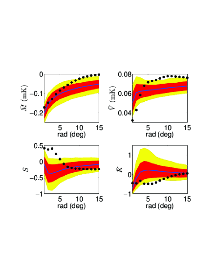
Figure 6: Four statistics for the coldest spots. Confidence regions obtained from 500 Monte Carlo simulations are shown for 68 per cent (dark central region, red online) and 95 per cent (light outer region, yellow online) levels, as is the mean (solid blue line). The observed statistics for WMAP ILC7 map are shown by the solid dots (black online).

We now consider, in more details, the most significant deviation from Gaussianity obtained in Fig. 6. Similar to (McEwen et al., 2005), for each panel of Fig. 6, we define the $\chi^{2}$ statistic as follows:

$$\chi^{2}_{Y}=\sum_{R_{i},R_{j}}(Y_{0}(R_{i})-\overline{Y}(R_{i}))\Sigma^{-1}_{ij}(Y_{0}(R_{j})-\overline{Y}(R_{j})),$$ (3)

where $Y=\bar{M},\bar{V},\bar{S},\bar{K}$. $R_{i}$ and $R_{j}$ run through $1^{\circ}$ to $15^{\circ}$. $Y_{0}(R_{i})$ are the values of the statistics for WMAP CS, and $Y(R_{i})$ are those for the simulations. $\overline{Y}(R_{i})$ is average value of $Y(R_{i})$. $\Sigma$ is the covariance matrix of the vector $Y(R_{i})$. Note that the correlations between $\bar{M}(R_{i})$ and $\bar{M}(R_{j})$ ($i\neq j$) are very strong (the corresponding correlation coefficienta are all larger than 0.6), which significantly affect the corresponding $\chi^{2}_{\bar{M}}$ value, especially when the values of $Y_{0}(R_{i})-\overline{Y}(R_{i})$ oscillate for different $R_{i}$. The total value can also be defined as $\chi^{2}_{tot}=\chi^{2}_{\bar{M}}+\chi^{2}_{\bar{V}}+\chi^{2}_{\bar{S}}+\chi^{2}_{\bar{K}}$. We list the $\chi^{2}_{Y}$ values (Case 1) in Table 1 for ILC7 and in Table 2 for NILC5. In order to be compared with Gaussian simulations, for each realization, we repeat the calculation in Eq.(3), but the quantities $Y_{0}(R_{i})$ of WMAP CS are replaced by the corresponding quantities of the Gaussian realization. Fig. 7 illustrates the histogram of $\chi^{2}_{tot}$ statistic for the ILC7 based map, where we find that WMAP CS in ILC7 deviates from Gaussianity at the $99.0\%$ significant level. At the same time, we also obtain the same results from NILC5 map.

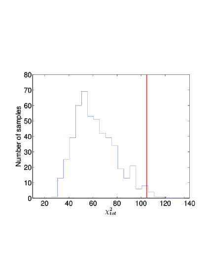
Figure 7: Histogram of the $\chi^{2}_{tot}$ statistic for the coldest spots obtained from 500 Monte Carlo simulations. The observed statistic for WMAP ILC7 map is shown by the solid vertical line (red online).

Table 1: The $\chi^{2}$ values of various statistics for ILC7 based maps. In Case 1, WMAP CS compares with the coldest spots in 500 random Gaussian simulations, in Case 2, WMAP CS compares with the spots at ($l=209^{\circ}$,$b=-57^{\circ}$) in 500 simulations, and Case 3 is same with Case 2, but a cosmic texture has been superimposed in each simulated sample.

	$\chi^{2}_{\bar{M}}$	$\chi^{2}_{\bar{V}}$	$\chi^{2}_{\bar{S}}$	$\chi^{2}_{\bar{K}}$	$\chi^{2}_{tot}$
Case 1	32.95	34.95	24.13	12.64	104.66
Case 2	35.16	43.27	31.83	10.46	120.73
Case 3	34.01	29.04	12.76	7.40	83.21

Table 2: Same as Table 1, but for NILC5 maps.

	$\chi^{2}_{\bar{M}}$	$\chi^{2}_{\bar{V}}$	$\chi^{2}_{\bar{S}}$	$\chi^{2}_{\bar{K}}$	$\chi^{2}_{tot}$
Case 1	31.59	26.27	35.42	11.73	105.02
Case 2	33.67	36.23	43.24	13.54	126.68
Case 3	31.17	25.27	19.82	11.03	87.29

3.3 Compared with simulations including cosmic texture

In (Cruz et al., 2007b, 2008), by studying the temperature and area of CS, the authors found that the cosmic texture, rather than the other explanations, provided an excellent interpretation for the WMAP CS. In this subsection, we shall study whether the local anomalies of CS found in this work are consistent with the cosmic texture explanation.

We firstly study how the WMAP CS deviates from the normal spot of the CMB map. We compare the CS with the spots at $(l=209^{\circ},b=-57^{\circ})$ in the Gaussian random simulations. The statistics are displayed in Fig. 8, with the confidence intervals constructed from the Monte Carlo simulations. As anticipated, we find that the CS is colder than simulations in the small scales. Especially, when $R\leq 4^{\circ}$, it deviates from simulations at more than $95\%$ confident level. However, as $R$ increases, the deviation becomes smaller and smaller. Furthermore, we find that for the $\bar{V}$ and $\bar{S}$ statistics, WMAP CS deviates from simulations at larger scales, i.e. it deviates at more than $95\%$ confident level when $R>4^{\circ}$ for the $\bar{V}$ statistic and when $R>12^{\circ}$ for the $\bar{S}$ statistic. The similar results are also obtained from NILC5 map and the masked VW7 map (see Fig. 9).

The $\chi^{2}$ statistic defined in Eq.(3) is also applied here. In Tables 1, 2 and 3 (Case 2), we list the values of $\chi_{Y}^{2}$ and $\chi_{tot}^{2}$ for ILC7, NILC5 and masked VW7, respectively. Compared with the Gaussian simulations, ILC7 CS deviates from Gaussianity at the $99.0\%$ significant level (see Fig. 10), NILC5 CS deviates at the $89.8\%$ significant level, and the masked VW7 CS deviates at the $99.4\%$ significant level (see Fig. 11).

Now, let us study the cosmic texture interpretation. The profile for the CMB temperature fluctuation caused by a collapsing cosmic texture is given by

$$\frac{\Delta T}{T}=-\left\{\begin{array}[]{ll}\frac{\varepsilon}{\sqrt{1+4\left(\frac{\vartheta}{\vartheta_{c}}\right)^{2}}}&\mathrm{if}~{}~{}\vartheta\leq\vartheta_{*}\\ &\\ \frac{\varepsilon}{2}\mathrm{e}^{-\frac{1}{2\vartheta^{2}_{c}}\left(\vartheta^{2}+\vartheta^{2}_{*}\right)}&\mathrm{if}~{}~{}\vartheta>\vartheta_{*}\\ \end{array}\right.,$$ (4)

where $\vartheta$ is the angle from the center. $\varepsilon$ is the amplitude parameter, and $\vartheta_{c}$ is the scale parameter. $\vartheta_{*}=\sqrt{3}/2\vartheta_{c}$. By the Bayesian analysis, the texture parameters were obtained $\varepsilon=7.3^{+2.5}_{-3.6}\times 10^{-5}$ and $\vartheta_{c}=4.9^{+2.8}_{-2.4}{\rm deg}$ at $95\%$ confidence (Cruz et al., 2007b).

In our calculation, we adopt the best-fit texture parameters $\varepsilon=7.3\times 10^{-5}$ and $\vartheta_{c}=4.9^{\circ}$. Now, in order to taking the cosmic texture into account, for each realization we superimpose the texture morphology at the same position $(l=209^{\circ},b=-57^{\circ})$, and repeat the exactly same analyses. The results are also shown in Figs. 12-15. Interestingly enough, we find that WMAP CS is exactly consistent with the simulations if the cosmic texture is considered. For each statistic, the value of WMAP CS is equal to the mean value of simulations in nearly 1-$\sigma$ confident level.

From Tables 1-3, we find that once the cosmic texture is considered in simulations, compared with the pure Gaussian samples, every $\chi^{2}_{Y}$ value reduces, especially for $Y=\bar{V}$ and $Y=\bar{S}$. Note that the $\chi^{2}_{Y}$ value for $Y=\bar{M}$ has no significantly reduction, which is caused by the following two facts: First, the cross-correlations between $\bar{M}(R_{i})$ and $\bar{M}(R_{j})$ ($i\neq j$) are very strong; Second, the values of $Y_{0}(R_{i})-\bar{Y}(R_{i})$ oscillate for different $R_{i}$. For the $\chi_{tot}^{2}$ statistic of ILC7 CS, the significant level of the deviation from simulations reduces to $90.0\%$, and that of VW7 CS becomes $87.4\%$. So, we conclude that the cosmic texture can excellently account for the excesses of $\bar{M}$, $\bar{V}$ and $\bar{S}$ of WMAP CS, and the local analyses of WMAP CS strongly support the cosmic texture explanation.

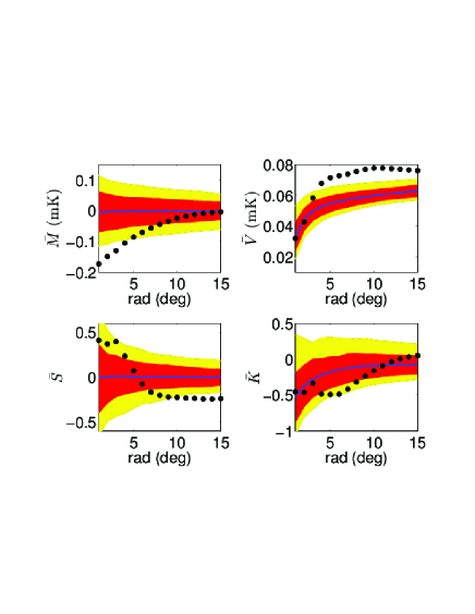
Figure 8: Four statistics for the spot at $(l=209^{\circ},b=-57^{\circ})$. Confidence regions obtained from 500 Monte Carlo simulations are shown for 68 per cent (dark central region, red online) and 95 per cent (light outer region, yellow online) levels, as is the mean (solid blue line). The observed statistics for WMAP ILC7 map are shown by the solid dots (black online).

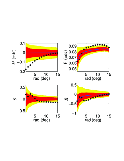
Figure 9: Same as Fig. 8, but ILC7 map is replaced by the masked VW7 maps.

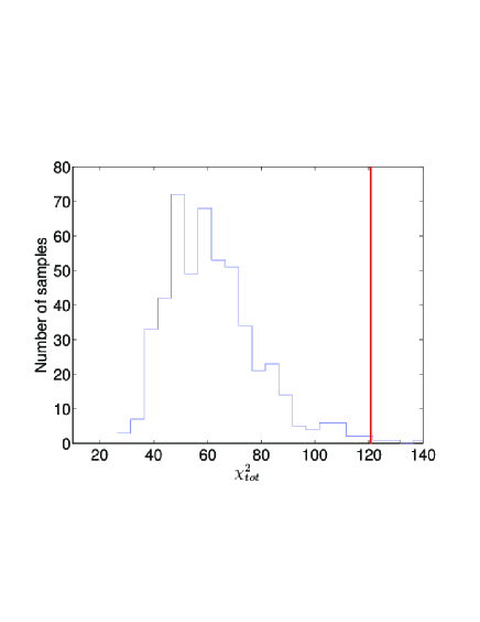
Figure 10: Histograms of the $\chi^{2}_{tot}$ statistic for the spots at $(l=209^{\circ},b=-57^{\circ})$ obtained from 500 Monte Carlo simulations. The observed statistic for WMAP ILC7 map is shown by the solid vertical line (red online).

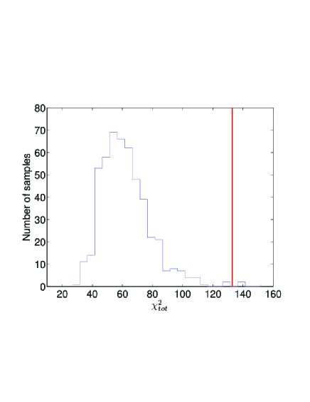
Figure 11: Same as Fig. 10, but ILC7 map is replaced by the masked VW7 maps.

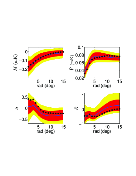
Figure 12: Four statistics for the spot at $(l=209^{\circ},b=-57^{\circ})$. Confidence regions obtained from 500 Monte Carlo simulations are shown for 68 per cent (dark central region, red online) and 95 per cent (light outer region, yellow online) levels, as is the mean (solid blue line). Note that the cosmic texture is superimposed in each simulation. The observed statistics for WMAP ILC7 map are shown by the solid dots (black online).

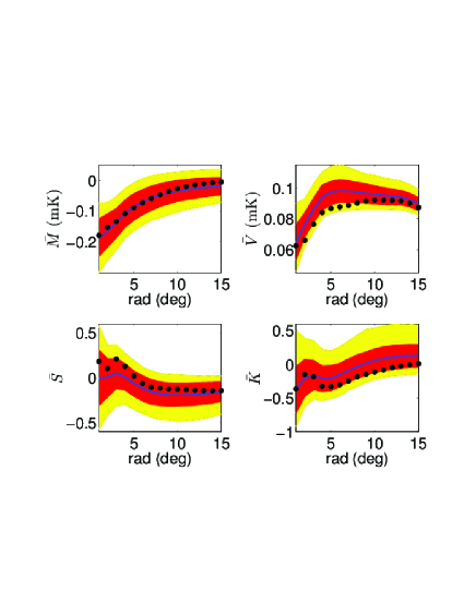
Figure 13: Same as Fig. 12, but ILC7 map is replaced by the masked VW7 maps.

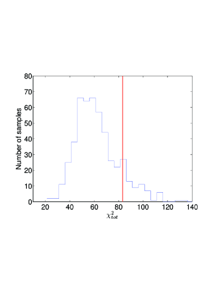
Figure 14: Histograms of the $\chi^{2}_{tot}$ statistic for the spots at $(l=209^{\circ},b=-57^{\circ})$ obtained from 500 Monte Carlo simulations. Note that the cosmic texture is superimposed in each simulation. The observed statistic for WMAP ILC7 map is shown by the solid vertical line (red online).

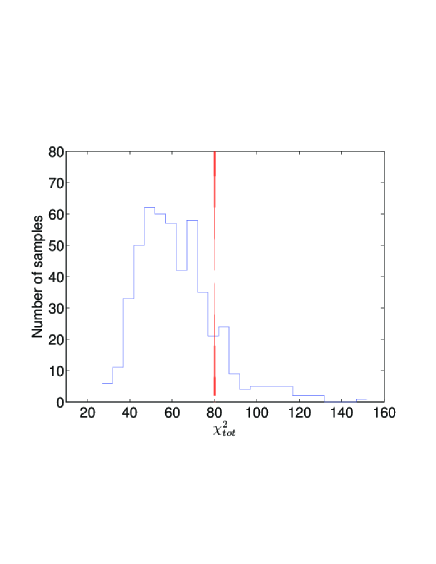
Figure 15: Same as Fig. 14, but ILC7 map is replaced by the masked VW7 maps.

Table 3: Same as Table 1, but for the masked VW7 maps in Case 2 and Case 3.

	$\chi^{2}_{\bar{M}}$	$\chi^{2}_{\bar{V}}$	$\chi^{2}_{\bar{S}}$	$\chi^{2}_{\bar{K}}$	$\chi^{2}_{tot}$
Case 2	32.67	38.40	46.00	15.90	132.97
Case 3	16.12	22.97	30.53	10.52	80.14

4 Cold spot and WMAP low multipoles

If WMAP CS is a large-scale non-Gaussian structure, as we have found in previous section, the non-Gaussianity caused by CS should be encoded in the low multipoles, rather than the high multipoles. In this section, we shall confirm it by studying the effect of different multipoles on the WMAP non-Gaussian signals.

Following (Vielva et al., 2004; Cruz et al., 2005, 2006; Zhang & Huterer, 2010), in this section we study the non-Gaussianity of WMAP data by using the wavelet transform, which can emphasize or amplify some features of the CMB data at a particular scale. The SMHWs are defined as

$$\Psi(\theta;R)=A(R)(1+(\frac{y}{2})^{2})^{2}(2-(\frac{y}{2})^{2})e^{{-y^{2}}/{2R^{2}}},$$ (5)

where $y\equiv 2\tan(\theta/2)$ is the stereographic projection variable, and $\theta\in[0,\pi)$ is the co-latitude. $R$ is the scale, and $A$ is the constant for the normalization, which can be written as

$$A(R)=\left[2\pi R^{2}\left(1+\frac{R^{2}}{2}+\frac{R^{4}}{4}\right)\right]^{-1/2}.$$ (6)

The continuous wavelet transform stereographically projected over the sphere with respect to $\Psi(\theta;R)$ is given by

$$T_{\rm w}({\hat{r}};R)=\int d\Omega^{\prime}T({\hat{r}+\hat{r}^{\prime}})\Psi(\theta^{\prime};R),$$ (7)

where ${\hat{r}}=(\theta,\phi)$ and ${\hat{r}^{\prime}}=(\theta^{\prime},\phi^{\prime})$ are the stereographic projections to sphere of center of the spot and the dummy location, respectively. In our analyses of this section, the locations of centroids of spots are chosen to be centers of pixels in $N_{\rm side}=32$ resolution. Following (Zhang & Huterer, 2010), we define the occupancy fraction as follows to account for the masked parts of the sky,

$$N_{\rm w}({\hat{r}};R)=\int d\Omega^{\prime}M({\hat{r}+\hat{r}^{\prime}})\Psi^{2}(\theta^{\prime};R),$$ (8)

where $M(\hat{r})$ is KQ75y7 mask (Gold et al., 2011). In order to reduce the biases due to masking, we only include the results of for which $N_{\rm w}({\hat{r}};R)>0.95$.

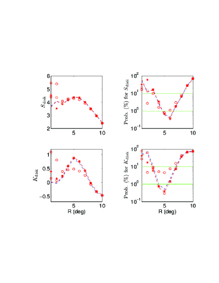
Figure 16: Values and probabilities of the statistics $S_{\rm disk}$ (upper) and $K_{\rm disk}$ (lower) for various cases. In each panel, the dark line (blue online) is for the results of VW7 map, and grey line (red online) is for ILC7 map. The circles (red online) are for the ILC7 with $l_{\max}=20$, the crosses (red online) are for that with $l_{\max}=40$, and the squares (red online) are for that with $l_{\max}=100$.

In our analyses of this section, we shall consider the VW7 and ILC7 data. We degrade them to a lower resolution $N_{\rm side}=128$, then apply the KQ75y7 mask. For each masked WMAP data, we use the SMHW transform in Eq. (7) to get the corresponding map in wavelet domain $T_{\rm w}({\hat{r}};R)$. To investigate the non-Gaussianity in different scales, for each map we consider the cases with $R=1^{\circ}$, $2^{\circ}$, $3^{\circ}$, $4^{\circ}$, $5^{\circ}$, $6^{\circ}$, $7^{\circ}$, $8^{\circ}$, $9^{\circ}$, $10^{\circ}$. Similar to many authors (Vielva et al., 2004; Cruz et al., 2005, 2006; Zhang & Huterer, 2010), we define the statistics $S_{\rm disk}$ and $K_{\rm disk}$ as follows to study the non-Gaussianity related to WMAP CS:

$$S_{\rm disk}(R) = \frac{T_{\rm w}^{\rm coldest}(\hat{r};R)}{\sigma_{\rm w}(R)},$$ (9)

$$K_{\rm disk}(R) = \frac{1}{N_{\rm spots}}\frac{\sum_{i=1}^{N_{\rm spots}}T^{4}_{\rm w}(\hat{r}_{i};R)}{\sigma^{4}_{\rm w}(R)}-3.$$ (10)

Here $\sigma_{\rm w}(R)$ is the standard deviation of the distribution of all spots in a given map, and $T_{\rm w}^{\rm coldest}(\hat{r},R)$ is the coldest spot in this distribution. From the definitions, we find that $S_{\rm disk}(R)$ describes the cold spot significance, and $K_{\rm disk}(R)$ is the kurtosis of spots in a given map. In Fig. 16 (left panels), we present the values of $S_{\rm disk}(R)$ and $K_{\rm disk}(R)$ for different scale parameter $R$. Both VW7 and ILC7 illustrate the same results: the values of both $S_{\rm disk}(R)$ and $K_{\rm disk}(R)$ maximize at $R\sim 5^{\circ}$. The results then are compared with 2000 randomly generated Gaussian simulations, with the exactly same methodology applied. So we can get the probabilities of simulations, which have the larger $S_{\rm disk}(R)$ or $K_{\rm disk}(R)$ than those of WMAP data. These probabilities for both statistics are also shown in Fig. 16 (right panel). So, similar to other works (Vielva et al., 2004; Cruz et al., 2005; Zhang & Huterer, 2010), we find that when $R=4^{\circ}-6^{\circ}$, WMAP data have the deviations from the Gaussian simulations, i.e. the corresponding probabilities for the statistics $S_{\rm disk}(R)$ and/or $K_{\rm disk}(R)$ are smaller than $1\%$.

Now, let us study which multipoles account for the non-Gaussianity above. We consider the original ILC7 map $T(\hat{r})$, and expand it via spherical harmonic composition:

$$T(\hat{r})=\sum_{l,m}a_{lm}Y_{lm}(\hat{r}),$$ (11)

where $Y_{lm}$ are the spherical harmonics and $a_{lm}$ are the corresponding coefficients. Then the new map can be constructed as follows:

$$T^{\prime}(\hat{r})=\sum_{l=2}^{l_{\max}}\sum_{m=-l}^{l}a_{lm}Y_{lm}(\hat{r}).$$ (12)

It is clear that this new map includes only the low multipoles $l\in[2,~{}l_{\max}]$. Thus, we can repeat the processes above, but the ILC7 map $T(\hat{r})$ is replaced by $T^{\prime}(\hat{r})$. In the analyses, we choose three cases with $l_{\max}=20$, $l_{\max}=40$ and $l_{\max}=100$ to study the effect of different multipoles, and show the results in Fig. 16 with circles, crosses and squares, respectively. We find that for the statistic $S_{\rm disk}(R)$, if the lowest multipoles $l\leq 20$ are considered, the values of the statistic and the corresponding probabilities are quite close to those gotten in the map including all the multipoles. These clearly show that the coldness of CS are mainly encoded in these lowest multopole range, which is consistent with the conclusion in (Naselsky et al., 2010). While for the statistic $K_{\rm disk}(R)$, we find the WMAP data are quite normal for the case with $l_{\max}=20$, compared with the Gaussian simulations. However, if $l_{\max}=40$ is considered, the results for both statistics are very close to those in the map with all multipoles. So we conclude that WMAP CS reflects directly the peculiarities of the low multipoles $l\leq 40$, which suggests that CS should be a large-scale non-Gaussian structure, rather than a combination of some small structures. This consists with our conclusion in Section 3.

5 Conclusions

Since the discovery of the non-Gaussian Cold Spot in WMAP data, it has attracted a great deal of attention, and many explanations have been proposed. To distinguish them, in this paper we have studied the local properties of WMAP CS at different scales by introducing the local statistics including the mean temperature, variance, skewness and kurtosis. Compared with the coldest spots in random Gaussian simulations, WMAP CS deviates from Gaussianity at $\sim 99\%$ significant level, and the non-Gaussianity of CS exists at all the scales $1^{\circ}<R<15^{\circ}$. However, when compared with the spots at the same position in the simulated Gaussian maps, we found the significant excesses of local variance and skewness in the large scales $R>5^{\circ}$, rather than in the small scales. Furthermore, we found that the non-Gaussianity caused by CS is totally encoded in the WMAP low multipoles $l\leq 40$. These all imply that WMAP CS is a large-scale non-Gaussian structure, rather than the combination of some small structures.

It was claimed by many authors that the cosmic texture with a characteristic scale about $10^{\circ}$, rather than other mechanisms, could provide the excellent explanation for WMAP CS. By comparing with the random simulations including the similar texture structure, we found this non-Gaussian structure could excellently explain the excesses of the statistics. So our results in this paper strongly support the cosmic texture explanation.

In the end of this paper, it is important to mention that the non-Gaussianity of WMAP CS has been confirmed by the new Planck observations (Planck Collaboration, 2013) on the CMB temperature. In the near future, the polarization results of Planck mission will be released, which would play a crucial role to test the WMAP CS, as well as to reveal its physical origin (Cruz et al., 2007b).

References

- Basak & Delabrouille (2012) Basak S. & Delabrouille J. 2012, MNRAS, 419, 1163
- Bennett et al. (2003) Bennett C. L. et al., 2003, ApJS, 148, 1
- Bennett et al. (2011) Bennett C. L. et al., 2011, ApJS, 192, 17
- Bernui & Reboucas (2009) Bernui A. & Reboucas M. J. 2009, PRD, 79, 063528
- Bernui & Reboucas (2010) Bernui A. & Reboucas M. J. 2010, PRD, 81, 063533
- Bernui & Reboucas (2012) Bernui A. & Reboucas M. J. 2012, PRD, 85, 023522
- Bremer et al. (2010) Bremer M. N., Silk J., Davies L. J. M. & Lehnert M. D. 2010, MNRAS, 404, L69
- Cayon et al. (2005) Cayon L., Lin J. & Treaster A. 2005, MNRAS, 362, 826
- Cruz et al. (2005) Cruz M., Martinez-Gonzalez E., Vielva P. & Cayon L. 2005, MNRAS, 356, 29
- Cruz et al. (2006) Cruz M., Tucci M., Martinez-Gonzalez E. & Vielva P. 2006, MNRAS, 369, 57
- Cruz et al. (2007a) Cruz M., Cayon L., Martinez-Gonzalez E. & Vielva P. 2007, ApJ, 655, 11
- Cruz et al. (2007b) Cruz M., Turok N., Vielva P., Martinez-Gonzalez E. & Hobson M. P. 2007, Science, 318, 1612
- Cruz et al. (2008) Cruz M., Martinez-Gonzalez E., Vielva P., Diego J. M., Hobson M. & Turok N. 2008, MNRAS, 390, 913
- Delabrouille et al. (2009) Delabrouille J., Cardoso J. F., Le Jeune M., Betoule M., Fay G. & Guilloux F. 2009, A&A, 493, 835
- Doroshkevich et al. (2005) Doroshkevich A. G., Naselsky P. D., Verkhodanov O. V., Novikov D. I., Turchaninov V. I., Novikov I. D., Christensen P. R. & Chiang L. -Y. 2005, International Journal of Modern Physics D, 14, 275
- Gold et al. (2011) Gold B. et al., 2011, ApJS, 192, 15
- Gorski et al. (2005) Gorski K. M., Hivon E., Banday A. J., Wandelt B. D., Hansen F. K., Reinecke M. & Bartelman M. 2005, ApJ, 622, 759
- Granett et al. (2009) Granett B. R., Szapudi I. & Neyrinck M. C. 2009, ApJ, 714, 825
- Hansen et al. (2012) Hansen M., Zhao W., Frejsel A. M., Naselsky P. D., Kim J. & Verkhodanov O. V. 2012, MNRAS, 426, 57
- Hinshaw et al. (2007) Hinshaw G. et al., 2007, ApJS, 170, 288
- Inoue & Silk (2006) Inoue K. T. & Silk J. 2006, ApJ, 648, 23
- Inoue & Silk (2007) Inoue K. T. & Silk J. 2006, ApJ, 664, 650
- Inoue (2012) Inoue K. T. 2012, MNRAS, 421, 2731
- Komatsu et al. (2011) Komatsu E. et al., 2011, ApJS, 192, 18
- McEwen et al. (2005) McEwen J. D., Hobson M. P., Lasenby A. N. & Mortlock D. J. 2005, MNRAS, 359, 1583
- Naselsky et al. (2010) Naselsky P. D., Christensen P. R., Coles P., Verkhodanov O., Novikov D. & Kim J. 2010, Astrophys. Bull., 65, 101
- Planck Collaboration (2013) Planck Coolaboration, arXiv:1303.5083
- Rudnick et al. (2007) Rudnick L., Brown, S. & Williams L. R. 2007, ApJ, 671 40
- Smith & Huterer (2010) Smith K. M. & Huterer D. 2010, MNRAS, 403, 2
- Vielva et al. (2004) Vielva P., Martinez-Gonzalez E., Barreiro R. B., Sanz J. L. & Cayon L. 2004, ApJ, 609, 22
- Vielva (2010) Vielva P. 2010, arXiv:1008.3051
- Zhang & Huterer (2010) Zhang R. & Huterer D. 2010, Astroparticle Physics, 33, 69