Geometric properties of Kahan’s method

Abstract

We show that Kahan’s discretization of quadratic vector fields is equivalent to a Runge–Kutta method. When the vector field is Hamiltonian on either a symplectic vector space or a Poisson vector space with constant Poisson structure, the map determined by this discretization has a conserved modified Hamiltonian and an invariant measure, a combination previously unknown amongst Runge–Kutta methods applied to nonlinear vector fields. This produces large classes of integrable rational mappings in two and three dimensions, explaining some of the integrable cases that were previously known.

1 Introduction: Kahan’s method for quadratic vector fields

Consider a system of differential equations arising from a quadratic vector field

$$\dot{x}=f(x):=Q(x)+Bx+c,\quad x\in\mathbb{R}^{n},$$ (1)

where $Q$ is an $\mathbb{R}^{n}$-valued quadratic form, $B\in\mathbb{R}^{n\times n}$, and $c\in\mathbb{R}^{n}$. Consider the numerical integration method $x\mapsto x^{\prime}$ with step size $h$ given by

$$\frac{x^{\prime}-x}{h}=Q(x,x^{\prime})+\frac{1}{2}B(x+x^{\prime})+c$$ (2)

where

$$Q(x,x^{\prime})=\frac{1}{2}\left(Q(x+x^{\prime})-Q(x)-Q(x^{\prime})\right)$$ (3)

is the symmetric bilinear form obtained from the quadratic form $Q$ by polarisation. We call (2) the Kahan method. It is symmetric (i.e., self-adjoint), and, crucially, it is only linearly implicit, that is, $x^{\prime}$ can be computed by solving a single linear system (because the right hand side of (2) is linear in $x^{\prime}$). The method (2) was introduced by Kahan in [8] for two examples, a scalar Riccati equation and a 2-dimensional Lotka–Volterra system ([8], p. 14) and written down in the general form (2) in [9] (see also references therein).

Because of the different treatment of each term and the unusual treatment of the quadratic term, Kahan called (2) an ‘unconventional’ method.

The map obtained from applying the Kahan method to various quadratic vector fields $f$ has been shown to be completely integrable in a number of cases (see [5], [6], [10], and references therein). In most cases, the conserved quantities depend on the step size $h$. At present there is no single ‘integrability mechanism’ known which accounts for all integrable cases.

In this paper we show that the Kahan method is a Runge–Kutta method. As such it shares a number of features with all Runge–Kutta methods: it has a B-series, it is affine covariant, and it preserves all affine symmetries and all linear integrals of $f$ automatically. As a symmetric linear method it preserves all affine reversing symmetries of $f$ automatically, and the B-series of its modified vector field contains only even powers of $h$.

We then consider the case that $f$ is a Hamiltonian vector field on either a symplectic vector space or a Poisson vector space with constant Poisson structure, in any dimension $n$. We show that in this case the Kahan map has a conserved quantity that converges to the Hamiltonian of the vector field as $h\to 0$. It also has a conserved measure which converges to the Euclidean measure as $h\to 0$. These general properties explain some of the integrable cases considered in [10].

2 Kahan’s method as a Runge–Kutta method

Proposition 1.

The Kahan method coincides with the Runge–Kutta method

$$\frac{x^{\prime}-x}{h}=-\frac{1}{2}f(x)+2f\Big{(}\frac{x+x^{\prime}}{2}\Big{)}-\frac{1}{2}f(x^{\prime})$$ (4)

restricted to quadratic vector fields.

Proof.

We have

 

$${\frac{x^{\prime}-x}{h}}$$

  (5)

∎

(Many other Runge–Kutta methods also coincide with the Kahan method when restricted to quadratic vector fields. In this paper, we restrict our attention to (4).) As already noted by Kahan [9], the Kahan method also coincides with a certain Rosenbrock method on quadratic vector fields, for expanding in Taylor series about $x$ gives

 

$${\frac{x^{\prime}-x}{h}}$$

  (6)

so

$$\frac{x^{\prime}-x}{h}=\Big{(}I-\frac{h}{2}f^{\prime}(x)\Big{)}^{-1}f(x).$$ (7)

From the symmetry of the method, or by expanding instead around $x^{\prime}$, Kahan’s method can also be written

$$\frac{x^{\prime}-x}{h}=\Big{(}I+\frac{h}{2}f^{\prime}(x^{\prime})\Big{)}^{-1}f(x^{\prime}).$$ (8)

The B-series of this method is

$$x^{\prime}=x+\sum_{k=0}^{\infty}\frac{h^{k+1}}{2^{k}}f^{\prime}(x)^{k}f(x),$$

that is, it contains only tall trees. (For nonquadratic vector fields, the methods (7) and (4) are not necessarily equivalent.)

The Runge–Kutta method (4) has 3 stages and Butcher tableau

0	0	0	0
$\frac{1}{2}$	$-\frac{1}{4}$	1	$-\frac{1}{4}$
1	$-\frac{1}{2}$	2	$-\frac{1}{2}$
	$-\frac{1}{2}$	2	$-\frac{1}{2}$

The modified vector field of the Kahan method applied to quadratic vector fields can be calculated using standard methods [4]. Its first few terms are

 

$${f+}$$

 

A calculation using conjugation by B-series, considering only quadratic vector fields, now yields the following result. We omit the details.

Proposition 2.

Kahan’s method applied to general quadratic fields has order 2 and is conjugate to symplectic up to order 4. It is not conjugate by B-series to a method of order greater than 2 or conjugate-symplectic by B-series to order higher than 4.

3 Conservative properties of Kahan’s method

We now consider the conservative properties of the Kahan method in the case of canonical Hamiltonian systems $\dot{x}=J^{-1}\nabla H(x)$ where $H:\mathbb{R}^{n}\to\mathbb{R}$ is the Hamiltonian or energy of the system. First, note that the method (4) is the $a=-1/2$ member of the class of Runge–Kutta methods

$$\frac{x^{\prime}-x}{h}=af(x)+(1-2a)f\Big{(}\frac{x+x^{\prime}}{2}\Big{)}+af(x^{\prime}).$$ (9)

These are all symmetric, A-stable, and second order. Some other members of this family are also known to have conservative properties:

1. When $a=0$, we have the midpoint rule. It is symplectic for canonical Hamiltonian systems. Because it is symplectic, it conserves the Euclidean measure. When the Hamiltonian $H$ is analytic, the method has a formal invariant $\widetilde{H}=H+\sum_{k=1}^{\infty}h^{k}H_{k}$. When $H$ is quadratic (i.e. when $f$ is linear) this series converges to give a conserved quantity of the method.

2. When $a=1/2$, we have the trapezoidal rule. It is conjugate to the midpoint rule (the conjugacy being half an Euler step), and so it is also conjugate to symplectic and hence conserves a measure close to the Euclidean measure, and it also has a formal invariant close to $H$.

3. When $a=1/6$, we have ‘Simpson’s method’ [2], so-called because the right hand side of (9) is Simpson’s quadrature of $A=\int_{0}^{1}f(\xi x+(1-\xi)x^{\prime})\,d\xi$, appearing in the average vector field method $\frac{x^{\prime}-x}{h}=A$, which conserves the Hamiltonian in canonical Hamiltonian systems. Simpson’s method preserves quartic Hamiltonians exactly because it coincides with the average vector field method in that case. It is not conjugate to symplectic in the sense of B-series [4].

Proposition 3.

Kahan’s method has a conserved quantity given by the modified Hamiltonian

$$\widetilde{H}(x):=H(x)+\frac{1}{3}h\nabla H(x)^{T}\Big{(}I-\frac{1}{2}hf^{\prime}(x)\Big{)}^{-1}f(x)$$ (10)

for all cubic Hamiltonian systems on symplectic vector spaces and on all Poisson vector spaces with constant Poisson structure. The modified Hamiltonian is (i) a rational function of $x$; (ii) an even function of $h$; and (iii) given by a convergent series of elementary Hamiltonians containing only even-order tall trees.

Proof.

We first consider the homogeneous case, i.e., we let $f=K\nabla H(x)$ where $K$ is an arbitrary (not necessarily invertible) constant antisymmetric matrix and $H(x)=C(x,x,x)$ where $C$ is a symmetric trilinear form. Note that $\nabla H(x)^{T}v=3C(x,x,v)$ for all $x$, $v\in\mathbb{R}^{n}$. For any of the methods (9), we have (writing $\bar{x}=(x+x^{\prime})/2$)

 

$${0}$$

 

The case $a=\frac{1}{6}$ is Simpson’s method, confirming that $H(x)$ is conserved in that case.

For Kahan’s method, $a=-\frac{1}{2}$, and we have from Eqs. (7,8) that

 

$${x^{\prime\prime}-x}$$

 

Therefore

 

$${C(x^{\prime},x^{\prime},x^{\prime\prime})-C(x,x,x^{\prime})}$$

  (11)

because each matrix in square brackets is antisymmetric. (Each term is an elementary Hamiltonian corresponding to a superfluous tall tree.) The expression is a rational function of $x$ and $h$ so if its Taylor series in $h$ is zero, the function is zero. Therefore the Kahan method has a first integral $C(x,x,x^{\prime})$. This can also be written in the symmetric form

$$C(x,x,x^{\prime})=(C(x,x,x^{\prime})+C(x,x^{\prime},x^{\prime}))/2=C(x,(x+x^{\prime})/2,x^{\prime})$$

or explicitly as a function of $x$ as

 

$${C(x,x,x^{\prime})}$$

 

As in (11), $\nabla H(x)^{T}f^{\prime}(x)^{2n}f(x)=0$ for all $n$, so we can also write $\widetilde{H}(x)$ in a form manifestly even in $h$,

$$\widetilde{H}(x)=H(x)+\frac{1}{6}h^{2}\nabla H(x)^{T}\Big{(}I-\frac{1}{2}h^{2}f^{\prime}(x)^{2}\Big{)}^{-1}f^{\prime}(x)f(x).$$

Now consider the case that $H(x)$ is cubic but not homogeneous. We extend it to a homogeneous function $\overline{H}(x_{0},x_{1},\dots,x_{n})$ so that $\overline{H}(1,x_{1},\dots,x_{n})=H(x_{1},\dots,x_{n})$, and extend $K$ to $\overline{K}$ by adding a zero initial row and column, so that $\dot{x}_{0}=0$. The linear integral $x_{0}$ is conserved by Kahan’s method, and $\overline{K}\nabla\overline{H}(1,x)=K\nabla H(x)$, so the modified Hamiltonian of Kahan’s method for $\overline{K}\nabla\overline{H}(x)$ reduces to a modified Hamilton of Kahan’s method for $K\nabla H(x)$ given by the same formula (10) as in the homogeneous case. ∎

The Kahan map and its conserved quantity $\widetilde{H}$ are rational functions of $x$ whose degrees are described in the following proposition. When $K$ has full rank, for $n=2$ (resp. $3,4$), $\widetilde{H}$ is degree 3 over degree 2 (resp. degree 5/2, degree 5/4) and the Kahan map is degree 2/2 (resp. degree 3/2, degree 4/4). In the planar case, Kahan’s method gives a rational map with cubic invariant curves. We conjecture that the dynamics of the Kahan map in two dimensions is related to the abelian group structure of elliptic curves (and in higher dimensions, to that of abelian varieties) as is the case for planar QRT maps [3].

Proposition 4.

Let $H$ be a cubic in $\mathbb{R}^{n}$ and let $K$ be a rank $k$ antisymmetric $n\times n$ matrix.

1. The degree of the denominator of $\widetilde{H}$ is at most $k$ and the degree of the numerator of $\widetilde{H}$ is at most $k+3$. When $k=n$ the degree of the numerator of $\widetilde{H}$ is at most $k+1$.

2. The degree of the denominator of the Kahan map is at most $k$ and the degree of the numerator is at most $k+1$. When $k=n$ the degree of the numerator is at most $k$.

Proof.

1. Because the method is linearly covariant we can assume without loss of generality that $K$ is in its Darboux normal form

   $$K=\left(\matrix{L&0\cr 0&0}\right),\quad L=\left(\matrix{0&I\cr-I&0}\right)$$

   where $L$ is $k\times k$. Numbering the blocks of $K$ 1 and 2, the denominator of $\widetilde{H}$ is equal to

    

   $${\det(I-\frac{1}{2}hf^{\prime})}$$

    

   Each entry of the matrix $LH_{11}(x)$ is linear in $x$ so the final determinant has degree at most $k$. Next, we write

   $$\widetilde{H}(x)=\frac{H(x)\det(I-\frac{1}{2}hf^{\prime}(x))+\frac{1}{3}h(\nabla H(x))^{T}\mathop{\rm adj}(I-\frac{1}{2}hf^{\prime}(x))f(x)}{\det(I-\frac{1}{2}hf^{\prime}(x))}$$

   where $\mathop{\rm adj}(A)=A^{-1}\det A$ is the adjoint of $A$. The first term in the numerator has degree at most $k+3$, $\nabla H$ and $f$ have degree at most 2, and $\mathop{\rm adj}(I-\frac{1}{2}hf^{\prime}(x))f(x)=\mathop{\rm adj}(I-\frac{1}{2}hLH_{11}(x))LH_{1}(x)$ where each entry in $\mathop{\rm adj}(I-\frac{1}{2}hf^{\prime}(x))$ is the determinant of a $(k-1)\times(k-1)$ matrix whose entries are linear in $x$. Hence the degree of the numerator of $\widetilde{H}(x)$ is at most $k+3$.

   Finally we consider the case $k=n$. Since $k$ is even, $n$ must be even. First consider the case that $H$ is a homogeneous cubic. Then $\nabla H(x)=\frac{1}{2}H^{\prime\prime}(x)x$ and $H(x)=\frac{1}{6}x^{T}H^{\prime\prime}(x)x$. Thus in this case we have

    

   $${6\widetilde{H}(x)}$$

    

   Expanding the matrix inverse using Cramer’s rule now shows that the degree of the numerator is at most $k+2$. The terms of degree $k+2$ come from terms in the minors of $I-\frac{1}{2}hKH^{\prime\prime}(x)$ of degree $k-1$ in $x$. Every $x_{i}$ in the matrix $I-\frac{1}{2}hKH^{\prime\prime}(x)$ is multiplied by $h$, thus these terms also have degree $k-1$ in $h$. However, $\widetilde{H}(x)$ is an even function of $h$ and so these terms must sum to zero. Thus the degree of the numerator is at most $k+1$.

   When $H(x)$ is a nonhomogeneous cubic, the terms of degree $k+3$ in the numerator of $\widetilde{H}(x)$ come from the cubic terms in $H(x)$ only, and thus vanish as in the homogeneous case. The terms of degree $k+2$ are odd in $h$ and hence vanish as before.

2. The proof for the general case follows as above. For the case $k=n$, we first consider the case that $H$ is a homogeneous cubic. Then $f(x)=\frac{1}{2}f^{\prime}(x)x$ and the Kahan map can be written

   $$x^{\prime}=x+\Big{(}I-\frac{h}{2}f^{\prime}(x)\Big{)}^{-1}f(x)=\Big{(}I-\frac{h}{2}f^{\prime}(x)\Big{)}^{-1}x.$$

   Expanding the matrix inverse using Cramer’s rule now shows that the degree of the numerator is at most $k+1$. In the nonhomogeneous case, the terms of degree $k+2$ in the numerator come from the cubic terms in $H$ only, and thus vanish as in the homogeneous case.

∎

Examples suggest that there are no other values of $n$ or $k$ other than $n=k$ which lead to a reduction in degree.

Proposition 5.

Kahan’s method preserves the measure

$$\frac{dx_{1}\wedge\dots\wedge dx_{n}}{\det(I-\frac{1}{2}hf^{\prime}(x))}$$

for all cubic Hamiltonians on symplectic vector spaces and on Poisson vector spaces with constant Poisson structure.

Proof.

Let $A=\frac{\partial x^{\prime}}{\partial x}$ be the Jacobian of the Kahan mapping. Differentiating the mapping (9) gives

 

$${\frac{A-I}{h}}$$

 

because $f^{\prime}(x)$ is linear in $x$. Solving for $A$,

$$A=\left(I-({\textstyle\frac{1}{4}}+{\textstyle\frac{1}{2}}a)hf^{\prime}(x^{\prime})-({\textstyle\frac{1}{4}}-{\textstyle\frac{1}{2}}a)hf^{\prime}(x)\right)^{-1}\left(I+({\textstyle\frac{1}{4}}+{\textstyle\frac{1}{2}}a)hf^{\prime}(x)+({\textstyle\frac{1}{4}}-{\textstyle\frac{1}{2}}a)hf^{\prime}(x^{\prime})\right).$$

Now $f^{\prime}(x)=KH^{\prime\prime}(x)=:KS$ where $S$ is symmetric. From Sylvester’s determinant theorem, $\det(I+KS)=\det(I+SK)=\det((I+SK)^{T})=\det(I-KS)$. The sum of such matrices has the same property, so

$$\det A=\frac{\det(I-({\textstyle\frac{1}{4}}+{\textstyle\frac{1}{2}}a)hf^{\prime}(x)-({\textstyle\frac{1}{4}}-{\textstyle\frac{1}{2}}a)hf^{\prime}(x^{\prime}))}{\det(I-({\textstyle\frac{1}{4}}+{\textstyle\frac{1}{2}}a)hf^{\prime}(x^{\prime})-({\textstyle\frac{1}{4}}-{\textstyle\frac{1}{2}}a)hf^{\prime}(x))}.$$

This yields invariant measures $m(x)dx_{1}\wedge\dots\wedge dx_{n}$ in 3 cases:

1. when $a=-1/2$ (Kahan’s method), $m(x)=1/\det(I-\frac{1}{2}hf^{\prime}(x))$;

2. when $a=0$ (midpoint rule), $m(x)=1$;

3. when $a=1/2$ (trapezoidal rule), $m(x)=\det(I-\frac{1}{2}hf^{\prime}(x))$.

∎

By integrable symplectic map we adopt the definition of Bruschi et al. [1]: a symplectic map on a $2n$-dimensional symplectic manifold is integrable if it has $n$ functionally independent integrals in involution. We will say that leaf-preserving Poisson maps are integrable if the the map is integrable on each leaf.

Corollary 6.

Kahan’s method yields an integrable mapping of the plane when applied to any canonical Hamiltonian system in the plane with cubic Hamiltonian. Kahan’s method yields an integrable mapping of $\mathbb{R}^{3}$ when applied to any Poisson system on $\mathbb{R}^{3}$ with constant Poisson structure and any cubic Hamiltonian.

Proof.

A measure and a first integral are sufficient for integrability in the plane. The odd-dimensional case with constant $K$ has a linear Casimir which is conserved by the method, reducing the situation in this case to two dimensions on each level set of the Casimir. ∎

Corollary 7.

When $n=2$ and $H$ is a homogeneous cubic, $\widetilde{H}(x)=H(x)/\det(I-\frac{1}{2}hf^{\prime}(x))$ and Kahan’s method preserves the $h$-independent measure $(dx_{1}\wedge dx_{2})/H(x)$.

Proof.

We have

 

$${6\det(I-\frac{1}{2}hf^{\prime}(x))\widetilde{H}(x)}$$

 

Any map that preserves a measure $\mu(x)$ and an integral $I(x)$ also preserves the measure $I(x)\mu(x)$. Taking $\mu=dx_{1}\wedge dx_{2}/\det(I-\frac{1}{2}hf^{\prime}(x))$ and $I(x)=1/\widetilde{H}(x)$ gives the $h$-independent measure $(dx_{1}\wedge dx_{2})/H(x)$. ∎

\begin{overpic}[width=170.71652pt]{Htfig1b.pdf} \put(75.0,2.0){$q$}\put(0.0,65.0){$p$}\end{overpic}

\begin{overpic}[width=170.71652pt]{Htfig2b.pdf} \put(75.0,2.0){$q$}\put(0.0,65.0){$p$}\end{overpic}

\begin{overpic}[width=170.71652pt]{Htfig3b.pdf} \put(75.0,2.0){$q$}\put(0.0,65.0){$p$}\end{overpic}

\begin{overpic}[width=170.71652pt]{Htfig4b.pdf} \put(75.0,2.0){$q$}\put(0.0,65.0){$p$}\end{overpic}

Figure 1: Top left: Level sets of $H=\frac{1}{2}(q^{2}+p^{2})+q^{2}p-\frac{1}{3}p^{3}$ (the so-called Hénon–Heiles potential). Same level sets of the conserved quantity $\widetilde{H}$ of Kahan’s method for $h=1/3$ (top right); $h=2/3$ (bottom left) (the jagged circle $q^{2}+p^{2}=\frac{1}{4}+\frac{1}{h^{2}}=1.58$ indicates $\tilde{H}=\infty$, on which initial conditions are mapped to infinity—for $h=1/3$ the circle has radius 3.04 and is out of view); and $h\to\infty$ (bottom right). Note that Kahan’s method preserves the 3-fold discrete symmetry of $H$, because as a Runge–Kutta method it preserves all affine symmetries.

\begin{overpic}[width=170.71652pt]{Htfig5.pdf} \put(75.0,2.0){$q$}\put(0.0,65.0){$p$}\end{overpic}

\begin{overpic}[width=170.71652pt]{Htfig6.pdf} \put(75.0,2.0){$q$}\put(0.0,65.0){$p$}\end{overpic}

Figure 2: Left: Level sets of $H=p-p^{3}+q^{2}-q^{3}$. Right: Level sets of the conserved quantity $\widetilde{H}$ of Kahan’s method for $h=0.3$. Later numerical experiments use initial conditions inside the separatrix attached to $(q,p)=(0,1/\sqrt{3})$.

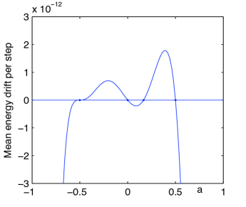
Figure 3: Measured rate of energy drift for $H=p-p^{3}+q^{2}-q^{3}$ for Runge–Kutta methods $x^{\prime}=x+h(af(x)+(1-2a)f((x+x^{\prime})/2)+af(x^{\prime}))$, varying the parameter $a$. The step size is $h=0.3$ and the initial condition is $q=0.323$, $p=1/\sqrt{3}$. All methods have an approximate modified energy up to $h^{4}$. The energy drift is measured by fitting a straight line to this modified energy over $2\times 10^{6}$ time steps. Only the four methods identified by the analysis ($a=-1/2$, Kahan; $a=0$, midpoint; $a=1/6$, Simpson; and $a=1/2$, trapezoidal) show no energy drift by this measure.

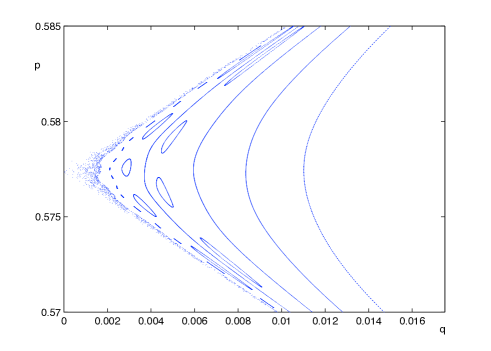
Figure 4: Portion of the phase portrait of the midpoint rule with step size $h=0.3$ applied to $H=p-p^{3}+q^{2}-q^{3}$. The observed chaotic bands and island chains indicate that it does not have a conserved quantity.

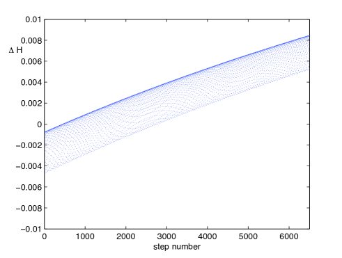
Figure 5: Suzuki’s 3-stage, 4th-order composition applied to Kahan’s method shows a comparatively rapid energy drift, indicating that there is no conserved quantity. Here $H=p-p^{3}+q^{2}-q^{3}$, $h=0.2$, and $(q_{0},p_{0})=(0.323,1/\sqrt{3})$.

4 Discussion

Level sets of $\widetilde{H}$ are shown in Figure 1 for $H=\frac{1}{2}(q^{2}+p^{2})+q^{2}p-\frac{1}{3}p^{3}$. Notice that the separatrices persist (and are unchanged) for all $h$, but that the singular set $q^{2}+p^{2}=\frac{1}{4}+\frac{1}{h^{2}}$ moves in from infinity as $h$ increases and alters the topology of the level sets. For $h<\sqrt{4/3}$ the topology of the bounded orbits is unaltered.

The bounded orbits of Figure 1 are symmetric, so for the following numerical experiments we used $H=p-p^{3}+q^{2}-q^{3}$, which has bounded, nonsymmetric orbits, an elliptic fixed point at $(q,p)=(2/3,1/\sqrt{3})$, and a separatrix meeting $(q,p)=(0,1/\sqrt{3})$. Level sets of $\widetilde{H}$ for this case are shown in Figure 2.

Numerical experiments strongly indicate that the following observations hold.

1. No other method of the family (9) has a modified Hamiltonian when $H$ is cubic, apart from the known cases $a=0$, $\pm\frac{1}{2}$, and $\frac{1}{6}$ (see Figure 3).

2. The midpoint and trapezoidal rules do not have a first integral for all cubic $H$ (even though they do have a formal invariant close to $H$) (see Figure 4).

3. Simpson’s method is not measure-preserving for all cubic $H$. (For $H=p-p^{3}+q^{2}-q^{3}$, a numerical calculation finds eigenvalues $1,\lambda$ of periodic orbits, with $\lambda\neq 1$, contradicting measure preservation.)

4. Kahan’s method does not preserve any symplectic form in dimension $\geq 4$ for all cubic $H$. (A numerical calculation of periodic points finds eigenvalues that do not occur in $\lambda$, $1/\lambda$ pairs. Proposition 2 establishes this for a limited class of symplectic forms.)

5. Compositions of Kahan’s method with different step sizes do not have a modified Hamiltonian when $H$ is cubic (see Figure 5).

Our results are significant and novel for the study of both the integrability of the mappings produced by Kahan’s method and for the study of the geometric properties of Runge–Kutta methods:

• First, our results explain the integrability of the map obtained when Kahan’s method is applied to some of the examples of [10]: their Eq. (4.2) ($H=y^{2}/2-2x^{3}+\alpha x$); Eq. (5.4) ($H=y(3x^{2}-y)$); Eq. (8.1) (Volterra chain in $\mathbb{R}^{3}$, $H=x_{1}x_{2}x_{3}$, constant $K$, integral $H_{2}$ in Eq. (8.6) is a function of our $\widetilde{H}$ and the Casimir $x_{1}+x_{2}+x_{3}$); Eq. (9.1) (Dressing chain in $\mathbb{R}^{3}$, $H=(x_{1}+x_{2})(x_{2}+x_{3})(x_{3}+x_{1})-\sum_{i}\alpha_{i}x_{i}$, constant $K$). Our results explain the invariant measure and cubic integral of their Eq. (11.1) (three wave system in ${\mathbb{C}}^{3}$, $H=z_{1}z_{2}z_{3}+\bar{z}_{1}\bar{z}_{2}\bar{z}_{3}$), the invariant measure for the family of systems in their Prop. 1, and the linear integrals throughout [10].

• Second, our results (e.g. Corollary 6) systematically produce new integrable cases of Kahan’s method.

• Third, we have shown that Kahan’s method in dimension 4 and greater provides examples of maps with nonlinear integrals and conserved measures unrelated (in general) to integrability or obvious symmetries, again a novel feature. For example, our results imply that Kahan’s application of the method to the Korteweg–de Vries equation in [9] preserves a measure and a modified energy (but the higher order compositions of the method in [9] probably do not).

• Fourth, we have shown that Kahan’s method has novel properties previously unknown amongst Runge–Kutta methods, indeed amongst all B-series. It is known that B-series methods cannot conserve the measure $dx_{1}\wedge\dots\wedge dx_{n}$ even for linear vector fields [7]; Kahan’s method circumvents this by conserving a modified measure. It is a novel conjugate-to-energy preserving method for cubic $H$. In the plane, it is also conjugate to symplectic. Thus, while no conjugate to symplectic methods are known that are also energy preserving in general, here we have one that preserves at least a modified energy, and preserves it exactly (not merely as a formal invariant).

On the other hand, there are open questions in all of these areas. While it was already suggested in [10] that there could be an underlying ‘integrability mechanism’ unifying the integrable cases, here we have unified only some of these. In addition the hoped-for unification should now be extended to include non-integrable cases preserving a measure and/or some integrals as well. On the numerical side, it is not known precisely which Runge–Kutta or B-series methods share the properties of Kahan’s method, if any are higher order integrators, or if any are conservative for nonquadratic (e.g. other polynomial) vector fields.

References

References

• [1] Bruschi M, Ragnisco O, Santini PM, and Gui-Zhang T 1991, Integrable symplectic maps, Physica D 49 273–294.
• [2] Celledoni E, McLachlan RI, McLaren DI, Owren B, Quispel GRW, and Wright W 2009, Energy-preserving Runge–Kutta methods, Mathematical Modelling and Numerical Analysis 43 645–649.
• [3] Duistermaat JJ 2010, Discrete Integrable Systems: QRT Maps and Elliptic Surfaces, Springer, Heidelberg.
• [4] Hairer E, Lubich C, and Wanner G 2006, Geometric Numerical Integration: Structure-Preserving Algorithms for Ordinary Differential Equations, 2nd ed., Springer, Berlin.
• [5] Hirota R and Kimura K 2000, Discretization of the Euler top, J. Phys. Soc. Jap. 69 627–630.
• [6] Hone ANW and Petrera M 2009, Three-dimensional discrete systems of Hirota–Kimura type and deformed Lie–Poisson algebras, J. Geom. Mech. 1 55–85.
• [7] Iserles A, Quispel GRW, and Tse PSP 2007, B-series methods cannot be volume-preserving, BIT 47 351–378.
• [8] Kahan W 1993, Unconventional numerical methods for trajectory calculations, Unpublished lecture notes.
• [9] Kahan W and Li R-C 1997, Unconventional schemes for a class of ordinary differential equations—with applications to the Korteweg–de Vries equation, J. Comput. Phys. 134 316–331.
• [10] Petrera M, Pfadler A, and Suris YB 2011, On integrability of Hirota–Kimura type discretizations, Regular and Chaotic Dynamics 16 245–289.