Warps, Bending and Density Waves Excited by Rotating Magnetized Stars: Results of Global 3D MHD Simulations

Abstract

We report results of the first global three-dimensional (3D) magnetohydrodynamic (MHD) simulations of the waves excited in an accretion disc by a rotating star with a dipole magnetic field misaligned from the star’s rotation axis (which is aligned with the disc axis). The main results are the following: (1) If the magnetosphere of the star corotates approximately with the inner disc, then we observe a strong one-armed bending wave (a warp). This warp corotates with the star and has a maximum amplitude between corotation radius and the radius of the vertical resonance. The disc’s center of mass can deviate from the equatorial plane up to the distance of $z_{w}\approx 0.1r$. However, the effective height of the warp can be larger, $h_{w}\approx 0.3r$ due to the finite thickness of the disc. Stars with a range of misalignment angles excite warps. However, the amplitude of the warps is larger for misalignment angles between $15$ and $60$ degrees. The location and amplitude of the warp does not depend on viscosity, at least for relatively small values of the standard alpha-parameter, up to $0.08$. (2) If the magnetosphere rotates slower, than the inner disc, then a bending wave is excited at the disc-magnetosphere boundary, but does not form a large-scale warp. Instead, persistent, high-frequency oscillations become strong at the inner region of the disc. These are (a) trapped density waves which form inside the radius where the disc angular velocity has a maximum, and (b) inner bending waves which appear in the case of accretion through magnetic Rayleigh-Taylor instability. These two types of waves are connected with the inner disc and their frequencies will vary with accretion rate. Bending oscillations at lower frequencies are also excited including global oscillations of the disc. In cases where the simulation region is small, slowly-precessing warp forms with the maximum amplitude at the vertical resonance. The present simulations are applicable to young stars, cataclysmic variables, and accreting millisecond pulsars. A large-amplitude warp of an accretion disc can periodically obscure the light from the star. Different types of waves can be responsible for both the high and low-frequency quasi-periodic oscillations (QPOs) observed in different types of stars. Inner disc waves can also leave an imprint on frequencies observed in moving hot spots on the surface of the star.

1 Introduction

Different types of accreting stars have dynamically important magnetic fields, such as young T Tauri stars (e.g., Bouvier et al. 2007a), accreting millisecond pulsars (e.g., van der Klis 2000, 2006), and accreting white dwarfs (e.g., Warner 1995, 2004).

If a rotating star has a tilted dipole (or other non-axisymmetric) magnetic field then it applies a periodic force on the inner part of the accretion disc and different types of waves are excited and propagate to larger distances (e.g., Lai 1999). The linear theory of waves in discs has been developing extensively over many years (see, e.g., book by Kato et al. 1998 and references therein). If an external force is applied to the disc from the tilted dipole of a rotating star (or from a secondary star or planet), then this force can generate density waves in the disc (e.g., Goldreich 1978) and vertical bending waves (e.g., Lubow 1981; Lai 1999; Ogilvie 1999). Theoretical investigations have led to an understanding that both types of waves may be strongly enhanced or damped at radii corresponding to resonances (e.g., Kato et al. 1998). There are two types of resonances: horizontal resonance (Lindblad resonance) and vertical resonance. Another important resonance is associated with corotation radius $r_{\rm cr}$ where the angular velocity of the disc matches the angular velocity of the external force.

Aly (1980) and Lipunov (1980) investigated the tilting of the inner disc due to the magnetic force applied by the rotating dipole magnetosphere of the star where both the magnetic and rotational axes of the star are misaligned relative to the rotational axis of the outer disc. They concluded that the magnetic force acting on the inner disc causes it to strongly depart from the original plane of the disc. Lai (1999) investigated this case and concluded that the magnetic force also drives a warp at the inner disc which slowly precesses around the rotational axis of the disc.

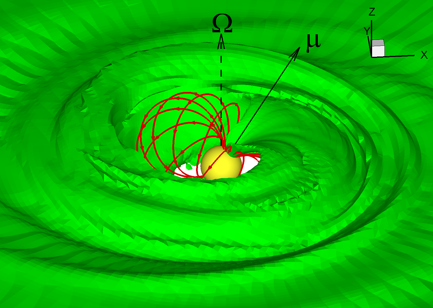
Figure 1: An example of the magnetospheric accretion and a warp driven by the rotating and tilted at $\theta=30^{\circ}$ dipole magnetosphere with $\tilde{\mu}=1.5$ (model FW$\mu$1.5). The background shows one density level ($\rho=0.07$). The lines are sample magnetic field lines of the closed magnetosphere. The vectors $\bf{\mu}$ and $\bf{\Omega}$ show directions of the magnetic and rotational moments of the star.

Terquem & Papaloizou (2000) investigated the formation of a disc warp in the case where the rotational axis of the star is aligned with that of the disc, and the inner disc corotates with the star, taking into account an $\alpha-$type viscosity in the disc (Shakura & Sunyaev, 1973). They concluded that for a relatively small viscosity, $\alpha=0.01-0.08$, a warp is excited near the magnetosphere and corotates with the star. However, it is suppressed by the viscosity at larger distances from the star. They also concluded that the height of the warp can reach up to $\sim 10\%$ of the radial distance. One of the main motivations for studying inner disc warps comes from observations of young T Tauri stars (CTTS) in which the light curves show regular dips that can be interpreted as obscuration events by a warped disc (e.g., Bouvier et al. 1999, 2003, 2007b, also Carpenter et al. 2001).

Another important impetus to study waves in the disc comes from observations of quasi-periodic oscillations (QPOs) in different accreting stars: neutron stars, black holes, and white dwarfs. For example, in low-mass X-ray binaries (LMXBs), typical QPO frequencies vary from very high, $\nu\approx 1300$Hz, down to very low, $\nu\sim 0.1$Hz (e.g., van der Klis 2006). An important feature of the spectra is the presence of ‘twin peaks’ of high-frequency QPOs. In many cases, the separation between peaks is equal to either the frequency of the star or half of its value (e.g., van der Klis 2000). Different theories have been proposed to explain this phenomenon (e.g., Lamb et al. 1985; Miller, Lamb & Psaltis 1998; Lovelace & Romanova 2007). In a number of accreting millisecond pulsars, the difference between peaks does not correlate with the frequency of the star and varies in time significantly (e.g., Sco X-1), and this also requires an explanation (e.g., van der Klis et al. 1997).

In accreting magnetized stars, the magnetosphere may rotate slower than the inner disc (e.g., Romanova et al. 2002, Long et al. 2005). Consequently, there is a maximum in the angular velocity distribution as a function of radius at the inner disc. This condition can lead to formation of unstable radially trapped Rossby waves (Lovelace & Romanova, 2007; Lovelace et al., 2009). These waves can be responsible for one of the high-frequency QPO peaks observed in LMXBs. These waves may play a role of blobs suggested earlier in theoretical models of QPOs, such as in the beat-frequency model (e.g., Miller, Lamb & Psaltis 1998; Lamb & Miller 2003). However, compared with the blobs, the inner density waves are much more ordered, and have higher coherence. However, the origin of the second QPO peak is still unclear.

Different QPO frequencies in discs around stars and black holes can be connected with resonances in the disc, where the amplitude of waves may be enhanced (e.g., Kato et al. 1998; Kato 2004; Zhang & Lai 2006). For example, Lamb & Miller (2003) and Lai & Zhang (2008) suggest that wave can be excited at the spin-orbital resonance, and the light from the high-frequency QPO can interact with this wave and result in the lower-frequency QPO. Kato (2004) suggested that in the case of the tilted black holes the disc may be warped, and investigated resonance associated with non-linear interaction of different waves with this warp (see also Petri 2005; Lai & Zhang 2008; Kato 2008, 2010). Slowly-precessing warps can form in both the black hole and the magnetic star cases and can be responsible for low-frequency QPOs (e.g., Lai 1999; Pfeiffer & Lai 2004).

The very low-frequency oscillations ($\sim 0.1-1$Hz) in LMXBs can be connected with disc oscillations at large distances form the star (e.g., corrugation waves can be excited, Kato et al. 1998). Such global oscillations have been observed in numerical simulations of accretion to a black hole with a tilted spin axis (Fragile & Anninos, 2005; Fragile et al., 2007). The authors note that the frequency of these oscillations depends strongly on the size of the disc.

In all above-mentioned cases, where a rotating magnetized star excites waves in a disc, the waves have been analyzed using linearized equations. The linear theory provides an important theoretical understanding of the different waves. However, the approach has significant limitations, particularly in those cases where the amplitude of waves is not small. Further, the theory gives only a rough treatment of the force on a disc due to a tilted stellar magnetic field. In this paper, we present the first results of global three-dimensional (3D) MHD simulations of waves excited by a rotating star with a misaligned dipole magnetic field. Earlier, we investigated the magnetospheric flow around tilted dipoles (e.g., Romanova et al. 2003, 2004), and motion of hot spots at the stellar surface (e.g., Romanova et al. 2008; Kulkarni & Romanova 2009; Bachetti et al. 2010). However, this is the first time when we investigate waves in the disc which are excited by a rotating tilted dipole.

In Sec. 2 we briefly describe the linear theory of waves in discs, our numerical model and methods for wave analysis in simulations. We also discuss the theory of waves in Keplerian discs in Appendix A and the theory of trapped waves in Appendix B. In Sec. 3 we present the results of our simulations. We discuss applications of the numerical results in Sec. 4. Conclusions are given in Sec. 5.

2 The model, and analysis of waves in the disc

Below we give the highlights of the linear theory of waves (Sec. 2.1), describe our numerical model (Sec. 2.2) and the approach which has been used for analysis of waves in numerical simulations (Sec. 2.3).

2.1 Theoretical background

Here we briefly summarize the theory of waves excited in accretion discs (see, e.g., Kato et al. 1998). In the majority of theoretical studies, the disc is approximated to be thin, isothermal and non-magnetic. Furthermore, oscillations can be free, or can be excited by the external force. Below we briefly discuss different types of waves.

2.1.1 Free oscillations in the disc

Small perturbations of a thin, non-magnetized disc involve in-plane and out-of-plane displacements of the disc matter. Waves can be roughly divided into inertial-acoustic waves (referred to as p-modes, where the restoring forces are rotation and pressure gradient), and and inertial-gravity waves, referred to as g-modes where the restoring force is gravity Inertial-acoustic modes are in-plane modes, and they propagate in the form of pressure or density disturbances. They are often termed “density waves” (see also Goldreich 1978). The inertial-gravity modes are out-of-plane modes (Kato et al., 1998). These waves lead to misplacement of the local center of mass of the disc out of the equatorial plane and hence are called “bending waves”.

For both the in-plane and out-of-plane modes, the azimuthal dependence is $\exp(im\phi)$, with $m=0,~{}1,~{}2,..$. The $m=1$ in-plane perturbation is a one-armed spiral wave and the $m=2$ in-plane mode is a two-armed spiral wave. The out-of-plane modes involve a small vertical displacement or shift of the midplane of the disc, $z_{w}(t,r,\phi)$ (cylindrical coordinates) with $|z_{w}|\ll r$.

To investigate the propagation of small-amplitude waves in the disc, perturbations of the hydrodynamical values $Q=p,~{}\rho,~{}v_{r},..$ are expanded as (e.g., Okazaki et al. 1987; Tanaka et al. 2002; Lai & Zhang 2008):

$$Q(r,z,\phi,t)=\sum_{m,n,\omega}Q_{m,n,\omega}(r)H_{n}\left(\frac{z}{h}\right)\exp(im\phi-i\omega t)~{}.$$ (1)

Here, $\omega$ is the angular frequency of the wave, $m=0,~{}1,~{}2...$ is the number of arms in the azimuthal direction, $H_{n},n\geq 0$ are the Hermite polynomials (with $n=0,~{}1,~{}2,..$), and $h(r)$ is the half-thickness of the disc at radius $r$. Waves with $n=0$ and $n=1$ represent density and bending waves, respectively.

Linearization of the equations of motion (e.g., Kato et al. 1998) leads to

$$\frac{d^{2}\psi}{dr^{2}}+\frac{(\tilde{\omega}^{2}-\kappa^{2})(\tilde{\omega}^{2}-n\Omega_{\perp}^{2})}{c_{s}^{2}\tilde{\omega}^{2}}\psi=0~{},$$ (2)

where $\psi=\delta p/\rho_{0}$ is the perturbation of the enthalpy for density waves or $z_{w}$ for the bending waves. Also in this equation, $\tilde{\omega}\equiv\omega-m\Omega$ is the Doppler-shifted angular frequency of the wave seen by an observer orbiting at the disc’s angular velocity $\Omega(r)$, $\Omega_{\perp}$ is the frequency of oscillations perpendicular to the disc, $\kappa^{2}=r^{-3}d(r^{4}\Omega^{2})/dr$ is the square of the radial epicyclic frequency, and $c_{s}$ is the sound speed in the disc.

The local free wave solution in the WKBJ approximation can be considered as (Kato et al. 1998),

$$\psi\propto k_{r}^{-1/2}\exp\big{[}i\int^{r}drk_{r}(r)\big{]}~{},$$ (3)

for $(k_{r}r)^{2}\gg 1$ and $(k_{r}h)^{2}\ll 1$, where $k_{r}$ is the radial wavenumber. Thus, equation (2) can be presented as $d^{2}\psi/dr^{2}=-k_{r}^{2}\psi$ and one gets the dispersion relation:

$$\frac{(\tilde{\omega}^{2}-\kappa^{2})(\tilde{\omega}^{2}-n\Omega_{\perp}^{2})}{\tilde{\omega}^{2}}=k_{r}^{2}c_{s}^{2}~{}.$$ (4)

Propagation of the perturbations is possible in regions where $(\tilde{\omega}^{2}-\kappa^{2})(\tilde{\omega}^{2}-n\Omega_{\perp}^{2})>0$. The WKBJ approximation breaks down in the vicinity of points where the coefficient of $\psi$ in equation (2) changes sign or has a singularity. At the points where $\tilde{\omega}=\pm\kappa$ there is an outer (+sign) or an inner (-sign) Lindblad resonance. At the points where $\tilde{\omega}=\pm n\Omega_{\perp}$ (for $n\neq 0$) there are vertical resonances. For $\tilde{\omega}=0$ there is a corotation resonance. Appendix A summarizes the behavior of these different modes.

In this work we are mainly interested in (1) oscillations in the plane of the disc ($n=0$), and (2) out of plane oscillations ($n=1$). Further, we consider only the one-armed ($m=1$) and two-armed ($m=2$) modes. If the accretion disc is Keplerian, then $\kappa=\Omega_{\perp}=\Omega$. From the analysis of Zhang & Lai (2006), one-armed density waves ($m=1$) at $n=0$ can propagate only in the region of the disc outside the outer Lindblad resonance. The inner Lindblad and corotational resonances in this case ($n=0$) are absent. For vertical oscillations ($n=1$), the position of the outer Lindblad and vertical resonances coincide. Two-armed density waves ($m=2$) with $n=0$ can propagate either in the external parts of the disc outside the outer Lindblad resonance or in the region inside the inner Lindblad resonance.

	CTTSs	White dwarfs	Neutron stars
$M(M_{\odot})$	0.8	1	1.4
$R_{*}$	$2R_{\odot}$	5000 km	10 km
$B_{*}$ (G)	$10^{3}$	$10^{6}$	$3\times 10^{8}$
$R_{0}$ (cm)	$4\times 10^{11}$	$1.4\times 10^{9}$	$2.9\times 10^{6}$
$v_{0}$ (cm s-1)	$1.6\times 10^{7}$	$3\times 10^{8}$	$8.1\times 10^{9}$
$\rho_{0}$ (g cm-3)	$2.8\times 10^{-11}$	$7.9\times 10^{-8}$	$1.0\times 10^{-5}$
$\sigma_{0}$ (g cm-2)	$11.0$	$112.5$	$28.9$
$\nu_{0}$	$0.55$ day-1	$3.2\times 10^{-2}$ Hz	$4.5\times 10^{2}$ Hz
$P_{0}$	$1.8$ days	29 s	2.2 ms

Table 1: Sample values of the physical parameters of different types of stars. See Sec. 2.2 for a description.

2.1.2 Waves excited by the external force. Resonances

In our model, waves are ‘driven’ by the rotating tilted magnetosphere of the star. The interaction of the magnetosphere with the disc is a complex, non-linear, and non-stationary process. For simplicity of the analysis, this interaction can be approximated by the force acting on the disc and presented as a sum of different harmonics:

$$f=f(r,z,\phi-\Omega_{*}t)=\sum_{m}f_{m}(r,z)\exp[im(\phi-\Omega_{*}t)]~{},$$ (5)

where $\Omega_{*}$ is the angular frequency of the star. In linear approximation, we suggest that the $m-$harmonic of this force excites the $m-$armed wave in the disc. The frequency of this force is $m\Omega_{*}$. Then, for a Keplerian disc, the condition for the Lindblad resonances $\tilde{\omega}=\pm\Omega$ will be $m\Omega_{*}-m\Omega=\pm\Omega$, or

$$r_{LR}=r_{cr}\bigg{(}1\pm\frac{1}{m}\bigg{)}^{2/3}~{},$$ (6)

where $r_{cr}=(GM/\Omega_{*}^{2})^{1/3}$ is the corotation radius. For bending waves, $n=1$, the condition for vertical resonances $\tilde{\omega}=\pm\Omega$ is the same, and hence the vertical resonances are located at the same radii.

For a one-armed density wave ($m=1$, $n=0$) in a Keplerian disc, the outer Lindblad resonance is located at radius $r_{\rm OLR}=(4GM/\Omega_{*}^{2})^{1/3}$. The location of the outer vertical resonance $r_{\rm OVR}$ for a bending wave ($n=1$) is the same. For a two-armed spiral wave ($m=2$), the outer Lindblad and vertical resonances are located at the distance of $r_{\rm OLR}=r_{\rm OVR}=[9GM/(4\Omega_{*}^{2})]^{1/3}$, while the inner Lindblad resonance is at the distance $r_{\rm ILR}=r_{\rm IVR}=[GM/(4\Omega_{*}^{2})]^{1/3}$. The corotation resonance for all waves is located at radius $r_{\rm CR}=(GM/\Omega_{*}^{2})^{1/3}$. A more detailed description of the modes is given in Appendix A. In this paper we compare position of waves observed in simulations with position of resonances derived theoretically.

2.1.3 High-frequency trapped waves near magnetized stars

In relativistic discs, the epicyclic frequency $\kappa$ has a maximum at the inner disc (where relativity effects from a black hole or a neutron star are stronger), and this may lead to formation of waves which are trapped below this maximum (e.g., Okazaki et al. 1987; Nowak & Wagoner 1991; Kluzniak & Abramowicz 2002). These waves are important because they may be responsible for the high-frequency QPOs observed in black hole-hosting systems (e.g., Stella & Vietri 1999; Alpar & Psaltis 2005, 2008).

In cases where a star has a dynamically-important magnetic field and is slowly rotating, the magnetosphere slows down the rotation of matter at the inner part of the disc. Hence, there is a maximum in the disc angular velocity distribution. This situation is similar to that of relativistic discs: high-frequency waves can be trapped below the maximum of the angular velocity distribution (e.g., Lovelace & Romanova 2007; Lovelace et al. 2009). We briefly summarize the theory of trapped waves around magnetized stars in Appendix B.

2.1.4 Low-frequency bending waves

In the absence of an external force, perturbation of the disc in the vertical direction leads to the formation of free bending waves. Namely, the matter lifted above the equatorial plane ($z=0$) to the height $z$ experiences the restoring gravity force $g=-GM_{*}z/r^{3}$ per unit mass. That is why the frequency of matter oscillation in the vertical direction is $\Omega_{\perp}\approx\Omega=\sqrt{GM/r^{3}}$, therefore, at large distances from the star, these oscillations have a very low frequency. A one-arm global bending wave with low frequency and long wavelength in the radial direction (or, corrugation wave) can propagate to very large radial distances (Kato et al., 1998). In addition, global bending oscillations of the whole disc are possible. Waves can also be reflected or generated at the outer boundary of the disc (Zhang & Lai, 2006). Such low-frequency oscillations can be excited by the rotating magnetosphere of the star, in particular if the star rotates slowly.

2.1.5 More realistic discs

Real accretion discs have a finite thickness, and hence the thin disc approximation may not be applicable. In addition, the disc may have a complex distribution of density, temperature and magnetic field. All these factors may determine the formation and propagation of waves (e.g., Kato et al. 1998, Fu & Lai 2012).

Waves in discs of finite thickness were investigated in few global 3D simulations of accretion onto rotating black holes with the tilted spin. Formation of warp and tilted discs have been observed in these simulations (e.g., Nelson & Papaloizou 2000; Fragile & Anninos 2005). Different disco-seismic modes (such as trapped g-mode), were observed in axisymmetric simulations of accretion on to a non-rotating black hole from non-magnetized accretion disc (e.g., O’Neil et al. 2009). However, in discs where accretion is driven by the magneto-rotational instability (MRI, e.g., Balbus & Hawley 1991), no interesting waves, such as trapped relativistic g-modes were observed (e.g., Reynolds & Miller 2009). These simulations show that the magnetic field may possibly damp waves in the disc.

In our simulations, the disc has a finite thickness, $h/r\approx 0.1$, which approximates a thin disc. We observed in simulations that the angular velocity is almost Keplerian in major part of the disc (excluding the inner parts near the magnetosphere) and hence the approximation for Keplerian disc is valid. Some magnetic flux of the magnetosphere is trapped inside the disc and hence may influence the positions of resonances. However, this is the region where the angular velocity is strongly non-Keplerian, and where we can not apply the standard theory of waves. Overall, results obtained in our model can be compared with results obtained with the linear theory of waves in a thin disc, excluding the innermost region of the disc, where the theory of trapped waves (Lovelace & Romanova, 2007; Lovelace et al., 2009) is more appropriate.

Name	$\widetilde{\mu}$	$r_{\rm cor}$	$\Omega_{*}$	$\theta$	$\alpha$	$R_{\rm out}/R_{*}$	Warp Properties
FW$\mu$0.5	0.5	1.5	0.54	$30^{\circ}$	$\alpha=0.02$	34.5	fast, $\Omega_{w}\approx\Omega_{*}$
FW$\mu$1.5	1.5	1.8	0.41	$30^{\circ}$	$\alpha=0.02$	34.5	fast, $\Omega_{w}\approx\Omega_{*}$
FW$\theta$5	0.5	1.5	0.54	$5^{\circ}$	$\alpha=0.02$	34.5	fast, $\Omega_{w}\approx\Omega_{*}$
FW$\theta$15	0.5	1.5	0.54	$15^{\circ}$	$\alpha=0.02$	34.5	fast, $\Omega_{w}\approx\Omega_{*}$
FW$\theta$45	0.5	1.5	0.54	$45^{\circ}$	$\alpha=0.02$	34.5	fast, $\Omega_{w}\approx\Omega_{*}$
FW$\theta$60	0.5	1.5	0.54	$60^{\circ}$	$\alpha=0.02$	34.5	fast, $\Omega_{w}\approx\Omega_{*}$
FW$\theta$90	0.5	1.5	0.54	$90^{\circ}$	$\alpha=0.02$	34.5	fast, $\Omega_{w}\approx\Omega_{*}$
FW$\alpha$0.00	0.5	1.5	0.54	$30^{\circ}$	$\alpha=0.00$	34.5	fast, $\Omega_{w}\approx\Omega_{*}$
FW$\alpha$0.04	0.5	1.5	0.54	$30^{\circ}$	$\alpha=0.04$	34.5	fast, $\Omega_{w}\approx\Omega_{*}$
FW$\alpha$0.06	0.5	1.5	0.54	$30^{\circ}$	$\alpha=0.06$	34.5	fast, $\Omega_{w}\approx\Omega_{*}$
FW$\alpha$0.08	0.5	1.5	0.54	$30^{\circ}$	$\alpha=0.08$	34.5	fast, $\Omega_{w}\approx\Omega_{*}$
SWcor1.8	0.5	1.8	0.41	$30^{\circ}$	$\alpha=0.02$	34.5	slow, $\Omega_{w}\approx 0.5\Omega_{*}$
SWcor3	0.5	3.0	0.19	$30^{\circ}$	$\alpha=0.02$	34.5	slow, $\Omega_{w}\approx 0.1\Omega_{*}$
SWcor5	0.5	5.0	0.09	$30^{\circ}$	$\alpha=0.02$	34.5	slow, $\Omega_{w}\approx 0.02\Omega_{*}$
LRcor1.8	0.5	1.8	0.41	$30^{\circ}$	$\alpha=0.02$	57.7	no big warp
LRcor3	0.5	3.0	0.19	$30^{\circ}$	$\alpha=0.02$	57.7	no big warp
LRcor5	0.5	5.0	0.09	$30^{\circ}$	$\alpha=0.02$	57.7	no big warp
SRcor3	0.5	3.0	0.19	$30^{\circ}$	$\alpha=0.02$	26.9	disc oscillations, example

Table 2: The main set of simulation runs. See Sec. 3.1 for a detailed description.

				$\bf{m=1}$					$\bf{m=2}$
$\Omega_{*}$	$r_{\rm CR}$			$r_{\rm OLR}$	$r_{\rm OVR}$			$r_{\rm ILR}$	$r_{\rm OLR}$	$r_{\rm IVR}$	$r_{\rm OVR}$
				$n=0$	$n=1$			$n=0$	$n=0$	$n=1$	$n=1$
$0.544$	1.5			2.38	2.38			0.94	1.97	0.94	1.97
$0.414$	1.8			2.86	2.86			1.13	2.36	1.13	2.36
$0.192$	3.0			4.76	4.76			1.89	3.93	1.89	3.93
$0.089$	5.0			7.93	7.93			3.15	6.55	3.15	6.55

Table 3: Radii of resonances in a thin hydrodynamic Keplerian disc excited by a rotating perturbation from a magnetized star rotating with angular velocity $\Omega_{*}$ (in dimensionless units discussed in the text). $r_{\rm CR}$ is the radius of the corotation resonance. The next two columns show the radii of the outer Lindblad $r_{\rm OLR}$ and outer Vertical $r_{\rm OVR}$ resonances in the case of one-armed ($m=1$) density ($n=0$) and bending ($n=1$) waves. The right four columns show the radii for resonances in the cases of two-arm waves: inner and outer Lindblad resonances $r_{\rm ILR}$ and $r_{\rm OLR}$ for density waves ($n=0$), and inner and outer vertical resonances $r_{\rm IVR}$ and $r_{\rm OVR}$ for bending waves ($n=1$).

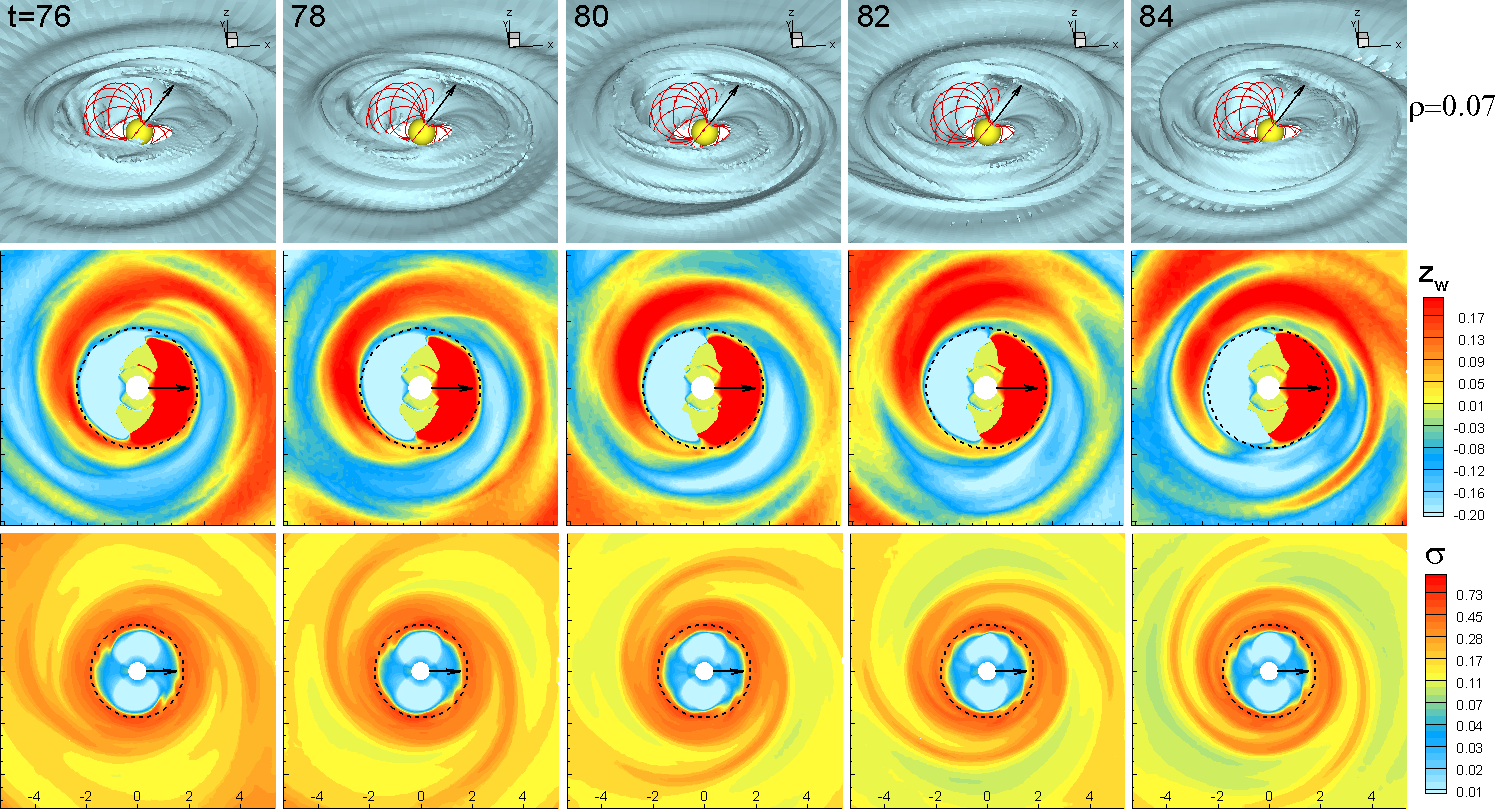
Figure 2: Views of the inner parts of the disc in a model with a relatively large magnetic moment, $\widetilde{\mu}=1.5$ (model FW$\mu$1.5) at different times, $t$. Top row: A three-dimensional view of the disc at one density level, $\rho=0.07$. Middle row: $z-$averaged height of the disc’s center of mass above or below the equatorial plane, $z_{w}$. Bottom row: surface density distribution in the equatorial plane, $\sigma$. Time $t$ is given in units of $P_{0}/4$, where $P_{0}$ is the orbital period at $r=1$. Plots are shown in a coordinate system rotating with the star.

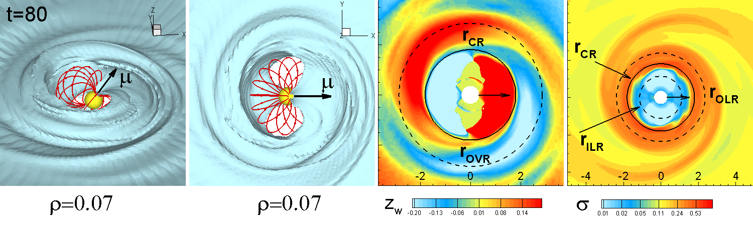
Figure 3: Views of bending and density waves shown in Fig. 2 at time $t=80$. The left two panels show 3D views of the warp from the side and face-on orientations. The right two panels show bending and density waves and the locations of resonances: $r_{\rm CR}$ is the corotation resonance; $r_{\rm OVR}$ is the outer vertical resonance (calculated for $m=1$); $r_{\rm ILR}$ and $r_{\rm OLR}$ are the inner and outer Lindblad resonances respectively (calculated for $m=2$). Plots are shown in a coordinate system rotating with the star. Positions of resonances are taken from Tab. 3.

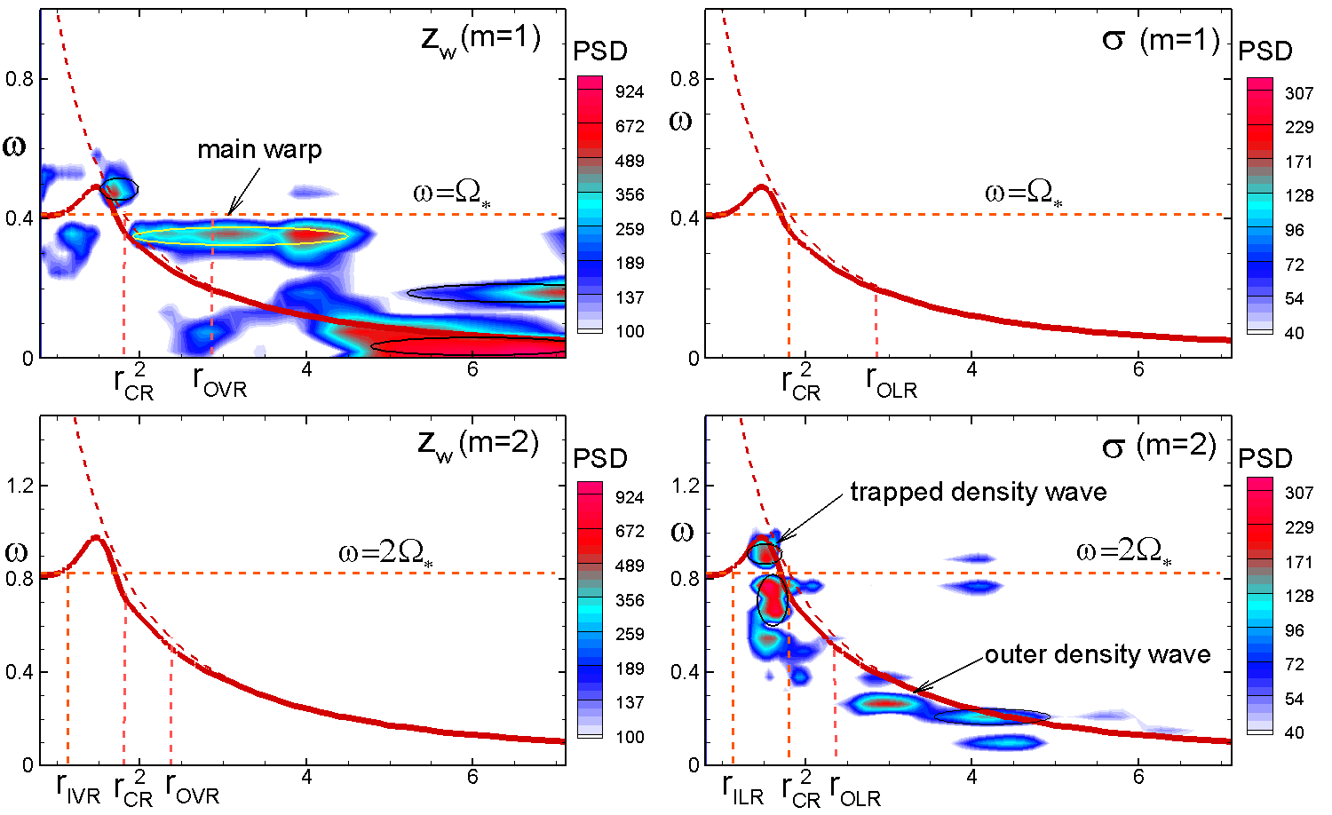
Figure 4: Power spectral density (PSD) obtained for waves in model FW$\mu$1.5 inside $r<7$ of the simulation region (the entire region is $R_{\rm out}=12.1$). Left panels: PSD for one-armed, $m=1$, (top) and two-armed, $m=2$, (bottom) bending waves. Right panels: same, but for density waves. The solid red lines show the angular velocity distribution in the disc. Dashed lines show angular frequency of the star and positions of resonances. All frequencies are given in the non-rotating reference frame. Position of resonances is taken from Tab. 3.

2.2 Numerical model and reference values

We solve the 3D MHD equations with a Godunov-type code in a reference frame rotating with the star, using the “cubed sphere” grid. The model has been described earlier in a series of previous papers (e.g., Koldoba et al. 2002; Romanova et al. 2003, 2004). Hence, we will describe it only briefly here.

Initial conditions. A rotating magnetic star is surrounded by an accretion disc and a corona. The disc is cold and dense, while the corona is hot and rarefied, and at the reference point (the inner edge of the disc in the disc plane), $T_{c}=100T_{d}$, and $\rho_{c}=0.01\rho_{d}$, where subscripts ‘d’ and ‘c’ denote the disc and the corona, which are initially in rotational hydrodynamic equilibrium (see e.g., Romanova et al. 2002 for details). The disc is relatively thin, with the half-thickness to radius ratio $h/r\approx 0.1$.

Boundary conditions. At both the inner and outer boundaries, most of the variables $A_{j}$ are taken to have free boundary conditions, ${\partial A_{j}}/{\partial r}=0$. On the star (the inner boundary) the magnetic field is frozen onto the surface of the star. That is, the normal component of the field, $B_{n}$, is independent of time. The other components of the magnetic field vary. At the outer boundary, matter is not permitted to flow into the region. The simulation region is usually large enough that the disc has enough mass to sustain accretion flow for the duration of the simulation. The free boundary conditions on the hydrodynamic variables at the stellar surface means that accreting gas can cross the surface of the star without creating a disturbance in the flow. This also neglects the complex physics of interaction between the accreting gas and the star, which is expected to produce a strongly non-stationary shock wave in the stellar atmosphere (e.g., Koldoba et al. 2008).

A “cubed sphere” grid is used in the simulations. The grid consists of $N_{r}$ concentric spheres, where each sphere represents an inflated cube. Each of the six sides of the inflated cube has an $N\times N$ curvilinear grids which represent a projection of the Cartesian grid onto the sphere. The whole grid consists of $6\times N_{r}\times N^{2}$ cells. The typical grid used in our simulations has $N^{2}=61^{2}$ angular cells in each block. We use a different number of grid cells in the radial direction: $N_{r}=130,140,160$.

Reference values. The simulations are performed in dimensionless variables $\widetilde{A}$. To obtain the physical dimensional values $A$, the dimensionless values $\widetilde{A}$ should be multiplied by the corresponding reference values $A_{0}$ as $A=\widetilde{A}A_{0}$. These reference values include: mass $M_{0}=M_{*}$, where $M_{\star}$ is the mass of the star; distance $R_{0}=R_{*}/0.35$, where $R_{*}$ is the radius of the star ; and velocity $v_{0}=(GM/R_{0})^{1/2}$. The time scale is the period of rotation at $r=R_{0}$: $P_{0}=2\pi R_{0}/v_{0}$. Reference angular velocity is $\omega_{0}=v_{0}/R_{0}$, reference frequency is $\nu_{0}=\omega_{0}/2\pi$. To better resolve the temporal behavior of the different waves, we record the simulation data every quarter of rotation. In the figures we show time $t$ in units of $P_{0}/4$. Let $\mu_{*}=B_{*}R_{*}^{3}$ be the magnetic moment of the star, where $B_{*}$is the magnetic field at the magnetic equator. We determine the reference magnetic field $B_{0}$ and magnetic moment $\mu_{0}=B_{0}R_{0}^{3}$ such that $\mu_{0}=\mu_{*}/\widetilde{\mu}$, where $\widetilde{\mu}$ is the dimensionless magnetic moment of the star, which is used as a parameter in the code to vary the size of the magnetosphere. The reference field is $B_{0}=\mu_{*}/(R_{0}^{3}\widetilde{\mu})$, the reference density is $\rho_{0}=B_{0}^{2}/v_{0}^{2}$ and the reference mass accretion rate is $\dot{M}_{0}=\rho_{0}v_{0}R_{0}^{2}=\mu_{*}^{2}/(\widetilde{\mu}^{2}R_{0}^{4}v_{0})$. Reference surface density $\sigma=\rho_{0}R_{0}$. We use in our simulations $\widetilde{\mu}=0.5$ for most runs and $\widetilde{\mu}=1.5$ for sample runs with a larger magnetosphere. The main reference values are given in Tab. 1 for $\widetilde{\mu}=0.5$.

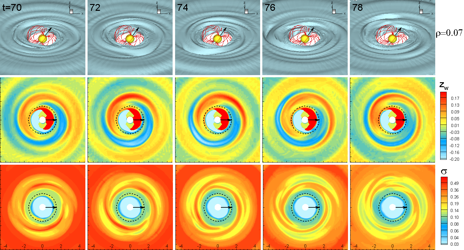
Figure 5: Same as in Fig. 2, but for a smaller magnetosphere, $\widetilde{\mu}=0.5$ (model FW$\mu$0.5).

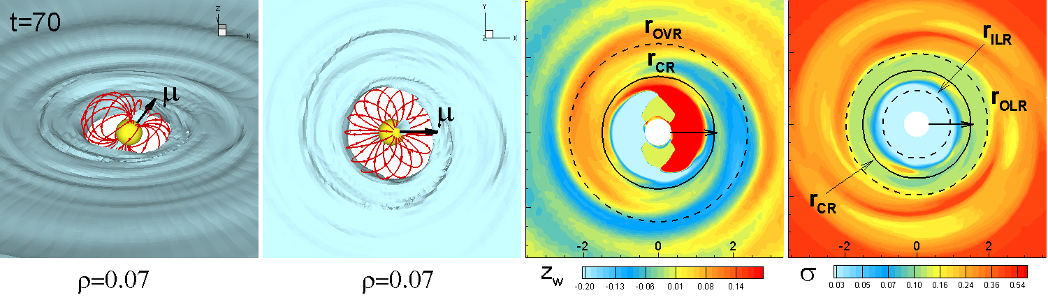
Figure 6: Same as in Fig. 3, but for a smaller magnetosphere, $\widetilde{\mu}=0.5$ (model FW$\mu$0.5).

Numerical method and code: In our Godunov scheme, we use the solver described by Powell (1999). We use a coordinate system rotating with the star. We split the magnetic field into a vacuum dipole component and a component calculated in equations: $\bf B=\bf B_{d}+\bf B^{\prime}$ (Tanaka, 1994). We solve the full set of equations for the ideal magnetohydrodynamics (e.g., Koldoba et al. 2002). Instead of using the full energy equation, we use an equation for the entropy in the form: $\partial K(S)/\partial t+(\textbf{u}\cdot\bigtriangledown)K(S)=0$, where $K(S)=p/\rho^{\gamma}$ is a function of the specific entropy $S$ . However, to characterize the thermodynamic properties of the disc, we use the temperature derived from the the ideal gas equation, $T=p/\rho{\mathcal{R}}$.

Viscosity is included in the code, with the $\alpha-$prescription for the viscosity coefficient (Shakura & Sunyaev, 1973). Viscosity supports slow, quasi-steady accretion of matter towards the star during long time intervals. The viscosity is nonzero only inside the disc, that is, above a certain threshold density (which is $\rho=0.2$ in our dimensionless units). We use small value $\alpha=0.02$ in most of the simulation runs, but take even smaller, as well as larger values in the test runs.

A typical simulation run lasts about $50P_{0}$. This time is sufficient to observe and analyze most frequencies in the disc. To analyze global, low-frequency modes in the disc, we use a smaller simulation region.

We consider only non-relativistic discs. For discs around neutron stars the relativistic effects can be important and can significantly modify the waves (e.g., Nowak & Wagoner 1991; Kato et al. 1998). However, test simulations of waves performed in the weakly relativistic case show results similar to those of the non-relativistic case.

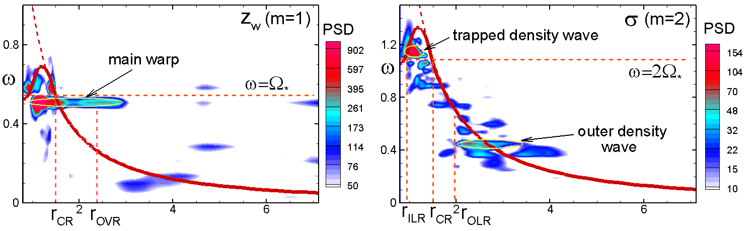
Figure 7: Power spectral density obtained for waves in model FW$\mu$0.5 inside $r<7$ of the simulation region. Left panel: PSD for one-armed, $m=1$, bending wave. Right panel: PSD for two-armed, $m=2$, density waves.

2.3 Analysis of waves in the disc

Here, we describe the methods used to analyze the different waves observed in our 3D MHD simulations.

2.3.1 Visualization of density and bending waves

To reveal the position and amplitude of density and bending waves, we separate the disc from the corona using one of the density levels, $\rho_{0}=0.03$, and then integrate through the disc in the $z-$direction.

To analyze the density waves, we calculate the surface density at each point of the disc for different moments of time:

$$\sigma=\sigma(t,r,\phi)=\int dz\rho~{},$$ (7)

where $r$ is the radius in the equatorial plane and $\phi$ is the azimuthal angle. As a result, we obtain the two-dimensional distribution of density waves.

To analyze the bending waves, we calculate the vertical displacement of the center of mass for each point of the disc:

$$z_{w}(t,r,\phi)=\frac{\int dz\rho z}{\int dz\rho}~{},$$ (8)

and obtain a two-dimensional distribution of bending waves for different times.

Typically, most of the matter in the disc has a density of $\rho=0.1$ or higher. We chose a smaller value for $\rho_{0}$ in order to be sure that we do not miss the regions between spiral waves, or other locations with low density.

We use the time-dependent distribution of $\sigma(t,r,\phi)$ and $z_{w}(t,r,\phi)$ for visualization of density and bending waves, and also for spectral analysis described in the next section.

2.3.2 Spectral analysis of disc oscillations

Here, we analyze the distribution of the angular frequencies of waves in the disc. We consider the variables $z_{w}(t,r,\phi)$ and $\sigma(t,r,\phi)$ and denote them as $f_{j}(t,r,\phi)$, $j=1,~{}2$. This is a function of time $t$, and the two spatial coordinates, $r$ (radius in the equatorial plane) and $\phi$ (azimuthal angle). Our simulations use a coordinate system rotating with the star, and the functions $f$ are calculated in this reference frame. At a fixed position ($r,~{}\phi)$ in the equatorial plane the function $f$ is quasi-periodic, because there are always some inhomogeneities in the disc which move faster or slower than the coordinate system. They cycle around the rotation axis of the disc. The function $f$ is determined in some interval of time, $t_{1}<t<t_{2}$. It is not periodic, but rather oscillates around some value, which by itself also varies in time. In addition, it rotates relative to a distant observer with the angular velocity of the star, $\Omega_{*}$. Our objective is to identify the most significant frequencies as seen by a distant observer. Also, we want to determine the distribution of waves in the disc.

As a first step of analysis, we “clean” the function $f$. The goal of this cleaning is to exclude from consideration parts of the data which are not needed for frequency analysis, for example, the average density, or regular variations of the function $f$. In general $f(t_{1})\neq f(t_{2})$, and in the observer’s frame, $f^{\rm obs}(t_{1})\neq f^{\rm obs}(t_{2})$. We consider the function which has been obtained as a result of this cleaning as a function determined for the whole time-interval $t_{2}-t_{1}$, with period $T=t_{2}-t_{1}$. In order to do this, we subtract from $f(t)$ the linear function:

$$f(t)\to f(t)-\frac{f(t_{2})-f(t_{1})}{t_{2}-t_{1}}(t-t_{1}),$$ (9)

and then subtract from the resulting function the time-averaged value

$$f(t)\to f(t)-\langle f\rangle.$$ (10)

In the next step, we select the azimuthal modes of the function $f$. The function $f^{\rm obs}$ (which is in the observer’s frame) is connected to function $f$ in the star’s frame by the relationship: $f^{\rm obs}(t,r,\phi)=f(t,r,\phi-\Omega_{*}t)$.

We use the Fourier expansion of $f^{\rm obs}$:

$$f^{\rm obs}(t,r,\phi)=\sum f_{m}^{\rm obs}(t,r)\exp(im\phi)~{},$$ (11)

where

$$f_{m}^{\rm obs}(t,r)=\frac{1}{2\pi}\int d\phi f^{\rm obs}(t,r,\phi)\exp(-im\phi)\\ =\frac{1}{2\pi}\int d\phi f(t,r,\phi-\Omega_{*}t)\exp(-im\phi)\\ =\frac{1}{2\pi}\int d\chi f(t,r,\chi)\exp[-im(\chi+\Omega_{*}t)]\\ =f_{m}(t,r)\exp(-im\Omega_{*}t).$$ (12)

In the next step, we analyze the function $f_{m}^{\rm obs}=f_{m}\exp(-im\Omega_{*}t)$. Functions $f_{m}$ and $f_{m}^{\rm obs}$ are also determined in the interval $t_{1}\leq t\leq t_{2}$. Subsequently, we perform a spectral analysis of $f_{m}$, and interpret the term $\exp(-im\Omega_{*}t)$ as the displacement of the frequency by the value $m\Omega_{*}$.

Next, we perform the time Fourier transform of $f_{m}(t,r)$. We consider $f_{m}$ as a periodic function of time with period $T=t_{2}-t_{1}$. In this case, the angular frequency has a discrete set of values with step $\delta\omega=2\pi/T$. The coefficients of the Fourier transformation are (here we neglect the numbers corresponding to frequencies):

$${\hat{f}}_{m}^{\rm obs}(\omega,r)=\frac{1}{T}\int dtf_{m}^{\rm obs}(t,r)\exp(i\omega t)\\ =\frac{1}{T}\int dtf_{m}(t,r)\exp(i\omega t-im\Omega_{*}t)={\hat{f}_{m}}(\tilde{\omega},r),$$ (13)

where, $\tilde{\omega}\equiv\omega-m\Omega_{*}$. Hence, the Fourier coefficients of the function $f_{m}(t,r)$, determined in the rotating coordinate system, are calculated for frequencies considered in the rotating coordinate system. When we transfer to the observer’s coordinate system, all frequencies are misplaced: $\omega=\tilde{\omega}+m\Omega_{*}$, but the Fourier coefficients do not change.

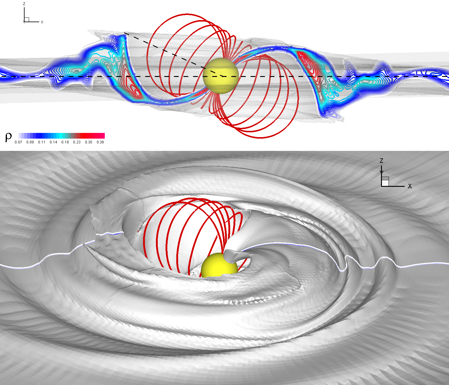
Figure 8: Analysis of the height of the warp in model FW$\mu$1.5 at $t=80$. Top panel: Cross-section of the density distribution in the $xz-$plane. Sample magnetic field lines show the location of the magnetosphere. Bottom panel: 3D view of the magnetosphere and the warp. The white line shows the location of the vertical slice shown in top panel.

To characterize the spectral properties of the function $f_{m}(t,r)$, we use the value of the Power Spectral Density (PSD):

$${\rm PSD}=|{\hat{f}}_{m}^{\rm obs}(\omega,r)|^{2}.$$ (14)

This value characterizes the power in the signal with frequency $\omega$. Here, we analyze one-armed ($m=1$) and two-armed ($m=2$) modes for density and bending waves.

3 Waves observed in 3D MHD simulations

We performed multiple simulation runs for different parameters of the star at fixed parameters of the disc (see Sec. 3.1 and Table 2). The results strongly depend on the relative positions of the magnetospheric radius, $r_{m}$ and the corotation radius, $r_{cr}$. We can separate our results into two main groups: (1) The inner disc rotates with angular velocity close to that of the star (that is, $r_{m}\approx r_{cr}$). In this case, the rotating magnetosphere excites a high-amplitude bending wave (a warp), which rotates with the angular velocity of the star (see Sec. 3.2). (2) The inner disc rotates faster than the star (that is, $r_{m}<r_{cr}$). In these models, the high-amplitude (corotating with the star) warp does not form (see Sec. 3.3).

3.1 Description of simulation runs

We use as a base case a model with the following parameters: the magnetic moment $\widetilde{\mu}=0.5$ (in dimensionless units, see Sec. 2.2), so that the magnetospheric radius obtained from simulations is $r_{m}\approx 1.3$ (or, in stellar radii, $r_{m}\approx 3.7R_{*}$). Such a magnetosphere is sufficiently large to excite waves in the disc. At the same time the simulation runs have a reasonable duration (on a supercomputer running at 168 processors), so that we were able to run multiple cases with different parameters. The star rotates with angular velocity $\Omega_{*}=0.54$ (in dimensionless units). The corresponding corotation radius is $r_{cr}=1.5$ is only slightly (1.15 times) larger than the magnetospheric radius. We take the angle between the star’s magnetic moment and the spin axis (the misalignment angle) to be $\theta=30^{\circ}$. The maximum (outer) radius of the simulation region is $R_{out}=12.1$ (in our dimensionless units), or $R_{out}=12.1/0.35=34.5R_{*}$ (in radii of the star). We use the described model as a base and call it FW$\mu$0.5. Abbreviation “FW” indicates a “Fast Warp” because in all cases where $r_{m}\approx r_{cr}$, a strong bending wave (a warp) forms and rotates with the angular velocity of the star, which is fast, compared to other cases.

We varied different parameters, taking model FW$\mu$0.5 as a base model. In model FW$\mu$1.5 we show an example of a larger magnetosphere, $\widetilde{\mu}=1.5$, where similar waves are excited but with larger amplitudes (see Sec. 3.2.1). We discuss the warp amplitude in this model in Sec. 3.2.3.

In models FW$\theta$5, FW$\theta$15, FW$\theta$45, FW$\theta$60 and FW$\theta$90 we investigate excitation of waves for different misalignment angles $\theta$ and compare them with the base case FW$\mu$0.5, which corresponds to $\theta=30^{\circ}$ (see Sec. 3.2.4).

In models FW$\alpha$0.00, FW$\alpha$0.04, FW$\alpha$0.06, FW$\alpha$0.06 and FW$\alpha$0.08, we investigate the possible dependence of warp properties on the $\alpha-$coefficient of viscosity (see Sec. 3.2.5).

Figure 9: Analysis of bending waves in the disc in cases where the magnetic moment of the star is tilted at angles $\theta=5^{\circ},15^{\circ}$ and $30^{\circ}$ (models FW$\theta 5$, FW$\theta 15$, and FW$\theta 30$). Top panels: $xz$-slices of density distribution and sample magnetic field lines. Middle panels: 3D view of matter flow at one density level, $\rho=0.07$. Bottom panels: $z-$averaged height of the local disc’s center of mass above or below the equatorial plane, $z_{w}$. Dashed circles show the location of corotation and vertical resonances: $r_{\rm CR}=1.5$, $r_{\rm OVR}=2.38$.

Figure 10: Same as in Fig. 9, but for misalignment angles of the dipole $\theta=45^{\circ},60^{\circ}$ and $90^{\circ}$ (models FW$\theta 45$, FW$\theta 60$, and FW$\theta 90$).

In another set of simulation runs we drop the condition $r_{m}\approx r_{cr}$ and decrease the angular velocity of the star, $\Omega_{*}$ (thereby increasing the corotation radius $r_{cr}$). We observed that the strong magnetospheric warp disappears but other types of waves become stronger. In some cases, a slow warp is observed (see models SWcor1.8, SWcor3 and SWcor5). Experiments with different sizes of the simulation region show that this warp appears only in models with relatively small simulation region, where free disc oscillations are excited more rapidly. We demonstrate excitation of free disc oscillations using a smaller simulation region, $R_{out}=9.4=26.9R_{*}$ (model SRcor3). In another set of simulation runs with a large region, $R_{out}=20.2=57.7R_{*}$, a warp is not present (models LRcor1.8, LRcor3 and LRcor5). However, apart from the main magnetospheric warp, which can be present or not, other types of bending and density waves were observed in all simulation runs.

We calculated the position of resonances for all models using the theoretical formulae for the thin disc (see Sec. 2.1) which are given in Table 3. We compare the position of waves obtained in 3D simulations, with the position of resonances.

3.2 Waves and Fast Warps in Cases where $r_{m}\approx r_{cr}$

Here, we investigate the case of rapidly-rotating stars, where the corotation radius is approximately equal to the magnetospheric radius, $r_{m}\approx r_{cr}$. This case is interesting because it approximately corresponds to the rotational equilibrium state which is the most probable state in the life of accreting magnetized stars (e.g., Long et al. 2005).

We performed two simulation runs (models FW$\mu$0.5 and FW$\mu$1.5) for stars with different sizes of the magnetosphere ($\widetilde{\mu}=0.5$ and $\widetilde{\mu}=1.5$) and matching corotation radii $r_{cr}=1.5$ and $r_{cr}=1.8$ (so that $r_{m}\approx r_{cr}$). The dipole magnetosphere is tilted at $\theta=30^{\circ}$. We observed that in both cases, a large warp forms at the corotation radius, and it rotates with the angular velocity of the star. We use these two cases to demonstrate the formation of magnetospheric warps and to show their main properties.

3.2.1 Formation of fast warp and other waves in the case of a large magnetosphere (Model FW$\mu$1.5)

First, we investigate the case of large magnetospheres (model FW$\mu$1.5), where the warp is larger than in the base case. We observed from simulations that the magnetosphere truncated the disc at the distance of $r_{m}\approx 1.55$ from the star. This radius $r_{m}$ is $1.16$ times smaller than $r_{cr}=1.8$ and therefore $r_{m}\approx r_{cr}$. Fig. 1 shows that matter of the inner disc has been lifted above the disc and flows to the star in two ordered funnel streams (see Romanova et al. 2003, 2004). It can also be seen that the inner parts of the disc have a bent structure. In particular, the far left regions of the disc are lifted above the rest of the disc, forming a warp.

Fig. 2 (top panels) shows three-dimensional views of the inner disc density distribution (one of the density levels) at different moments in time (plots are shown in the coordinate system rotating with the star). One can see that the location of the high-amplitude bending wave (a warp), seen in Fig. 1, does not change with time (in the coordinate system rotating with the star), and thus the warp corotates with the star and its magnetosphere. The middle panels show the height of the center of mass of the disc $z_{w}$ (see eq. 8) above or below the equatorial plane. It can be seen that the location of the warp coincides with the inner, high-amplitude part of the bending wave, which also corotates with the star (red color). The bending wave is evident on the opposite side of the disc (blue color). Thus, we can see that the bending wave represents a one-armed ($m=1$) feature which propagates to larger distances. The bottom panels show the $z-$averaged density distribution in the accretion disc, $\sigma$ (see eq. 7). One can see that the two-armed ($m=2$) trailing density wave ($n=0$) forms at the corotation radius and propagates to larger distances. The formation of the warp which corotates with the magnetosphere is in agreement with theoretical predictions (Terquem & Papaloizou, 2000). The warp does not precess (as discussed by Lai 1999), because in our simulations the rotational axis of the dipole is aligned with the rotational axis of the disc (like in Terquem & Papaloizou 2000).

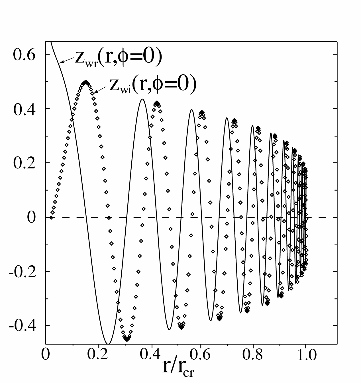
Figure 24: From left to right: (1) Profiles of the real and imaginary parts of the displacement of the disc $z_{w}(r,\phi=0)$ for the ‘inner warp’, $r/r_{cr}<1$, assuming $c_{s}/(r\Omega)=0.05$. (2) Vertical displacement of the disc $z_{w}(r,\phi)$ for the ‘inner warp’, $r/r_{cr}<1$, assuming $c_{s}/(r\Omega)=0.05$. Here, white = negative and red = positive. (3) Real and imaginary parts of the disc displacement $z_{w}$ for the ‘outer warp’ from equation A1. (4) Vertical displacement of the disc $z_{w}(r,\phi)$ for the ‘outer warp’ for $1<r/r_{cr}<2.5$ assuming $c_{s}/(r\Omega)=0.05$.

The left two panels in Fig. 3 show an expanded view of the warp shown in Fig. 2, both in side and face projections. The right two panels show the locations of resonances calculated theoretically for a thin Keplerian disc (see Table 3 and Appendix A). One can see that the amplitude of the bending wave increases at the corotation radius, stays high at the Outer Vertical Resonance (OVR) and gradually decreases at larger radii, where it forms a trailing spiral wave. According to the theory (e.g., Kato et al. 1998; Zhang & Lai 2006, see Sec. A.1 of the Appendix A) a bending wave is expected to have its maximum amplitude at and around vertical resonance (see Fig. 24 of the Appendix, 3rd panel from the left). Fig. 3 shows that in our simulations, the warp has its maximum amplitude between CR and OVR.

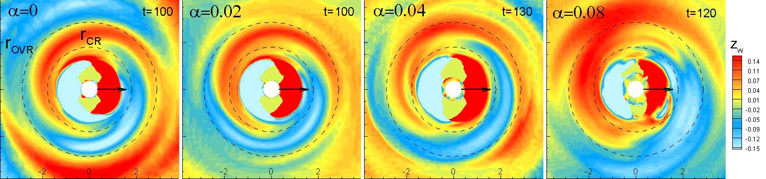
Figure 11: Warps observed in simulations where the viscosity parameter $\alpha$ varies from $\alpha=0.0$ to $\alpha=0.08$ (models FW$\alpha$0.00 - FW$\alpha$0.08 ).

The shape of the bending wave observed in our simulations is similar to that derived from the theoretical analysis (see right panel of Fig. 24 in Sec. A.1). The right-hand panel shows the distribution of density waves, and the locations of the resonances.

According to the theory (e.g., Zhang & Lai 2006), one-armed ($m=1$) in-plane ($n=0$) density waves can propagate to the exterior of OLR, while two-armed ($m=2$) waves can propagate to the exterior of OLR and to the interior of ILR. In our case, there are clear, two-armed density waves which propagate at $r>r_{\rm OLR}$, which is in agreement with the theory. The ILR is located inside the magnetosphere and therefore, there is no disc at $r<r_{\rm ILR}$. It is possible that these density waves are excited directly by the magnetic forcing on the inner parts of the disc. Alternatively, the magnetic force may excite predominantly bending waves, which in turn compress matter and generate density waves. A one-to-one comparison between bending and density waves shows some similarity in the pattern between them, so that this is a possibility.

We apply the spectral analysis described in Sec. 2.3.2 to this model (FW$\mu$1.5). The top left panel of Fig. 4 shows PSD for the one-armed ($m=1$) bending ($n=1$) waves. It can be seen that PSD has a clear feature corresponding to a warp, which rotates rigidly with the angular velocity of the star. This feature starts at the corotation radius and extends outward to a distance of $r\approx 2.7r_{m}$. There are also lower-frequency bending waves, which are at frequencies above or below Keplerian. The higher-frequency waves may represent a coupling between free bending oscillations which have approximately the local Keplerian velocity and bending waves excited by the star. Waves of the lowest frequency may represent a coupling between Keplerian frequency and the frequency of free, bending oscillations of the disc. Analysis of the two-armed ($m=2$) bending waves shows that these waves are much weaker with a PSD negligibly small compared with the one-armed bending wave.

We also calculated the PSD for one-armed and two-armed density waves, and observed that the PSD of a two-armed wave is much stronger. Fig. 4 (bottom right panel) shows that for radii $r_{\rm OLR}<r<5$, there is a feature with angular frequency $\omega\approx 0.25-0.3$ which corresponds to the density waves observed in Fig. 2 (bottom panels). This frequency corresponds to the frequency of both waves. In addition, PSD is high for several frequencies at $r<r_{\rm CR}$. One of these frequencies (the highest) may correspond to trapped waves (e.g., Lovelace et al. 2009)(see Sec. 3.3.2). These waves appear where the angular velocity of the disc decreases to match the angular velocity of the star for the case where the magnetosphere rotates slower than the inner disc. In this model, the corotation radius is only slightly larger than the magnetospheric radius. Nevertheless, there is a maximum in the angular velocity distribution (solid red line in Fig. 4) where trapped waves can form.

Fig. 4 (right bottom panel) shows a candidate trapped wave, which is located interior to the peak in angular velocity distribution at $r\approx 1.5$ and its angular velocity $\omega=0.9$ which is slightly higher than $2\Omega_{*}\approx 0.83$. The non-Keplerian dependencies of $\kappa$ and $\Omega$ are fully accounted for in Lovelace et al. (2009).

There is another density wave at about the same distance, $r\approx 1.5-1.6$ but at a lower frequency, $\omega\approx 0.7-0.8$. This may be a wave excited by magnetic force at the disc-magnetosphere boundary, but it weakens at the corotation radius. There is also a wave at frequency $2\Omega_{*}$ with smaller PSD. This wave may be excited by the warp in the disc. One-armed density waves have negligibly small PSD (right top panel).

It is interesting to note that the PSD for density waves is very different from that for bending waves. This supports the first hypothesis discussed above that bending and density waves are excited independently by the tilted magnetosphere.

3.2.2 Formation of fast warp and other waves in the case of a smaller magnetosphere (FW$\mu$0.5 - base model)

We calculated another similar case, but for a star with a smaller magnetic moment, $\tilde{\mu}=0.5$. In this case the disc is truncated at a smaller radius, $r_{m}\approx 1.2$. We took a smaller corotation radius, $r_{cr}=1.5$, in order to have $r_{m}\approx r_{cr}$ as in model FW$\mu$1.5 (here, we obtain slightly larger value, $r_{cr}/r_{m}\approx 1.25$ compared with the model FW$\mu$1.5, where $r_{cr}/r_{m}\approx 1.15$). We observed that this case is similar to model FW$\mu$1.5, however all scales are smaller because of the smaller size of the magnetosphere, which excites the waves.

Fig. 5 (top panels) show a 3D view of bending waves and the inner warp. The middle panels show that a bending wave forms at the corotation radius and propagates outward. The inner part of the bending wave (a warp) is located at the same position indicating that the warp corotates with the star. The bottom panels show the formation of two-armed density waves, similar to model FW$\mu$1.5, but at smaller scale.

Fig. 6 (left two panels) shows expanded views of the warp in two projections. The two right panels show the positions of bending and density waves relative to resonances. One can see that the warp part of the bending wave is located between the corotation and the vertical resonances, with maximum amplitude at the vertical resonance. The right-hand panel shows that density waves are excited at the Lindblad resonance but are damped rapidly at $r\approx 3.4$, which approximately corresponds to the radial extent of the warp. In addition, one can see density enhancements between the closed magnetosphere and the corotation radius. These are trapped density waves.

Fig. 7 (left panel) shows that in the PSD plot the main feature corresponds to the warp which rotates with the angular velocity of the star and spreads out to $r\approx 3$, which is $2.5$ radii of closed magnetosphere.

The right-hand panel of Fig. 7 shows that the two-armed outer density wave is located at $r_{\rm OLR}<r\lesssim 4$. The angular frequency (for both waves) is $\omega\approx 0.4$. PSD also shows a two-armed trapped density wave with angular frequency $\omega\approx 1.14$ which is located at the inner disc, with $r\approx 1.15$. The frequency of this wave is located below the maximum in the disc angular velocity distribution.

Thus, the warp and other features in model FW$\mu$0.5 are similar to those of model FW$\mu$1.5, which has a larger magnetosphere. In both cases, the warp forms near the magnetosphere and corotates with the star. The warp extends out to $r\approx(2.5-2.7)r_{m}$ and rotates rigidly in this region. Below, we use a model with a larger magnetosphere, FW$\mu$1.5, to determine the amplitude of the warp. In all other models, we use model FW$\mu$0.5 as a base case. For this model, the simulation runs are not as long, and we can investigate the model at a number of different parameters (see Table 2).

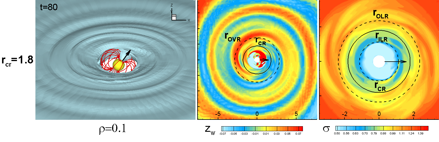
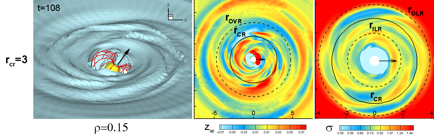
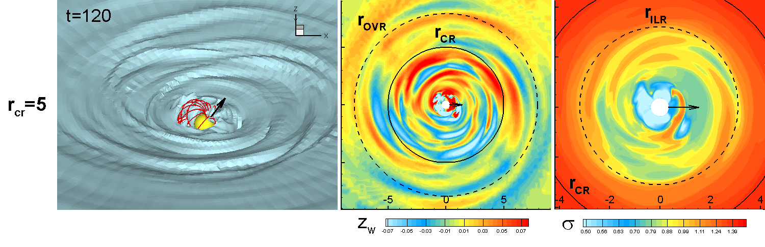
Figure 12: Waves observed in models with large simulation region ($R_{out}=20.2=57.7R_{*}$) at different corotation radii. From top to bottom: models LRcor1.8, LRcor3, and LRcor5. Left panels: 3D view at one of the density levels ($\rho$); Middle panels: bending waves ($z_{w}-$distribution); Right panels: density waves ($\sigma-$distribution).

3.2.3 Amplitude of the warp

It is important to know the amplitude of the warp. A large-amplitude warp can block or diminish the light from a star. In fact, this mechanism of light-blocking by a warped inner disc has been proposed as an explanations for dips in the light-curves observed in some T Tauri stars (Bouvier et al., 2003, 2007b; Alencar et al., 2010). Clearly, the warp amplitude needs to be sufficiently large to produce the observed dips.

Figures 2 and 5 (middle panels) show the amplitude of the warp, $z_{w}$ (the position of the center of mass of the disc relative to the equatorial plane). Warp amplitude is the largest, reaching $z_{w}\approx 0.2$, in model FW$\mu$1.5. Taking into account the distance of this maximum to the star, $r\approx 2$, we obtain the ratio: $z_{w}/r\approx 0.1$. In the model with a smaller magnetosphere, FW$\mu$0.5, we find $z_{w}\approx 0.1-0.15$, and the ratio $z_{w}/r\approx 0.05$. These numbers are in agreement with the theoretical analysis of warped discs by Terquem & Papaloizou (2000), who concluded that the amplitude of the warp is expected to be $5-10\%$. However, they considered the case of a very thin disc.

In a realistic situation, the disc has a finite thickness, and the height of the warp $h_{w}$ that can obscure light from the star can be larger than the deviation of the center of mass from the equatorial plane, $z_{w}$. The density in the disc decreases with height, and the height of the warp also depends on the chosen density level, $h_{w}=h_{w}(\rho)$.

To determine the height of the warp from our simulations, we chose model FW$\mu$1.5, which has a larger magnetosphere. Fig. 8 (bottom panel) shows a view of the magnetosphere and the inner warp, while the top panel shows a slice of the density distribution in the $xz$ plane, which crosses the warp (note that the slice does not go through the maximum amplitude of the warp, which is at about $30^{\circ}-40^{\circ}$ clockwise from the $xz-$plane).

The top panel shows that the height of the warp depends on the chosen density level: the lower the density level, the higher the warp. In the figures, we chose a set of density levels. One can see that at the highest density levels (red color), the warp amplitude is not very large, while at the lowest shown density level (dark blue) the warp rises up to $30\%$ of the distance to the star ($h_{w}/r=0.3$) and can be significant in blocking the light at different inclination angles of observer. The warp amplitude is even larger at even lower density levels. However, for an analysis of light obscuration by the warp, it is important to know the opacity at different density levels in each particular case. We note that the stellar light can also be obscured by the funnel streams, which are located closer to the star than the warp, and can provide an even larger efficient height of the obscuring material, $h_{w}/r>0.3$.

The relative amplitude $z_{w}/h_{w}$ and the height of the warp, $h_{w}/r$, depend on the force which magnetosphere applies to the inner disc. It is expected that both values should increase with the size of the magnetosphere, that is with $\tilde{\mu}$. Comparison of amplitudes done in previous sections, shows that the ratio $z_{w}/r$ is indeed twice as large in case of larger magnetosphere, $\tilde{\mu}=1.5$, than in small magnetosphere, ($\tilde{\mu}=0.5$).

It may also depend on the temperature of the inner disc and its thickness. Fig. 8 shows that the accretion disc is thin, compared with the height of the warp and hence the magnetic force is the main one which determines the height of the warp in this model.

We observed from our simulations that the ratios $z_{w}/r$ and $h_{w}/r$ are larger in model FW$\mu$1.5 (with a larger magnetosphere, $r_{m}\approx 4.7R_{*}$), compared with model FW$\mu$0.5 (where the magnetospheric radius is smaller, $r_{m}\approx 3.3R_{*}$). This is because a larger magnetosphere applies stronger magnetic force to the disc (which has the same properties in these two models). We suggest, that an even stronger warp can be expected in the cases of an even larger magnetosphere. It is expected that in many CTTSs, the disc can be truncated at larger distances (e.g., $r_{m}\approx(7-8)R_{*}$ in AA Tau star, Donati 2011). Special investigations are needed to understand whether the amplitude and height of the warp will increase or decrease with a further increase of $r_{m}$.

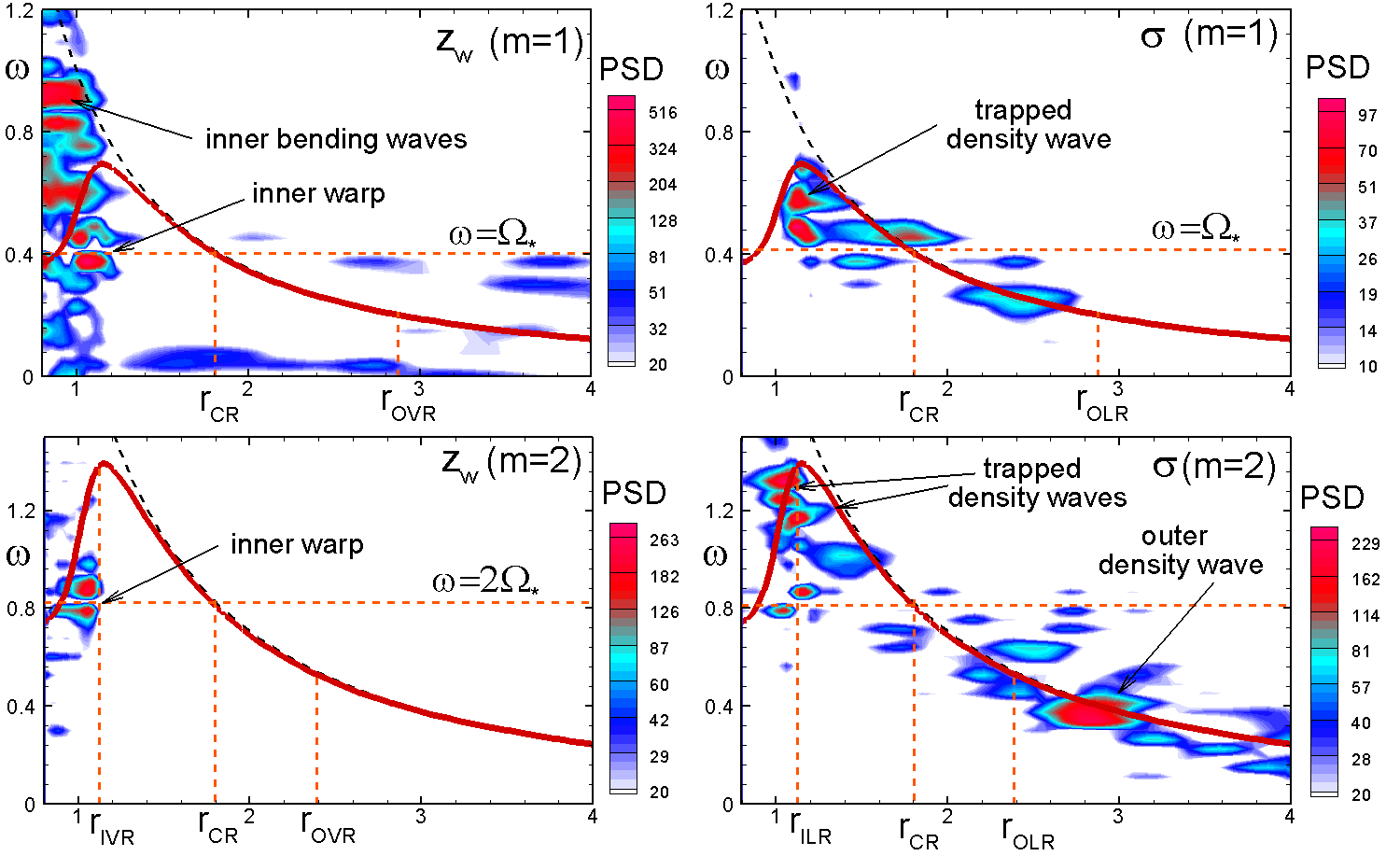
Figure 13: PSD of oscillations (color background) for waves in model LRcor1.8 (large region, $r_{cr}=1.8$). The solid red lines show the angular velocity distribution in the disc

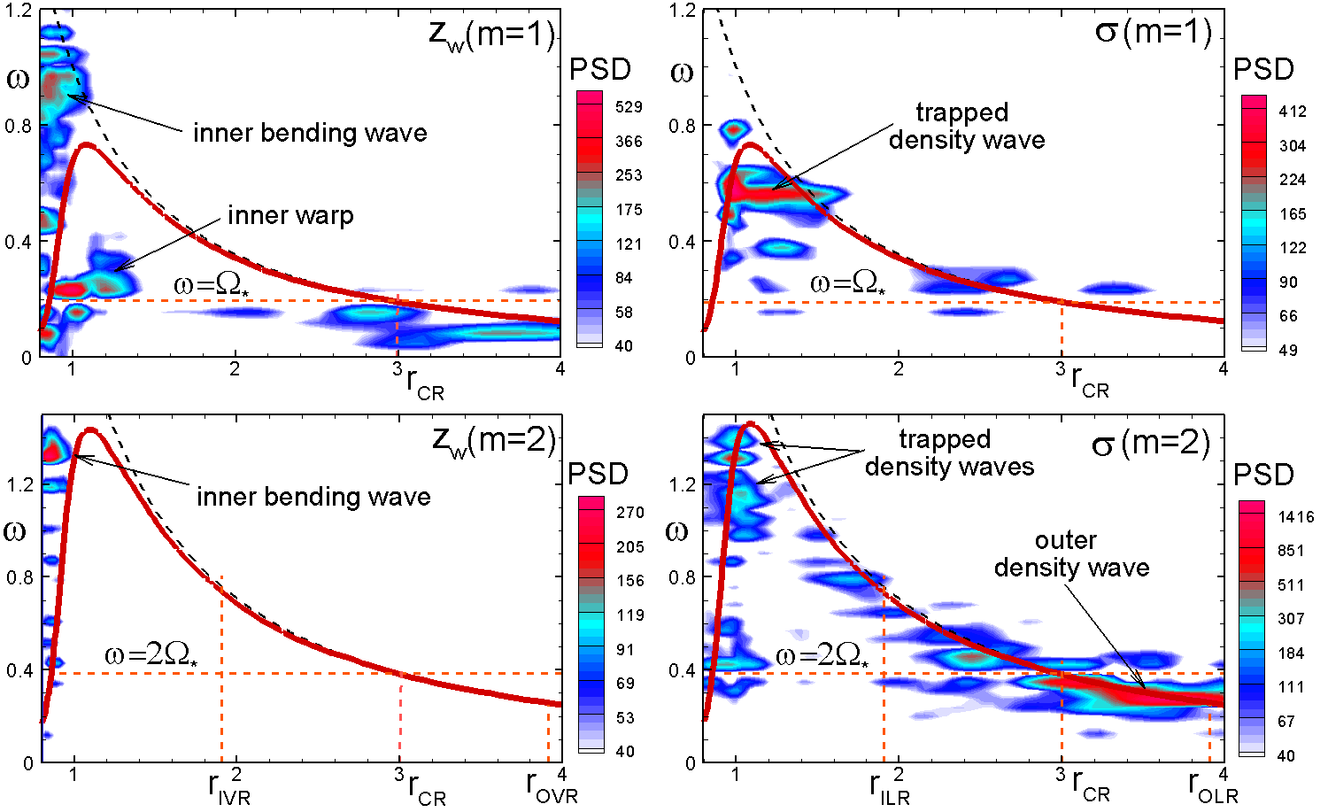
Figure 14: Same as in Fig. 13, but for model LRcor3 (large region, $r_{cr}=3$).

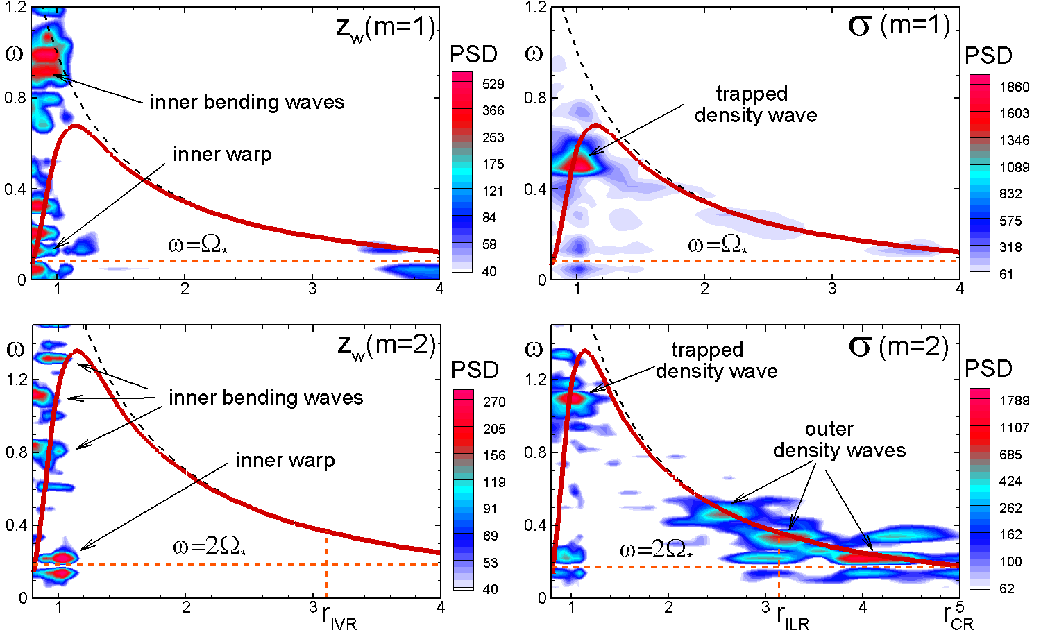
Figure 15: Same as in Fig. 13, but for model LRcor5 (large region, $r_{cr}=5$).

3.2.4 Warps in the cases of different tilts of the dipole, $\theta$

Here, we investigate the dependence of the warp amplitude $z_{w}$ on the misalignment angle of the dipole moment relative to the star’s spin axis, $\theta$. For this reason, we performed a series of simulations at different $\theta$ values, from $\theta=5^{\circ}$ up to $\theta=90^{\circ}$ (models FW$\theta$5, FW$\theta$15, FW$\theta$45, FW$\theta$60, and FW$\theta$90). We take as a base model FW$\mu$0.5, where $\theta=30^{\circ}$.

Fig. 9 shows the results for cases of relatively small tilts of the dipole: $\theta=5^{\circ},15^{\circ}$, and $30^{\circ}$. The top panels show slices of density distribution in the $xz-$plane and sample field lines. One can see that the inner disc is thicker in models with smaller $\theta$. The densest part of the disc (red color) shows bending waves. The middle panels show a 3D view of the bending waves at one density level. One can see that waves are excited in all three models. The bottom panels show the amplitude of the warp, $z_{w}$. A warp forms in all three cases, with the maximum at the vertical resonance (outer dashed circle). From these plots, we find the values $z_{w}/r\approx 0.025$, $0.045$, and $0.05$ in models with $\theta=5^{\circ},15^{\circ}$, and $30^{\circ}$, respectively.

The height of the warp, $h_{w}$ is larger than $z_{w}$. Top panels of Fig. 9 show that at small values of $\theta$ ($5^{\circ}$ and $15^{\circ}$), the magnetosphere is an obstacle for the disc matter, and matter accumulates at the disc-magnetosphere boundary, thus making the disc thicker. Such an inner disc can absorb stellar light, thus providing $h_{w}/r\approx 0.3$. At $\theta=30^{\circ}$, the amplitude of the warp $z_{w}$ is larger than in the other two cases. However, the height of the inner disc is smaller.

The bottom panels of Fig. 9 show that in cases where $\theta=5^{\circ}$ and $15^{\circ}$, some matter accretes to the star through a Rayleigh-Taylor instability (e.g., Romanova et al. 2008; Kulkarni & Romanova 2008). However, this does not prevent excitation of bending waves, because these phenomena occur at different radii: unstable accretion occurs at the inner regions of the disc, while bending waves are excited at somewhat larger distances by the external parts of the magnetosphere.

Fig. 10 shows the excitation of bending waves around stars with larger misalignment angles: $\theta=45^{\circ},60^{\circ}$ and $90^{\circ}$. Top two panels show that bending waves are excited in all of these cases. However, the bottom panel shows that a high-amplitude warp forms only when $\theta=45^{\circ}$ and $60^{\circ}$ (with ratios $z_{w}/r=0.04$ and $z_{w}/r=0.03$, respectively), while in the case of $\theta=90^{\circ}$, where the magnetosphere cannot provide strong perturbations in the $z-$direction, the ratio $z_{w}/r$ is about $10-20$ times smaller than that in the other two cases.

3.2.5 Influence of viscosity on the warps

In our code an $\alpha-$type viscosity is incorporated into the disc. Viscosity is thus regulated by the parameter $\alpha$ (see Shakura & Sunyaev 1973). All of the above-mentioned simulations were performed for a relatively small viscosity, $\alpha=0.02$. Here, we show the results of our simulations for the base model FW$\mu$0.5 but with different viscosities: $\alpha=0,0.04,0.06$ and $0.08$.

Fig. 11 shows bending waves for different $\alpha$ values. One can see that in all of the cases a warp forms, and is located at approximately the same place, with a maximum amplitude between corotation and vertical resonances, or at the vertical resonance.

The possible influence of viscosity on the evolution of warped discs has been investigated earlier (papaloizou83; Papaloizou & Lin 1995; Terquem & Papaloizou 2000; Ogilvie 2006). Papaloizou & Lin (1995) considered the formation of warps in viscous $\alpha-$type discs, which have a vertical scale height $h(r)$, and concluded that to a first approximation, the warp satisfies a wave-type equation if $\alpha\lesssim h/r$. In the opposite case, if $\alpha\gtrsim h/r$, the warp satisfies a diffusion-type equation (papaloizou83).

In our simulations, the ratio $h/r\approx 0.1$. Therefore, we expect non-diffusive, wave-like behavior for $\alpha$ values smaller than $\alpha=0.1$. Hence, our range of parameters, $\alpha\leq 0.08$, satisfies this condition. Simulations show that amplitudes of warps and bending waves are similar in all cases. This is somewhat unexpected result, because according to the theory, even in the wave regime, the viscosity should damp the waves (e.g., Ogilvie 1999; Terquem & Papaloizou 2000). We do not see such damping. We suggest that this issue requires further study and possibly a larger set of numerical simulations.

3.3 Waves in cases where the magnetosphere rotates slower than the inner disc, $r_{m}<r_{cr}$

In the above section we investigated cases where the magnetosphere and the inner disc rotate approximately with the same angular velocity, which corresponds to the rotational equilibrium state (e.g., Long et al. 2005). We observed that the main feature is a warp corotating with the star. However, the situation is different when the magnetosphere rotates much slower than the inner disc, that is, when the corotation radius $r_{cr}$ is much larger than the magnetospheric radius, $r_{m}$. Such a situation may arise during periods of enhanced mass accretion, when the disc compresses the magnetosphere and the magnetospheric radius $r_{m}$ decreases. Alternatively, the dipole component of the magnetic field of a young star may decrease due to internal dynamo processes (e.g., Donati 2011). As a result, the magnetospheric radius $r_{m}$ will decrease, providing the condition $r_{m}<r_{cr}$.

If the magnetosphere rotates slower than the inner disc, then it applies force to the inner disc, but with relatively low frequency of the star’s rotation, $\Omega_{*}$. This will excite bending and density waves with the frequency of the star. On the other hand, the matter of the inner disc has a higher angular velocity. It interacts with the slowly-rotating magnetosphere, which serves as a non-axisymmetric obstacle for the disc matter flow. It exerts a non-axisymmetric force on the inner parts of the disc, thus exciting higher-frequency waves (both density and bending waves). Thus, a complex pattern of waves is expected in this case. In addition, we observed that a slowly-rotating star excites global bending oscillations of the whole disc if the size of the simulation region (that is, the size of the disc) is not very large. In the case of a large simulation region, these waves are also excited, but their frequency is very low and they are excited slowly compared with the overall time of simulations. This is why we initially consider the case of a relatively large simulation region, where these low-frequency waves can be neglected (see Sec. 3.3.1). Next, we investigate the cases of smaller simulation regions, where global disc oscillations develop and couple with other frequency modes (see Sec. 3.4).

3.3.1 Investigation of waves in a large disc

Here, we investigate the waves excited in a relatively large simulation region, with radius $R_{max}=20.2\approx 57.7R_{*}$. This region is 1.7 times larger than that used in Sec. 3.2. We observe that the very low-frequency global mode of disc oscillations develops slowly, and we are able to investigate higher-frequency oscillations at the “background” of this slowly-growing mode.

We use a model with parameters corresponding to our base model FW$\mu$0.5, but take a larger simulation region and a larger corotation radius: $r_{cr}=1.8,3$ and $5$ (models LRcor1.8, LRcor3, and LRcor5). The magnetospheric radius $r_{m}\approx 1.15$ is located at the same place as in model FW$\mu$0.5. Hence, the new models correspond to stars with slower rotation. The simulations show that matter in the rapidly-rotating inner disc interacts with the slowly-rotating tilted magnetosphere of the star, so that different types of waves are excited and propagate to larger distances.

Fig. 12 (top row) shows the results of our simulations for model LRcor1.8, where the corotation radius is $r_{cr}=1.8$, and the star rotates relatively rapidly compared with the other two cases. The left and middle panels show that a bending wave is excited at the disc-magnetosphere boundary and propagates outward, forming a spiral wave. The amplitude is enhanced at the outer vertical resonance, $r=r_{\rm OVR}$ (see Table 3), and this enhancement has a position similar to that of the warp in the base case (FW$\mu$0.5), where the wave corotates with the star. Here, however, instead of corotation, we observe a tendency to corotate, where a wave rotates with the frequency of the star during only a part of the rotational phase, then it slows down, but soon after, another similar wave appears and corotates with the star, and so on. The right panel shows surface density distribution, $\sigma$. One can see that different waves form at different radii from the magnetosphere, including a two-armed density wave, which forms at the outer Lindblad resonance.

Next, we show the results for model LRcor3, where the corotation radius is larger, $r_{cr}=3$. Fig. 12 (middle row)) shows that bending waves are less ordered inside the corotation radius compared with model LRcor1.8. They look like parts of a tightly wound spiral wave extending out to the corotation radius. At larger distances, a new bending wave is formed, and it is more ordered and not as tightly wound. This observation is in agreement with the theoretical prediction, where a tightly wound spiral wave is expected at $r<r_{cr}$ (see the left two panels of Fig. 24 in Appendix A), and a much less tightly wound spiral is expected at $r>r_{cr}$ (see Fig. 24, right panels). The right-hand panel of Fig. 12 (middle row) shows that different density waves formed between the inner radius of the disc and the OLR radius.

Next, we show the results for model LRcor5, where the corotation radius is even larger, $r_{cr}=5$. Fig. 12 (bottom row) shows that bending waves are not ordered and have a rippled structure, as in the $r_{cr}=3$ case. The middle panel shows that bending waves are not ordered, but one can track a tightly wound spiral wave inside the corotation radius (in agreement with Fig. 24 of Appendix A). A more ordered, but less tightly wound spiral wave starts at $r\approx r_{cr}$ and becomes yet more ordered at the OVR. The right-hand panel shows density waves. One can see that different density waves propagate at $r<r_{ILR}$. There are waves at larger distances, but they are not seen at the chosen density levels.

The PSD shows interesting sets of bending and density waves in these three models (see Figures 13, 14 and 15). The PSD confirms that there is no large-scale warp at the stellar frequency, which is different from models FW$\mu$0.5 and FW$\mu$1.5 (see Sec. 3.2). Instead, only a small-scale bending wave is excited at the stellar frequency or at twice this value (see left panels of the figures for $m=1$ and $2$). This wave is only present at the inner region of the disc, close to the region where matter lifted to the funnel flow, and may therefore reflect this lifting. For the three models considered, the angular frequency of the wave is low. For example, in the case of a one-armed wave ($m=1$), $\omega\approx 0.41,0.19$ and $0.09$ for models LRcor1.8, LRcor3 and LRcor5, respectively.

There are also high-frequency bending waves associated with interaction of the rapidly-rotating matter of the inner disc with the non-axisymmetric magnetosphere. The angular frequency of these waves, $\omega\approx 0.8-1$, approximately corresponds to Keplerian velocity of the inner disc. Also, there are bending waves of intermediate frequency. All of these waves are located at the inner edge of the disc, $0.8<r<1.2$ where matter has already been lifted, or has started lifting to the funnel flow.

Lower-frequency bending waves excited by the slowly-rotating star propagate from the disc-magnetosphere boundary to large distances, and we often see an enhanced PSD at the stellar frequency, and at different distances from the star. The PSD can be further enhanced at the corotation radius, as we can see in Fig. 14 (top left panel). The stellar-frequency mode is also seen in other models, but at lower values of PSD.

The density waves show a variety of frequencies (see right-hand panels of figures 13, 14 and 15). At low frequencies, we observe enhanced PSD at radii $\sim 3-4$, which often correlate with a position of different resonance (e.g., in model LRcor1.8 with OLR, in model LRcor3 with CR and OLR, in model LRcor5 - with ILR). Plots of the surface density distribution $\sigma$ for these models (see Fig. 12) show that in all these models, the density waves have higher amplitudes at the distances of $r\lesssim 4$, where the influence of the rotating magnetosphere is stronger.

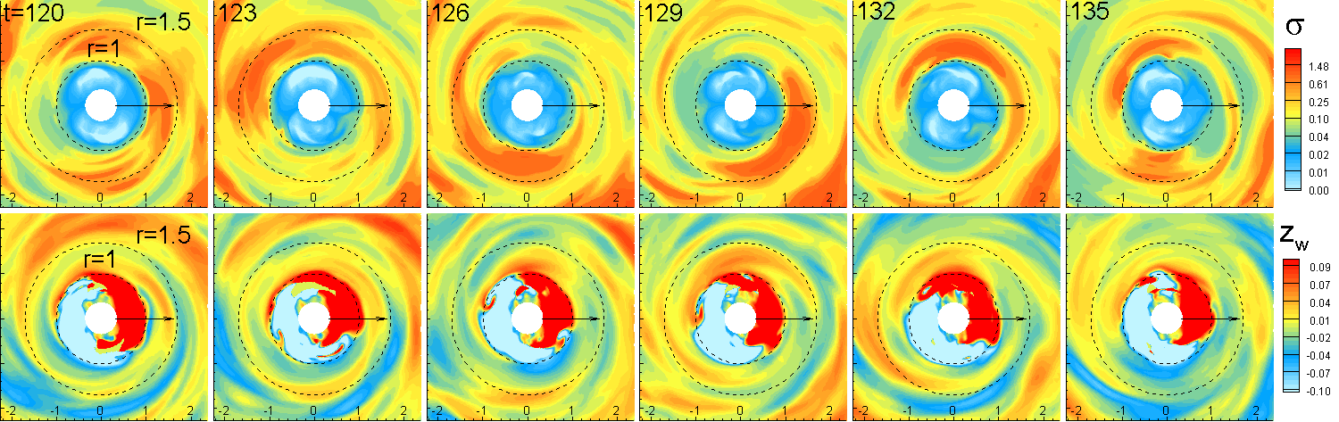
Figure 16: Evolution of density (top panels) and bending (bottom panels) waves at the inner disc in model LRcor3 (large region, $r_{cr}=3$). Dashed circles show radii $r=1$ and $r=1.5$ (for scale).

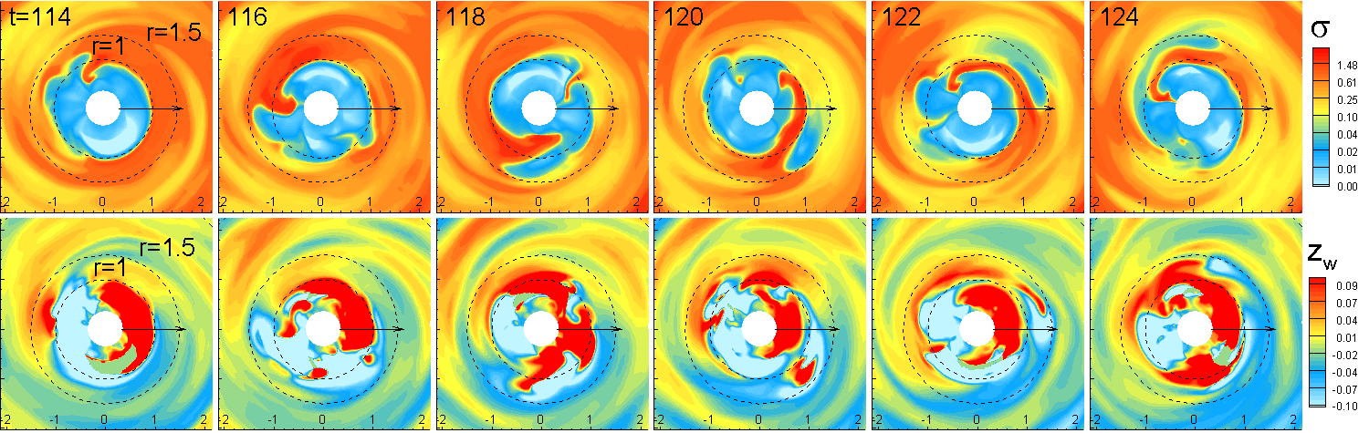
Figure 17: Same as in Fig. 16, but for model LRcor5 (large region, $r_{cr}=5$).

3.3.2 Waves in the inner disc: trapped density waves

At high frequencies, the PSD of density waves is often enhanced at radii corresponding to the peak in the angular velocity distribution, and the frequencies of these waves are usually somewhat lower than the peak frequency (see Fig. 13, 14 and 15, where the solid red lines show the angular velocity distribution in the disc). We suggest that these are trapped density waves, which are expected in cases where the angular velocity distribution in the disc has a maximum (Lovelace & Romanova, 2007; Lovelace et al., 2009). In our models, the maximum in the angular velocity as a function of $r$ occurs because the star rotates slower than the inner disc. The region where the angular velocity decreases gives rise to the possibility of radially trapped unstable Rossby waves with azimuthal mode numbers $m\geq 1$ and radial width $\Delta r/r\ll 1$ (Lovelace et al. 2009). The theory of trapped waves is summarized in Appendix B. It is important that the Rossby waves have density variations as well as temperature variations, and hence they appear in our simulations and analysis as density waves. Here, we analyze trapped waves in one of our models (LRcor3), where these waves are clearly observed. Fig. 14 shows a high-frequency ($\omega\approx 0.57$), one-armed ($m=1$) wave, which is located below the maximum in $\omega$ at radii $1<r<1.5$. To check this wave we also plot the surface density distribution at the inner disc for different times and clearly see that there is a one-armed wave located approximately between radii 1 and 1.5 (see Fig. 16). We believe that this is a trapped density wave. According to the theory (Lovelace et al. 2009), trapped waves have a tendency to be within the maximum in the $\omega$ distribution. We can see that in model LRcor3, the maximum of the PSD for $m=1$ is located in the left part of the $\omega-$curve, while for model LRcor5, the trapped wave is located below the maximum of $\omega$ for both the $m=1$ and $m=2$ modes.

The bottom panels of Fig. 16 show bending waves for the same moments in time. A small inner warp forms at $1<r<1.5$, but rotates with the angular velocity of the star. This small warp is also seen in Fig. 14 (top left panel). The PSD also shows the presence of a high-frequency, ($\omega\approx 1$), bending wave at $r<1$ (top left panel). This feature probably corresponds to a small funnel or tongue, which forms due to the magnetic Rayleigh-Taylor (RT) instability at the disc-magnetosphere boundary.

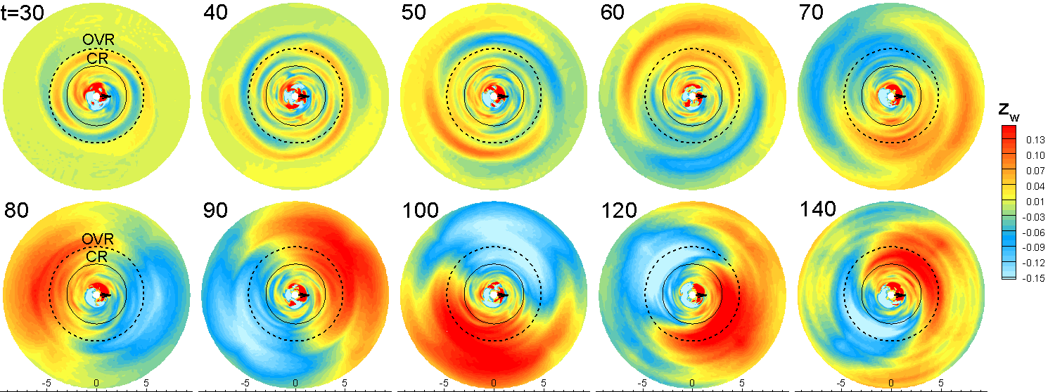
Figure 18: The sequence of panels shows how a bending wave near the star excites a global oscillation of the whole disc. Simulations are performed in a relatively small region, $R_{out}=9.4=26.9R_{*}$, for demonstration (model SRcor3).

3.3.3 Accretion through instabilities: density and bending waves

At the disc-magnetosphere boundary, matter can penetrate through the magnetosphere due to the magnetic Rayleigh-Taylor (RT) instability (e.g., Arons & Lea 1976; Spruit & Taam 1990; Kaisig et al. 1992). A necessary condition for the instability is that the gravitational acceleration towards the star be larger than the centrifugal acceleration. Additional factors are also important, such as the gradient of the angular velocity in the inner disc and the gradient of the surface density (e.g., Spruit et al. 1995). Global numerical simulations of accretion onto a star with a tilted dipole magnetic field show that accretion may be in the stable or unstable regimes (see Romanova et al. 2008; Kulkarni & Romanova 2008, 2009; Bachetti et al. 2010). In the stable regime, matter accretes in ordered funnel streams, which corotate with the star. In the unstable regime, matter accretes through unstable temporary funnels or tongues, which carry the angular momentum of the inner disc, and can rotate faster than the inner disc matter. The simulations show that the criterion for the onset of the RT instability is close to that derived by Spruit et al. (1995). In addition, the boundary between stable and unstable regimes depends on the tilt of the magnetosphere and on the simulation grid . At larger tilt angles, more matter accretes in stable funnel streams.

In our models with $r_{cr}=3$ and $5$, a star rotates slowly relative to the inner disc, and therefore the instability is favored. On the other hand, the tilt of the dipole is relatively large ($\theta=30^{\circ}$), and this favors accretion through funnel streams. This is why in the case of $r_{cr}=3$, where the star rotates relatively slowly, we see only a weak instability. To demonstrate accretion through instabilities, we take an even slower rotating star, where $r_{cr}=5$ (model LRcor5) and accretion through the RT instability is very clear. The top panels of Fig. 17 show that the instability leads to the formation of one main “tongue”, which rotates with the angular frequency $\omega\approx 0.5$. This unstable tongue is associated with the main one-armed trapped density wave that forms in the inner disc. The frequency of this trapped wave is clearly seen in Fig. 15 (top right panel). The PSD also shows the presence of a second harmonic ($m=2$) with $\omega\approx 1.1$ at radius $r\approx 1$ (see bottom right panel of Fig. 15). This wave is barely seen in the surface density plots in Fig. 17, but is clearly seen in the PSD.

The bottom panels of Fig. 17 show that the instability is also seen in the bending waves that form at the inner edge of the disc. The two-armed bending wave (bottom left panel of Fig. 15) also has a mode $\omega\approx 1.15$ at $r<1$, which is close to the mode $\omega=1.1$ of the $m=2$ trapped density wave. Here, we have an example of how a trapped density wave generates unstable tongues at smaller radii. Another possible explanation is that both waves indicate accretion through instabilities.

Fig. 15 (top left panel) shows the presence of a high-frequency ($\omega\approx 0.9-1.1$), one-armed ($m=1$) bending wave at $r<1$. A similar mode is observed in two other models (LRcor1.8, LRcor3). This mode is probably connected with the rotation of unstable funnel streams at the inner edge of the disc. The frequency of the mode is higher than that of the disc (solid red line). We suggest that this mode may reflect the rotation of temporary unstable funnel streams, which are lifted above the magnetosphere, and therefore do not experience magnetic braking (as matter in the disc does), and hence can rotate with a nearly Keplerian velocity. We call these waves inner bending waves.

3.4 Waves in a smaller simulation region: global disc oscillations and slowly-rotating warps

In sections 3.3.1-3.3.3, we considered the case of a relatively large region, where free bending oscillations in the disc develop slowly. In this section, we consider a smaller simulation region, in which we observe that these oscillations develop more rapidly.

First, we demonstrate the excitation of free bending oscillations in the disc of a very small size, $R_{out}=9.4=26.9R_{*}$ (model SRcor3). The simulations show that initially, waves are excited at the disc-magnetosphere boundary (see top panels of Fig. 18). Later, at $t\approx 70-100$, global bending oscillations of the disc develop. However, at $t>100$, the maximum of the bending wave amplitude moves to the region between the OVR and the CR resonances (see Fig. 18). This feature is similar to the warps in cases of rapidly-rotating stars (see Sec. 3.2). However, this new warp rotates slower than the star.

Next, we investigate the waves in the intermediate-sized simulation region, $R_{out}=12.1=34.5R_{*}$, where free bending oscillations in the disc develop sufficiently fast in particular in cases of slowly-rotating stars). We consider two models with corotation radii $r_{cr}=1.8$ and $3$ (models SWcor1.8 and SWcor3).

In model SWcor1.8, we observed evolution of bending waves similar to that in model SRcor3 (see Fig. 18). As a result of this evolution, a warp forms at radii $r_{\rm CR}<r<r_{\rm OVR}$. This warp rotates slower than the star (see Fig. 19). A closer view of the warped disc (see Fig. 20) shows that a significant part of the inner disc is tilted and involved in this slow rotation.

In the case of an even more slowly-rotating star, $r_{cr}=3$ (model SWcor3), a very slow warp forms at $r>r_{\rm CR}$. Fig. 21 shows the rotation of this warp about the star.

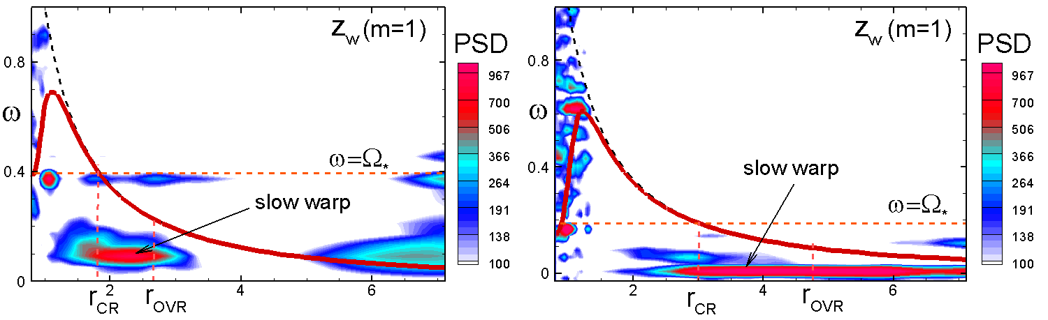
Figure 22: PSD demonstrates low-frequency mode associated with a slow, one-armed ($m=1$) bending wave in models SWcor1.8 (left panel) and SWcor3 (right panel).

Fig. 22 shows the PSD for these two models. One can see that in the case where $r_{cr}=1.8$ case (left panel), the warp rotates with an angular frequency $\omega\approx 0.1$, which is about four times smaller than frequency of the star. The PSD also shows that the main part of the warp is located between the corotation and the vertical resonances. In the case of a slower rotating star ($r_{cr}=3$, right panel), the warp rotates very slowly, with an angular frequency $\omega=0.01-0.02$, though the accuracy of our model is not very high in cases of very low frequencies (because the number of rotations per simulation run is small). One can see that in both cases, the angular frequency of slow warps is much smaller than the local Keplerian frequency. In model SWcor3, the angular frequency of the warp is comparable with the Keplerian frequency at the edge of the simulation region, $\omega_{K}(r\approx 12)\approx 0.024$. However, this is probably just a coincidence. In test simulations with even more slowly-rotating stars ($r_{cr}=5$), a warp forms, and its angular frequency is even lower: $\omega<0.01$. We did not establish how this slow warp forms. Its frequency probably represents a coupling between the frequency of the star and the frequency of global oscillations in the disc.

4 Applications and discussion

The results of our simulations can be applied to various types of stars where the magnetospheric radius is several times larger than the radius of the star , including, for example, classical T Tauri stars, accreting millisecond pulsars that host spun-up neutron stars and some types of cataclysmic variables (such as Dwarf Novae). Possible applications are briefly discussed in sections below.

4.1 Obscuration of light by warped discs in classical T Tauri stars (CTTS) and drifting period

The light curves of classical T Tauri stars (CTTS) display photometric, spectroscopic and polarimetric variations on timescales ranging from a few hours to several weeks (Herbst et al., 2002). Bouvier et al. (1999) studied the variability of AA Tau in great detail and concluded that the photometric variability with a period of $8.2$ days which is comparable to the expected rotation period of the star is due to the occultation of the star by a warp formed in the inner disc (the system is observed almost edge-on). They proposed that this warp is produced by the interaction of the disc with the stellar magnetic dipole tilted with respect to the disc rotational axis. Later, more detailed analysis confirmed the hypothesis of obscuration by the disc (Bouvier et al., 2003, 2007b). Doppler tomography observations of AA Tau show that the dominant component of the field is a $2-3$ kG dipole field that is tilted at $20^{\circ}$ relative to the rotational axis. At this field strength the magnetospheric radius is close to the corotation radius: $r_{m}\approx r_{cr}$ (Donati et al., 2010). Our simulations show that in this situation a large amplitude warp forms and rotates with the frequency of the star, and the AA Tau warp may be similar to that described in model FW$\mu$1.5. An analysis of the warps in cases where the dipole has different tilts (see Sec. 3.2.4) shows that an angle of $\theta\lesssim 20^{\circ}$ is sufficiently large to generate a warp. It is possible that warps are common features in many CTTSs. For example, Alencar et al. (2010) analyzed the photometric variability of CTTSs in the young cluster NGC 2264 using data obtained by the CoRoT satellite and concluded that AA Tau-like light curves are fairly common, and are present in at least  $30-40\%$ of young stars with inner dusty discs (see also Carpenter et al. 2001).

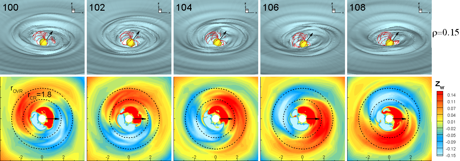
Figure 19: A slowly-rotating warp observed in model SWcor1.8. Top row: 3D views of the warp at different moments in time; Bottom row: center of mass of the disc $z_{w}$, which demonstrates a slowly-rotating warp.

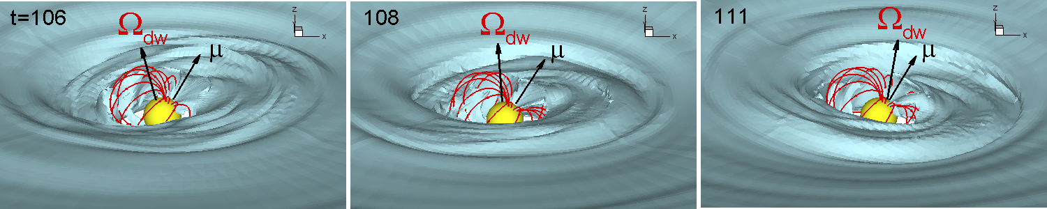
Figure 20: An example of a warp which rotates slower than the star in model SWcor1.8 (simulation region $R_{out}=12.1=34.5R_{*}$). One of the density levels is shown. Vector $\Omega_{dw}$ shows the direction perpendicular to the inner disc warp.

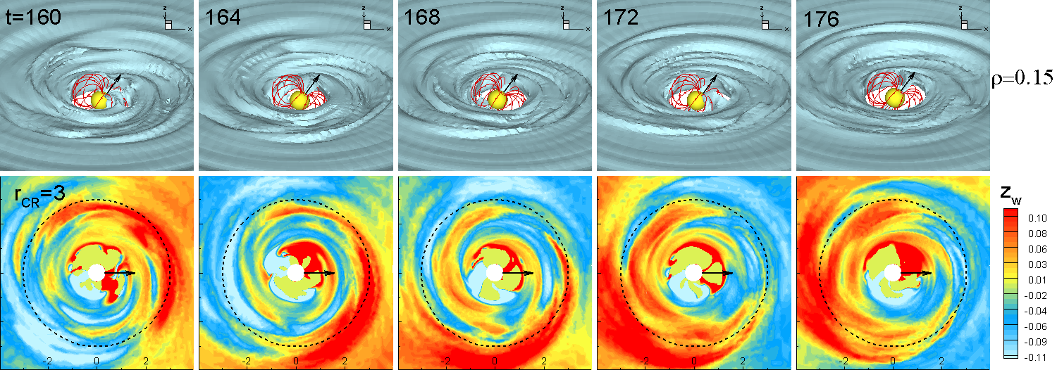
Figure 21: Same as in Fig. 19, but for a slower rotating star, $r_{cr}=3$ (model SWcor3).

Not only fast warps, but also other waves can be generated by the rotating magnetosphere in CTTSs. However, it is difficult to observe these waves in CTTSs: these stars are usually brighter than the inner disc and are strongly variable due to coronal magnetic activity. In addition, observations usually cover not more than a few periods of the star, and it is difficult to extract a possible frequency of the waves from light-curves. One possibility is that the waves generated in the inner disc may influence the formation of magnetospheric streams and their subsequent motion, thereby leaving a trace on the surface of the star in the form of hot spots, which can move faster or slower than the star (Romanova et al., 2004; Bachetti et al., 2010). Observations show that many CTTSs do not have a precise period, but instead a quasi-period, which varies with time around some value (e.g., Rucinski et al. 2008). This quasi-period may be connected with the formation of high-frequency waves, such as trapped density waves. These waves represent regions of enhanced density and therefore probable places where funnel streams may form. The position and frequency of a trapped waves vary with accretion rate. Thus, the angular velocity of hot spots on the surface of the star and the associated quasi-period of the star will also vary.

In a number of situations accretion through the RT instability is possible, where matter accretes in unstable, stochastically-forming tongues (e.g., Romanova et al. 2008; Kulkarni & Romanova 2008). In this case, the light-curve becomes less ordered, and in a strongly unstable case a CTTS may show the absence of a period. It is often the case that the instability is not very strong, and both stochastic and periodic components are expected in the frequency spectrum (Kulkarni & Romanova, 2009). In these cases, trapped density waves can determine the position of unstable tongues. In the case of small magnetospheres, this leads to the formation of two coherent tongues that rotate more rapidly than the star (Romanova & Kulkarni, 2009). Hence, one of the frequencies can be connected with trapped density waves. On the other hand, we often observe in the PSD even higher- frequency oscillations (inner bending waves) that have a nearly Keplerian frequency. Both of these waves may leave an imprint at the surface of CTTSs in the form of moving hot spots. Our simulations show that the coherence of trapped waves is probably higher than that of inner bending waves, and it is more likely that the variable quasi-period of CTTSs is connected with the trapped waves.

4.2 Application to Accreting Millisecond Pulsars

Accreting millisecond pulsars (AMPs) show various types of quasi-periodic oscillations (QPOs), ranging from very high frequencies ($\sim 1,300$ Hz) down to very low frequencies ($\sim 0.1$Hz) (e.g. van der Klis 2006). One of the prominent features in the spectrum of AMPs is a pair of QPO peaks with an upper frequency $\nu_{u}$ and a lower frequency $\nu_{l}$, which move in pairs. The distance between the peaks $\nu_{u}-\nu_{l}$ usually corresponds to either the frequency of the star, $\nu_{*}$, to half this value, $\nu_{*}/2$ (e.g., van der Klis 2000, 2006), or, in some AMPs there is no such correlation (e.g., Méndez et al. 1998; Boutloukos et al. 2006; Belloni et al. 2007; Méndez & Belloni 2007). There are also QPOs with lower frequencies, including hecto-hertz QPOs with a frequency of $\nu_{h}\approx\nu_{u}/4$, as well as low frequency QPOs with a frequency of $\nu_{\rm LF}\approx\nu_{u}/15$. There are also very low-frequency oscillations, $\nu_{LL}\lesssim 1$Hz. Below we discuss possible connections between the waves observed in simulations and some of these frequencies.

4.2.1 High-frequency oscillations in the inner disc

Our simulations show that there are two main types of high-frequency waves: (1) trapped density waves, and (2) inner bending waves. The frequency of the inner bending waves approximately equal to the Keplerian velocity at the disc-magnetosphere boundary. The trapped density wave is located inside the peak in the disc angular velocity distribution, and hence it has lower frequency. We suggest that the trapped waves can be responsible for the lower QPO peak, $\nu_{l}$, and the inner bending wave for the upper QPO peak, $\nu_{u}$.

Variation of the accretion rate leads to variation of the position of the disc-magnetosphere boundary, and therefore the position of both peaks will vary with accretion rate and they will move in pairs. We expect that the quality factor $Q=\nu/\Delta\nu$ of both waves will increase with accretion rate, because when the disc moves closer to the star, the maximum in the angular velocity distribution becomes more pronounced, and the trapped waves become stronger and more coherent. At the same time, accretion through instabilities becomes stronger and more ordered (where one or two tongues become dominant and create a more ordered motion, see Romanova & Kulkarni 2009). This is in agreement with the observations of QPOs, where $Q$ increases with frequency for both upper and lower QPOs (e.g., van der Klis 2000; Barret et al. 2006). The quality factor of lower QPOs starts decreasing at very high frequencies, possibly due to relativistic effects (e.g., Barret et al. 2006).

Waves in the inner disc can influence the magnetospheric flow and can therefore leave imprints on the frequencies of moving spots on the surface of the star. Moving spots on the surface of the star were observed in global 3D simulations of stable magnetospheric accretion (Romanova et al., 2003, 2004) and during accretion through instabilities (e.g., Kulkarni & Romanova 2008). Bachetti et al. (2010) found that rotating spots provide two QPO frequencies: one corresponds to rotating funnel streams and has a lower frequency, while the other corresponds to rotating unstable tongues and has a higher frequency (see also Kulkarni & Romanova 2009). We suggest that these two frequencies represent an imprint of the trapped and inner bending waves, respectively.

We can calculate the difference in frequency between these two high-frequency waves in the disc. For example, in model LRcor3, the frequency of the $m=1$ trapped wave is $\omega_{trap}\approx 0.55$, while the frequency of the inner bending wave is $\omega_{bend}\approx 0.95$ (see top panels in Fig. 14). Then, using Table 1 for millisecond pulsars, we obtain the dimensional frequencies of these waves, $\nu_{l}=247$Hz and $\nu_{u}=427$Hz, and the difference between them, $\Delta\nu=180$Hz. Similarly, in model LRcor5 (see top panels of Fig. 15) we obtain $\omega_{trap}\approx 0.51$ ($\nu_{l}\approx 229$Hz) for the trapped density waves, and two candidate frequencies for the inner bending waves, $\omega_{bend}\approx 0.91$ and $\omega_{bend}\approx 0.99$, which correspond to $\nu_{u}=409$Hz and $\nu_{u}=445$Hz. The difference between the frequencies is $180$Hz and $216$Hz, respectively. This difference is typical for many accreting millisecond pulsars (see bottom panel of fig.1 of Méndez & Belloni 2007).

For case of moving spots, we investigated how frequencies vary with accretion rate and found that the typical difference is $\Delta\nu\approx 200-250$Hz, which is in agreement with the frequency difference for high-frequency waves. This strengthens our hypothesis that the hot spots represent an imprint of the waves in the disc.

We should note that the frequency difference $\Delta\nu$ is approximately the same for stars with $r_{cr}=3$ as for stars with $r_{cr}=5$, and therefore $\Delta\nu$ does not depend on the frequency of the star. This model can explain those AMPs where $\Delta\nu$ does not correlate with the frequency of the star (e.g., Méndez et al. 1998; Boutloukos et al. 2006; Belloni et al. 2007; Méndez & Belloni 2007).

It has been suggested earlier that the high-frequency QPOs may be connected with the rotation of some blobs in the inner parts of the disc (Lamb et al., 1985). The position of the inner disc can be determined, for example, by the magnetospheric radius (e.g., Romanova & Kulkarni 2009, Bachetti et al. 2010), or by a sonic point (Miller, Lamb & Psaltis, 1998). In our simulations, instead of blobs we observe trapped density waves or inner bending waves. These waves are more ordered than blobs and can provide a much higher quality factor.

4.2.2 Frequency Modulation at the Vertical Resonance

In many AMPs, the difference between the QPO peaks is equal to the frequency of the star $\nu_{*}$ or to $\nu_{*}/2$ (e.g., van der Klis 2000). Here, we discuss a possible model that follows from our simulations and that satisfies to one or both conditions.

A theoretical analysis of the disc waves shows that if waves are excited by the vertical force oscillating with the frequency $\nu_{f}$, then the largest amplitude of the waves is expected at the outer vertical resonance, where the frequency of the wave is $\nu_{\rm OVR}=\nu_{f}/2$. Lamb & Miller (2003) proposed a model where the upper frequency, $\nu_{u}$, is connected to the rotation of blobs in the inner disc, while the lower frequency $\nu_{l}$ is connected to the modulation of light at this resonance, $\nu_{l}=\nu_{u}-\nu_{f}/2$. In the case of a tilted rotating dipole magnetosphere, the forcing frequency can be either one or two times the frequency of the star, and therefore the difference in frequencies $\nu_{u}-\nu_{l}$ is equal to either $\nu_{*}$ or $\nu_{*}/2$ (Lai & Zhang, 2008). This model presents a promising possibility. However, the problem is that we do not see a bending wave with the predicted frequency at the OVR.

In our simulations, a warp is usually located at the vertical resonance (or between OVR and CR). However, the frequency of the warp either equals the frequency of the star (if $r_{m}\approx r_{cr}$, see Sec. 3.2), has a low frequency (if the simulation region is small, see Sec. 3.4), or there is no large warp (if $r_{m}<r_{cr}$ and the simulation region is large, see Sec. 3.3.1). From these possibilities we choose the most probable one, where $r_{m}\approx r_{cr}$ and the high-amplitude warp corotates with the star.

We suggest that the upper QPO is connected with one of the high-frequency waves described in Sec. 4.2.1 (or with the rotation of hot spots associated with this wave). The light from this high-frequency QPO can be reprocessed by a warp, corotating with the star, so that the expected frequency of the lower QPO is $\nu_{l}=\nu_{u}-\nu_{*}$. Such a model can explain the cases where the frequency difference equals the frequency of the star. This approach is reminiscent of the beat-frequency model (e.g., Lamb 1995), but in our model, we outline a possible mechanism for the “beat” frequency.

4.2.3 Low-frequency, free bending oscillations in the disc

Our simulations show that the tilted magnetosphere excites different types of waves in the disc, including bending oscillations of the whole disc. These oscillations have very low frequency, which can be of the order of the Keplerian frequency at the outer radius of the disc, or even lower.

If the simulation region is relatively small, then these low-frequency waves couple with the higher-frequency bending waves excited by the rotating magnetosphere, and a slowly-rotating warp forms with the maximum of the amplitude at the OVR, and with the frequency lower than the Keplerian frequency at the OVR.

One of the observed low-frequency QPOs has a frequency of $\nu_{LF}$, about 15 times lower than that of the high-frequency QPOs (e.g., van der Klis 2006). We can estimate the size of the disc in cases where the frequency is equal to Keplerian frequency at the edge of the disc. If the upper-frequency QPO is generated at distance $r_{u}$ from the star (it can be, for example, the truncation radius of the disc), then the Keplerian frequency at distance $r$ is $\nu(r)=\nu_{u}(r_{u}/r)^{3/2}$. For the frequency ratio $\nu_{u}/\nu_{LF}=15$, we obtain the radius corresponding to $\nu_{LF}$, $r_{LF}\approx 6.1r_{u}$. Free oscillations of the inner part of the disc with this radius are possible if the properties of the disc inside this radius differ from the rest of the disc. We suggest that the magnetic-to-matter ratio may be larger inside this region than at larger distances. For example, if accretion is provided by the magneto-rotational instability (e.g., Balbus & Hawley 1991), then the turbulent cells in the inner disc become strongly stretched in the azimuthal direction, and the azimuthal component of the field is generated due to rapid azimuthal rotation (e.g., Hawley 2000; Armitage 2002; Romanova et al. 2012). This is only an example, and there may be other reasons for different properties in the inner disc. There are, of course, other possibilities. For example, Lai (1999) suggested that the low-frequency oscillations may be connected with a warp precessing around a magnetized star, which is expected in cases where the rotational axes of the star and the disc are misaligned (see also Pfeiffer & Lai 2004).

To explain the even lower-frequency oscillations, such as $\nu_{\rm LL}\sim 1$Hz, we need to consider an even larger disc. For example, if the high frequency ($\nu_{u}\approx 10^{3}$Hz) oscillations are generated at distance $r_{u}$, then the radius corresponding to 1Hz Keplerian frequency is located at distance $r_{\rm LL}\sim(\nu_{u}/\nu_{\rm LL})^{2/3}r_{u}\sim 100r_{u}$, which may be comparable to the overall size of the disc.

4.3 Application to Dwarf Nova oscillations

The Dwarf Novae (DN) type of cataclysmic variables reveal two main types of oscillations: the “Dwarf Nova Oscillations” (DNOs) and the “Quasi-Periodic Oscillations” (QPOs) (e.g., Patterson 1981; Warner 2004; Pretorius et al. 2006). DNO oscillations are observed exclusively during outbursts. They have relatively short periods, ranging from about 7 to 40 s, and have a very high quality factor. They display the period-luminosity correlation.

QPOs usually occur in dwarf novae outbursts, but are sometimes seen during the quiescence. They have longer periods than the DNO, ranging from about 30 to 1000 s. The QPO frequency is usually 15 times lower than the DNO frequency. QPOs are characterized by broad humps in the power spectrum, indicating their short coherence time of only a few cycles. Robinson & Nather (1979) suggested that these oscillations are produced in the accretion disc, possibly in a “travelling spiral pattern” or in “oscillating rings”. Alternatively, they can be connected with the precession of a warp (Lai, 1999; Pfeiffer & Lai, 2004).

In our model, we suggest that dwarf novae have a small magnetosphere, and the DNO oscillations can be explained by trapped density waves, which develop in the inner disc. They have a high frequency, which varies with the accretion rate (luminosity). These oscillations are expected to be highly coherent. There are a few possibilities for explaining QPOs (see Sec. 4.2). However, it is difficult to explain the ratio $\nu_{DNO}/\nu_{QPO}\approx 15$, which is the same for various accreting compact stars and also for black holes (e.g., Belloni et al. 2002; Warner et al. 2003).

5 Conclusions

We performed the first global three-dimensional simulations of waves in a disc excited by a rotating magnetized star with a tilted dipole magnetic field. The main conclusions are the following:

I. In cases where the inner disc approximately corotates with the star ($r_{m}\approx r_{cr}$):

1. A strong one-armed bending wave (warp) forms near the corotation radius and has its maximum amplitude at the radius of the vertical resonance. It corotates with the magnetosphere and propagates out to the distance of $r\approx(2-2.5)r_{m}$ from the star.

2. In the warp, the height of the center of mass of the disc, $z_{w}$, can reach $(5-10)\%$ of the distance to the star. This is in agreement with values found by Terquem & Papaloizou (2000) in their study for thin discs. However, the height of the warp $h_{w}$ (in our discs of finite thickness) can be as high as $30\%$.

3. Warps are excited by stars with dipole fields tilted at different angles, $0^{\circ}<\theta<90^{\circ}$. However, the amplitude of the warp is larger in cases of intermediate tilts of the dipole, $15^{\circ}<\theta<60^{\circ}$.

4. Density waves are excited at different radii from the star, but their amplitudes decrease beyond the distance of $r\approx 4$, which may be connected with the relatively large thickness of the disc ($h/r\approx 0.1$). Bending waves propagate in the whole simulation region, and have large amplitudes at different distances from the star.

II. In cases where the magnetosphere rotates more slowly than the inner disc ($r_{m}<r_{cr}$):

5. We observe that the strong inner warp is absent. Only a much smaller warp corotates with the star. Instead, a tightly wound rippled bending wave forms at the disc-magnetosphere boundary and propagates out to the corotation radius. Beyond the corotation radius, the wave is more ordered and less tightly wrapped, and it propagates to large distances.

6. High-frequency trapped density waves form in the inner disc, within the maximum in the angular velocity distribution. These waves were predicted theoretically by Lovelace & Romanova (2007) and Lovelace et al. (2009).

7. High-frequency waves of another type – inner bending waves – originate at the disc-magnetosphere boundary during periods of unstable accretion.

8. Low-frequency global bending oscillations of the whole disc are excited in all cases. In the case of a smaller simulation region, we observe a slowly-rotating warp with a maximum amplitude at the vertical resonance. The low, sub-Keplerian frequency results from the coupling between the frequency of the star and the global oscillation mode of the disc. In the case of a relatively large simulation region, a slowly-rotating warp does not form. Instead, global bending oscillations are observed.

III. Some Applications:

9. The formation of a high-amplitude warp corotating with the star is important for understanding obscuration of light in young stars (e.g., Bouvier et al. 2003). The formation of warps is expected in other types of stars. The details of obscuration depend on the transparency of matter in the warp to the star’s radiation.

10. Trapped density waves and inner bending waves can be responsible for high-frequency QPOs in accreting millisecond pulsars, CVs, and for drifting “period” in CTTSs. Trapped density waves appear in a wide variety of situations, where the magnetosphere rotates slower than the inner disc.

11. Inner high-frequency waves can determine the position of funnel streams and moving spots on the surface of the star. Hence, they can leave an imprint on QPO frequencies associated with moving spots discussed e.g. by Bachetti et al. (2010).

12. Global disc oscillations and slowly-rotating warps can be responsible for low-frequency QPOs in different stars.

Appendix A Waves in a Thin Keplerian Disc

Here, we briefly summarize the key aspects of the low mode-number waves in thin Keplerian discs.

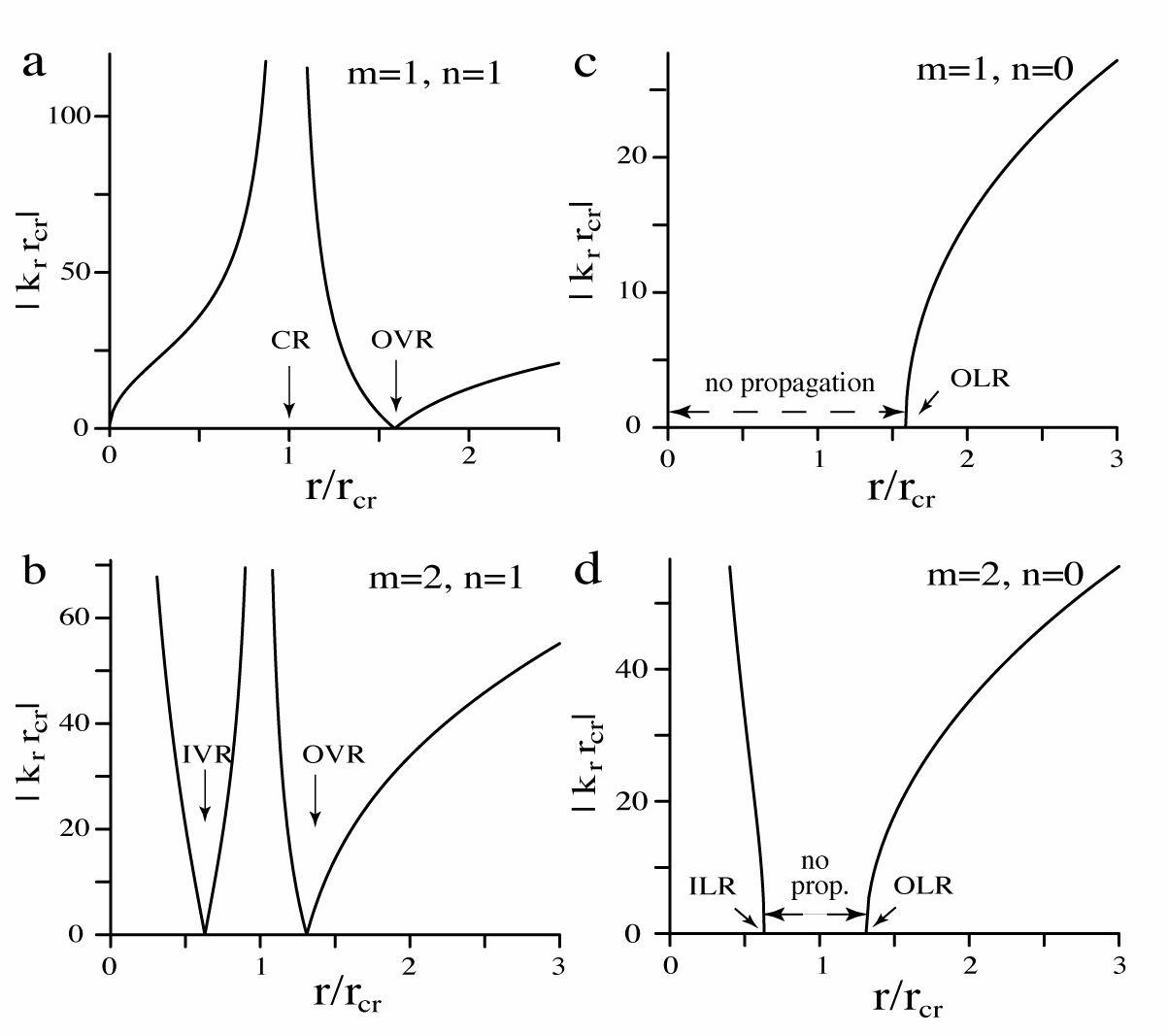
Figure 23: Radial wavenumber $k_{r}$ as a function of radius $r$ for a thin Keplerian disc with $h/r=c_{s}/(r\Omega)=0.05$, where $r_{cr}$ is the corotation radius. Panels (a) and (b) are for the bending waves, while (c) and (d) are for the density waves.

A.1 m=1 Bending Wave

For a one-armed ($m=1$) bending wave ($n=1$) of a Keplerian disc ($\kappa=\Omega$ and $\Omega_{\perp}=\Omega$) equation (4) can be written as

$$\left\{\left({k_{r}c_{s}\over\Omega}\right)^{2}-\left[\left({\tilde{\omega}\over\Omega}\right)^{2}-1\right]\left[1-\left({\Omega\over\tilde{\omega}}\right)^{2}\right]\right\}z_{w}=0,$$ (15)

where $\tilde{\omega}=\omega-\Omega$ and the other parameters are defined in Sec. 2.

We find that the WKBJ equation (3) is a good approximation to the full wave solution except for the region where $|k_{r}r_{cr}|$ is small or the wavelength is long. Specifically, the approximation is reasonable for $|k_{r}r_{cr}|\gtrsim 4.94$. For $|k_{r}r_{cr}|<5$, equation (A1) is solved as a differential equation for $z_{w}$ obtained by setting $k_{r}^{2}\rightarrow-d^{2}/dr^{2}$.

Panel (a) of Figure A1 shows the radial dependence of $|k_{r}r_{cr}|$ for a disc with constant fractional half-thickness $h/r=c_{s}/(r\Omega)=0.05$ and $\omega=\Omega(r_{cr})$. The corotation resonance where $\tilde{\omega}=0$ and $k_{r}^{2}\rightarrow\infty$ is at $r=r_{cr}$. The vertical/Lindblad resonance where $\tilde{\omega}=\Omega$ and $k_{r}^{2}=0$ is at $r=2^{2/3}r_{cr}\approx 1.59r_{cr}$. For $r/r_{cr}\rightarrow 0,$ $k_{r}r_{cr}\rightarrow 2(r/h)\sqrt{r/r_{cr}}$. For $r/r_{cr}\rightarrow 1,$ $k_{r}r_{cr}\rightarrow(r/h)|(r/r_{cr})^{3/2}-1|^{-1}$. For $r/r_{cr}\rightarrow\infty,$ $k_{r}r_{cr}\rightarrow(r/h)\sqrt{r/r_{cr}}$.

We refer to the warp in the range $r/r_{cr}<1$ as the ‘inner warp.’ For most of the range $r/r_{cr}<1$ (excluding very small $r/r_{cr}$), the amplitude of the inner warp is well approximated by equation (A2). Fig. A2 (left panel) shows the real and imaginary parts of the warp profile at $\phi=0$. Next panel to the right shows the top view of $\Re[z_{w}(r,\phi)]$ of the inner warp. The warp becomes very tightly wrapped as $r/r_{cr}$ increases towards unity. Approximately, $\phi\sim-(2r/3h)\ln[r_{cr}/(r_{cr}-r)]$ and $|z_{w}|\sim\sqrt{r_{cr}-r}$ as $r\rightarrow r_{cr}$.

In the range $r/r_{cr}>0$ we refer to warp as the ‘outer warp’. Fig. A2 (3rd panel) shows the real and imaginary parts of $z_{w}$ at $\phi=0$. As $r\rightarrow r_{cr}$.$|z_{w}|\sim\sqrt{r-r_{cr}}$ while for $r\gg r_{cr}$ $|z_{w}|\sim r^{-1/4}$. Fig. A2 (right panel) shows the top view of $\Re[z_{w}(r,\phi)]$.

A.2 m=2 Bending Wave

Using the WKBJ approximation to equation (2) for a two-armed ($m=2$) warp ($n=1$) of a Keplerian disc gives

$$|k_{r}r_{cr}|={r\over h}{1\over\bar{r}}\bigg{[}[(\bar{r}^{3/2}-1)^{2}-{1/4}][4-(\bar{r}^{3/2}-1)^{-2}]\bigg{]}~{},$$ (16)

where $\bar{r}\equiv r/r_{cr}$ with $r_{cr}$ the corotation radius, so that $\omega=m\Omega(r_{cr})$. Note that $k_{r}=0$ at the inner and outer vertical resonances (IVR and OVR) at $\bar{r}=(1\pm 1/2)^{2/3}\approx 0.630,~{}1.31$, and that $|k_{r}|\rightarrow\infty$ at the corotation resonance at $\bar{r}=1$. Panel (b) of Fig. A1 shows the radial dependence of $k_{r}$ for a sample case.

A.3 In-plane modes, $n=0$ (Density Waves)

The WKBJ solution of equation (2) for $n=0$, $m=1,~{}2$, and a Keplerian disc gives

$$\tilde{\omega}^{2}=\Omega^{2}+k_{r}^{2}c_{s}^{2}~{},$$ (17)

where we have set $\kappa=\Omega$. For a disc with $c_{s}/(r\Omega)=h/r=$ const, one finds

$$|k_{r}r_{cr}|=(r/h)(1/\bar{r})\left[m^{2}(\bar{r}^{3/2}-1)^{2}-1\right]^{1/2}~{},$$ (18)

where $\bar{r}\equiv r/r_{cr}$ with $r_{cr}$ being the corotation radius, $\omega=m\Omega(r_{cr})$. For the one-armed mode ($m=1$), there are real values of $k_{r}$ only for $r/r_{cr}\geq 2^{2/3}\approx 1.59$, which is the outer Lindblad resonance.

For the two-armed mode ($m=2$), there are real values of $k_{r}$ only for $r/r_{cr}\leq 2^{-2/3}\approx 0.63$ (the inner Lindblad resonance) and for $r/r_{cr}\geq 1.5^{2/3}\approx 1.311$ (the outer Lindblad resonance). Panels (c) and (d) show the the radial dependencies of $k_{r}$ for the two cases.

Appendix B Radially trapped modes

A radially localized, in-plane instability of discs for $m=1,~{}2,..$ know as the ‘Rossby wave instability’ (RWI) may occur near regions where there is an extremum (as a function of $r$) of the entropy and/or the potential vorticity $\hat{\bf z}\cdot(\nabla\times{\bf v})/\Sigma$, where ${\bf v}$ is the disc velocity and $\Sigma$ is the disc’s surface mass density (Lovelace et al., 1999; Li et al., 2000; Lovelace et al., 2009; Lovelace & Romanova, 2007); see also Lovelace & Hohlfeld (1978). Radially trapped modes in discs around black holes were analyzed earlier by Nowak & Wagoner (1991). Of particular interest here is the RWI in the non-Keplerian region of a disc (Lovelace et al. 2009; hereafter LTR09) which occurs when a disc encounter the magnetosphere of a slowly-rotating star. An example of such a rotation curve is shown in Figure B1. For given profiles of $v_{\phi}$, $\rho$, etc. and a given $m$, the value of the growth rate is found by solving for the ‘ground state’ solution of Schrödinger-like equation for the enthalpy perturbation $\psi$,

$${d^{2}\psi\over dr^{2}}=U(r|\omega)\psi~{},$$ (19)

where $U(r|\omega)$ is an effective potential (LTR09) shown for a sample case in Figure B2. The ground state is found by varying both the real and imaginary parts of the mode frequency $\omega$ so as to give the $\psi(r)$ most deeply trapped in the potential well. For typical profiles and $m=1$, the growth rate is $\omega_{i}\sim 0.1(v_{\phi}/r)_{R}$ and the real part of the frequency is $\omega_{r}\approx(v_{\phi}/r)_{R}$, where the $R-$subscript indicates evaluation at the resonant radius $r_{R}$. The radial width of the mode is $\Delta r/r_{R}\sim 0.05$.

The linear growth of the Rossby wave is predicted to saturate when the azimuthal frequency of trapping of a fluid particle in the trough of the wave $\omega_{T}$ grows to a value equal to the growth rate $\omega_{i}$ as discussed by LTR09. For the $m=1$ mode the saturation level is estimated as $|\delta\rho|/\rho\sim 1.4(\omega_{i}/\omega_{r})^{2}(r/h)$ (LTR09).

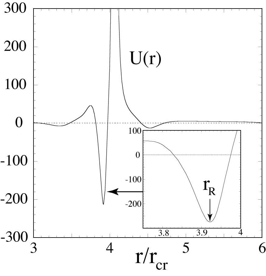
Figure 25: Left panel: Midplane radial dependencies of the azimuthal disc velocity $v_{\phi}$, magnetic field $B_{z}$, and density $\rho$, where $v_{K}$ is the Keplerian velocity. The vertical arrow indicating $r_{R}$ is the location of the bottom of a potential well $U(r)$ shown in right panel (from LTR09). Right panel: Effective potential $U(r)$ for the profiles shown in Figure D1 from LTR09.

References

- Alencar et al. (2010) Alencar, S. H. P., Teixeira, P. S., Guimar es, M. M., McGinnis, P. T., Gameiro, J. F., Bouvier, J., Aigrain, S., Flaccomio, E., Favata, F. 2010, A&A, 519, A88
- Alpar & Psaltis (2005) Alpar, M.A. & Psaltis, D. 2005, arXiv:astro-ph/0511412
- Alpar & Psaltis (2008) Alpar, M.A. & Psaltis, D. 2008, MNRAS, 391, 1472
- Aly (1980) Aly, J.J. 1980, A&A, 86, 192
- Armitage (2002) Armitage, P. 2002, ApJ, 330, 895
- Arons & Lea (1976) Arons, J. & Lea, S.M. 1976, ApJ, 207, 914
- Balbus & Hawley (1991) Balbus, S.A. & Hawley, J. F. 1991, ApJ, 376, 214
- Bachetti et al. (2010) Bachetti, M., Romanova, M. M., Kulkarni, A. K., Burderi, L., di Salvo, T., 2010, MNRAS, 403, 1193
- Barret et al. (2006) Barret, D., Olive, J.-F., & Miller, M.C. 2006, MNRAS, 370, 1140
- Belloni et al. (2002) Belloni, T., Psaltis, D., & van der Klis, M. 2002, ApJ, 572, 392
- Belloni et al. (2007) Belloni, T., Méndez, M., & Homan, J. 2007, MNRAS, 376, 1133
- Boutloukos et al. (2006) Boutloukos, S., van der Klis, M., Altamirano, D., Klein-Wolt, M., Wijnands, R., Jonker, P. G., Fender, R. P. 2006, ApJ, 653, 1435
- Bouvier et al. (1999) Bouvier, J., Chelli, A., Allain, S., Carrasco, L., Costero, R., Cruz-Gonzalez, I., Dougados, C., Fern ndez, M. et al. 1999, A&A, 349, 619
- Bouvier et al. (2003) Bouvier, J., Grankin, K. N., Alencar, S. H. P., Dougados, C., Fern ndez, M., Basri, G., Batalha, C., Guenther, E. et al. 2003, A&A, 409, 169
- Bouvier et al. (2007a) Bouvier, J., Alencar, S. H. P., Harries, T. J., Johns-Krull, C. M. & Romanova, M. M. 2007a, Protostars and Planets V, B. Reipurth, D. Jewitt, and K. Keil (eds.), University of Arizona Press, Tucson, 479
- Bouvier et al. (2007b) Bouvier, J., Alencar, S. H. P., Boutelier, T., Dougados, C., Balog, Z., Grankin, K., Hodgkin, S. T., Ibrahimov, M. A. 2007b, A&A, 463, 1017
- Carpenter et al. (2001) Carpenter, J.M., Hillenbrand, L.A., & Skrutskie, M.F. 2001, AJ, 121, 3160
- Donati et al. (2010) Donati, J.-F., Skelly, M. B., Bouvier, J., Gregory, S. G., Grankin, K. N., Jardine, M. M., Hussain, G. A. J., Ménard, F. et al. 2010, MNRAS, 409, 1347
- Donati (2011) Donati, J.-F., Bouvier, J., Walter, F. M., Gregory, S. G., Skelly, M. B., Hussain, G. A. J., Flaccomio, E., Argiroffi, C. et al. 2011, MNRAS, 412, 2454
- Fragile & Anninos (2005) Fragile, P.C., & Anninos, P., 2005, ApJ, 623, 347
- Fragile et al. (2007) Fragile, P.C., Blaes, O.M., Anninos, P., & Salmonson, J.D. 2007, ApJ, 668, 417
- Fu & Lai (2012) Fu, W., & Lai, D. 2012, MNRAS, 423, 831
- Goldreich (1978) Goldreich, P., & Tremaine, S. 1978, ApJ, 222, 850
- Herbst et al. (2002) Herbst, W., Bailer-Jones, C.A.L. and Mundt, R. et al. 2002, AAP, 396, 513
- Hawley (2000) Hawley, J.F. 2000, ApJ, 528, 462
- Kaisig et al. (1992) Kaisig, M., Tajima, T., & Lovelace, R.V.E. 1992, ApJ, 386, 83
- Kato et al. (1998) Kato, S., Fukue, J., & Mineshige, S. 1998, “Black-Hole Accretion Disks” (Kyoto University Press: Kyoto Japan)
- Kato (2004) Kato, S. 2004, PASJ, 56, 905
- Kato (2008) Kato, S. 2008, PASJ, 60, 111
- Kato (2010) Kato, S. 2010, PASJ, 61, 1237
- Kluzniak & Abramowicz (2002) Kluzniak, W. & Abramowicz, M.A. 2002, arXiv:astro-ph/0203314v2
- Koldoba et al. (2002) Koldoba, A. V., Romanova, M. M., Ustyugova, G. V., Lovelace, R. V. E. 2002, ApJ, 576, L53
- Koldoba et al. (2008) Koldoba, A. V., Romanova, M. M., Ustyugova, G. V., Lovelace, R. V. E. 2008, MNRAS, 388, 357
- Kulkarni & Romanova (2008) Kulkarni, A., & Romanova, M.M. 2008, ApJ, 386, 673
- Kulkarni & Romanova (2009) Kulkarni, A., & Romanova, M.M. 2009, ApJ, 398, 1105
- Lai (1999) Lai, D. 1999, ApJ, 524, 1030
- Lai & Zhang (2008) Lai, D. & Zhang, H. 2008, ApJ, 683, 949
- Lamb et al. (1985) Lamb, F.K., Shibazaki, N., Alpar, M. A., & Shaham, J. 1986, Nature, 317, 681
- Lamb & Miller (2003) Lamb, F.K. & Miller, M.C. 2003, arXiv: astro-ph/0308179v1
- Li et al. (2000) Li, H., Finn, J.M., Lovelace, R.V.E., & Colgate, S.A. 2000, ApJ, 533, 1023
- Lipunov (1980) Lipunov, V.M. 1980, SvAL, 6, 14
- Long et al. (2005) Long, M., Romanova, M.M., & Lovelace, R.V.E. 2005, ApJ, 634, 1214
- Lovelace & Hohlfeld (1978) Lovelace, R.V.E., & Hohlfeld, R.G. 1978, ApJ, 221, 51
- Lovelace et al. (1999) Lovelace, R.V.E., Li, H., Colgate, S.A., & Nelson, A.F. 1999, ApJ, 513, 805
- Lovelace & Romanova (2007) Lovelace, R. V. E. & Romanova, M. M. 2007, ApJ, 670, L13
- Lovelace et al. (2009) Lovelace, R. V. E., Turner, L. & Romanova, M. M. 2009, ApJ, 701, 225
- Lubow (1981) Lubow, S.H. 1981, ApJ, 245, 274
- Méndez et al. (1998) Méndez, M., & van der Klis, M., & van Paradijs, J. 1998, ApJ, 506, L117
- Méndez & Belloni (2007) Méndez, M., & Belloni 2007, MNRAS, 381, 790
- Miller, Lamb & Psaltis (1998) Miller, M.C., Lamb, F.K., & Psaltis, D. 1998, ApJ, 508, 791
- Nelson & Papaloizou (2000) Nelson, R.P., & Papaloizou, J.C.B. 2000, MNRAS, 315, 570
- Nowak & Wagoner (1991) Nowak, M.A., & Wagoner, R.V. 1991, ApJ, 378, 656
- Ogilvie (1999) Ogilvie, G.I. 1999, MNRAS, 304, 557
- Ogilvie (2006) Ogilvie, G.I. 2006, MNRAS, 365, 977
- Okazaki et al. (1987) Okazaki, A. T., Kato, S., & Fukue, J. 1987, PASJ, 39, 457
- O’Neil et al. (2009) O’Neill, S.M., Reynolds, C.S., Miller, M.C. 2009, ApJ, 693, 1100
- Papaloizou & Lin (1995) Papaloizou J. C. B., & Lin D. N. C. 1995, ApJ, 438, 841
- Petri (2005) Petri, J. 2005, A&A, 439, 443
- Pfeiffer & Lai (2004) Pfeiffer, H.P., & Lai. D. 2004, ApJ, 204,766
- Patterson (1981) Patterson, J. 1981, ApJ Suppl, 45, 517
- Powell (1999) Powell, K.G., Roe, P.L., Linde, T.J., Gombosi, T.I., & De Zeeuw, D.L. 1999, J. Comp. Phys., 154, 284
- Pretorius et al. (2006) Pretorius, M.L., Warner, B., & Woudt, P.A. 2006, MNRAS, 368, 361
- Robinson & Nather (1979) Robinson, E.L., & Nather, R.E. 1979, ApJ Suppl, 39, 461
- Romanova et al. (2002) Romanova, M.M., Ustyugova, G.V., Koldoba, A.V., & Lovelace, R.V.E. 2002, ApJ, 578, 420
- Romanova et al. (2003) Romanova, M.M., Ustyugova, G.V., Koldoba, A.V., & Lovelace, R.V.E. 2003, ApJ, 595, 1009
- Romanova et al. (2004) Romanova, M.M., Ustyugova, G.V., Koldoba, A.V., & Lovelace, R.V.E. 2004, ApJ, 610, 920
- Romanova & Kulkarni (2009) Romanova, M.M. & Kulkarni, A.K. 2009, MNRAS, 398, 701
- Romanova et al. (2008) Romanova, M.M., Kulkarni, A.K., Lovelace, R.V.E. 2008, ApJ Letters, 273, L171
- Romanova et al. (2012) Romanova, M.M., Ustyugova, G.V., Koldoba, A.V., & Lovelace, R.V.E. 2012, ApJ, 421, 63
- Reynolds & Miller (2009) Reynolds, C.S., & Miller, M.C. 2009, ApJ, 692, 869
- Rucinski et al. (2008) Rucinski, S.M., Matthews, J.M., Kuschnig, R., Pojmanski, G., Rowe, J., Guenther, D. B., Moffat, A,F.,J., Sasselov et al. 2008, MNRAS, 391, 1913
- Shakura & Sunyaev (1973) Shakura, N.I., & Sunyaev, R.A. 1973, A&A, 24, 337
- Spruit et al. (1995) Spruit, H. C., Stehle, R., & Papaloizou, J. C. B., 1995, MNRAS, 275, 1223
- Spruit & Taam (1990) Spruit, H. C. & Taam, R. E. 1990, A&A, 229, 475
- Stella & Vietri (1999) Stella, L., & Vietri, M. 1999, Phys. Rev. Lett., 82, 17
- Tanaka (1994) Tanaka, T. 1994, J. Comp. Phys., 111, 381
- Tanaka et al. (2002) Tanaka, H., Takeuchi, T., & Ward, W.R. 2002, ApJ, 565, 1257