Nonequilibrium probe of paired electron pockets in the underdoped cuprates

Abstract

We propose an experimental method that can be used generally to test whether the cuprate pseudogap involves precursor pairing that acts to gap out the Fermi surface. The proposal involves angular-resolved photoemission spectroscopy (ARPES) performed in the presence of a transport current driven through the sample. We illustrate this proposal with a specific model of the pseudogap that contains a phase-incoherent paired electron and unpaired hole Fermi surfaces. We show that even a weak current tilts the paired band and reveals parts of the previously gapped electron Fermi surface in ARPES if the binding energy is smaller but close to the pseudogap. Stronger currents can also reveal the Fermi surface through direct suppression of pairing. The proposed experiment is sufficiently general such that it can be used to reveal putative Fermi surfaces that have been reconstructed from other types of periodic order and are gapped out due to pairing. The observation of the predicted phenomena should help resolve the central question about the existence of pairs in the enigmatic pseudogap regime.

I Introduction

The experimental and theoretical effort to understand the pseudogap phase of the underdoped cuprate superconductors has lasted for decades Timusk and Statt (1999); Norman and Pepin (2003); Norman et al. (2005); Lee et al. (2006); Sebastian et al. (2012). Most of the current proposed explanations for the phase can be classified into one of two seemingly separate scenarios. One scenario interprets the pseudogap as a superconducting precursor state in which electrons pair incoherently above $T_{c}$ eme ; Banerjee et al. (2011), and is supported by some transport Cor , Nernst Wang et al. (2006), and proximity effect Yuli et al. (2009) experiments. The other links the pseudogap to an ordering phenomenon that competes with superconductivity. Evidence for this scenario includes angle-resolved photoemission (ARPES) Marshall et al. (1996); ARP ; Has ; Damascelli et al. (2003), electrical transport Lib , quantum oscillations Doiron-Leyraud et al. (2007); Sebastian et al. (2008); Yelland et al. (2008); Bangura et al. (2008), x-ray diffraction Liu et al. (2008); Wilkins et al. (2011), neutron scattering studies Stock et al. (2005); Haug et al. (2009); Wilkins et al. (2011), and STM Hoffman et al. (2002); han ; Kohsaka et al. (2007); CDW ; koh . Recently, observations that support charge density wave (CDW) ordering have been reported in NMR hig and x-ray scattering Ghiringhelli et al. (2012); Chang et al. (2012); LeBoeuf et al. (2012) experiments. Although the two scenarios are typically treated as separate interpretations of the pseudogap, the phenomena of paired excitations and competing order are not necessarily mutually exclusive. In La-based cuprates, for instance, there is evidence for the simultaneous presence of a competing order lak ; Tranquada et al. (2004); Khaykovich et al. (2005); Chang et al. (2008, 2009) and pairing Wang et al. (2006); Yuli et al. (2009). The coexistence of the two phenomena has also served as a basis for some theoretical models of the pseudogap chu ; Galitski and Sachdev (2009).

Whether precursor pairing exists in conjunction with competing order in the pseudogap regime is an important question. Here, we propose and model an experiment that can help resolve this question by directly testing whether the pseudogap contains any putative (or “ghost”) Fermi surfaces that are gapped out specifically due to pairing. The recent quantum oscillation and photoemission experiments on the cuprates give an impetus to investigate a pseudogap scenario in which both pairing and competing order are incorporated simultaneously. While quantum oscillations in the pseudogap regime provide evidence for coherent electron Fermi pockets at finite magnetic fields LeBoeuf et al. (2007), evidence for such pockets is not observed in photoemission at zero magnetic field Shen et al. (2005); hos ; Tranquada et al. (2010). However, these observations can be reconciled with a scenario in which parts of the putative Fermi surfaces evade photoemission detection due to a strong pairing gap, which in turn is suppressed by a finite magnetic field. This restores the previously hidden Fermi surfaces and gives rise to the observed quantum oscillations. A rigorous microscopic theory for such a scenario was recently developed in Ref. Galitski and Sachdev, 2009, but a direct experimental test of the scenario is still lacking.

In this work, we propose an ARPES experiment performed while a transport current is driven through the sample. We show that an arbitrarily weak current can shift the quasiparticle spectrum and reveal the hidden paired bands which should appear as new Fermi surfaces in ARPES. The specific way in which the current shifts the spectrum would also be indicative of a gap originating from pairing. For these weak currents, the heating and the influence of the current-induced magnetic field on the path of the photo-ejected electron should be small. Large currents can lead to complete depairing, and this should, in principle, also reveal the hidden Fermi surfaces. However, such large currents may be impractical due to Joule heating and magnetic field effects. To illustrate our proposal, we apply the method to a particular theoretical model Galitski and Sachdev (2009), in which the pseudogap emerges from a fluctuating critical antiferromagnetic state with paired electron and unpaired hole pockets in the anti-nodal and nodal regions, respectively. We emphasize that the applicability of the proposed method is not limited to the model, but can be generally used to test the existence of putative Fermi surfaces that have been reconstructed due to other types of order Sebastian et al. (2012), including CDW Ghiringhelli et al. (2012); Chang et al. (2012); LeBoeuf et al. (2012), but are gapped out due to pairing. The main idea of our proposal may also be useful when considering the application of transport current in conjunction with other spectroscopic techniques that probe electronic structure.

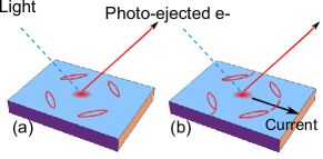
Figure 1: (color online) A qualitative illustration of the experimental setup and the predicted phenomenon: (a) the incident light and ejected electrons that initially leave the electron pockets hidden due to a pairing gap; (b) the electron-pockets are partially revealed in the ARPES signal due to a current running through the sample along the anti-nodal direction.

II Model

To be concrete, we illustrate our proposal using a model of the pseudogap presented in Ref. Galitski and Sachdev, 2009. The model is supported by three recent experimental developments. First, recent work has observed a proximity-induced pseudogap Yuli et al. (2009) and supports the idea that the pseudogap is connected to paired quasiparticles. Second, the experimental discovery Doiron-Leyraud et al. (2007); LeBoeuf et al. (2007); Sebastian et al. (2008) of small Fermi pockets in the pseudogap phase of underdoped cuprates motivates a description which incorporates Fermi surface reconstruction. Third, there is a nodal-anti-nodal dichotomy Yoshida et al. (2003); Zhou et al. (2004); Shen et al. (2005); Tanaka et al. (2006) observed in STM Pushp et al. (2009) and Raman  Le Tacon et al. (2006) experiments, where nodal excitations have an energy which decreases with decreasing doping, and anti-nodal excitations have a larger energy that increases with decreasing doping. These key ingredients, namely pairing, Fermi surface reconstruction, and the nodal-anti-nodal dichotomy, are incorporated in the theory proposed in Ref. Galitski and Sachdev, 2009.

According to the theory, the pseudogap phase emerges from a strongly fluctuating critical antiferromagnetic state with reconstructed Fermi-surfaces consisting of electron-like pockets in the anti-nodal regions $(\pi/a,0)$ and $(0,\pi/a)$ and hole-like pockets in the nodal regions $(\pm\pi/2a,\pm\pi/2a)$. The components of the physical electron are described in a rotated reference frame set by the local spin-density wave (SDW) order ${\boldsymbol{\varphi}}=z^{*}_{\sigma}{\boldsymbol{\sigma}}_{\sigma\sigma^{\prime}}z_{\sigma^{\prime}}$, where the bosonic spinon field $z_{\sigma}$ defines the SU(2) rotation. This parametrization gives rise to an emergent gauge field, which plays a crucial role in the pairing of the fermions. The pseudogap phase is characterized by strongly $s$-wave paired (but uncondensed) electron pockets and hole pockets foo that remain unpaired (a weak $p$-wave pairing in the hole pockets is assumed to be suppressed by temperature). This is shown to be equivalent to $d$-wave pairing when the Brillouin zone is unfolded Geshkenbein et al. (1997); Galitski and Sachdev (2009); Sensarma and Galitski (2011). Also, the apparent discrepancy between full pockets in the nodal regions and the Fermi arcs observed in ARPES can be reconciled with a model Kaul et al. (2007) that is consistent with what we consider here Galitski and Sachdev (2009). To reiterate, it is possible that the quantum oscillation experiments Doiron-Leyraud et al. (2007); Sebastian et al. (2008) are observing anti-nodal electron pockets, which are paired at zero field, but are driven normal by the magnetic field. We show that our proposal can falsifiably test this paired electron pocket scenario on Ref. Galitski and Sachdev, 2009 at zero field.

III Theory

We consider a hole-doped cuprate superconductor in the pseudogap regime subjected to a uniform current ${\boldsymbol{J}}$ as shown in Fig. 1(b). Our main goal is to determine key qualitative features of an ARPES spectrum measured in the presence of the current. A minimal model, which is consistent with the model in Ref. Galitski and Sachdev, 2009 and captures the key features necessary to address an ARPES experiment in the presence of current, is

$$H=\sum_{{\boldsymbol{k}}\in RBZ}\sum_{\alpha=\pm}\left[\xi_{{\boldsymbol{k}}f}f^{\dagger}_{{\boldsymbol{k}}\alpha}f_{{\boldsymbol{k}}\alpha}+\xi_{{\boldsymbol{k}}h}h^{\dagger}_{{\boldsymbol{k}}\alpha}h_{{\boldsymbol{k}}\alpha}\right]\\ -\sum_{{\boldsymbol{k}}\in RBZ}\left[\Delta f^{\dagger}_{{\boldsymbol{k}}+}f^{\dagger}_{-{\boldsymbol{k}}-}+h.c.\right]+\frac{\Delta^{2}}{\lambda},$$ (1)

where $f_{{\boldsymbol{k}}\pm}$ and $h_{{\boldsymbol{k}}\pm}$ are the annihilation operators for the electron-like and hole-like excitations with momentum ${\boldsymbol{k}}$, respectively, and $\pm$ labels the charge associated with the emergent gauge field. We note that $f_{{\boldsymbol{k}}\alpha}$ becomes the physical electron in the SDW ordered state, where the spinon field $z_{\sigma}$ condenses and the $\pm$ indices become equivalent to the electron spin indices. Pairing in the electron pockets is included at the mean-field level by introducing a real $s$-wave pair potential $\Delta$. The spectra are given by $\xi_{{\boldsymbol{k}}f,h}=(\xi_{{\boldsymbol{k}}}+\xi_{{\boldsymbol{k}}+{\boldsymbol{Q}}})/2\pm[(\xi_{{\boldsymbol{k}}}-\xi_{{\boldsymbol{k}}+{\boldsymbol{Q}}})^{2}+4\varphi^{2}]^{1/2}/2$, where $\xi_{\boldsymbol{k}}=-2t(\cos k_{x}a+\cos k_{y}a)-4t^{\prime}\cos k_{x}a\cos k_{y}a-\mu$. Here, ${\boldsymbol{Q}}=(\pi/a,\pi/a)$, and we will take $t^{\prime}=-0.3t$ and $\mu=-0.6t$ Hashimoto et al. (2008). The quantity $\varphi$ is the uniform SDW order parameter, but we stress that $\varphi$ is used here merely to parameterize the underlying Brillouin zone folding, and that in reality, spin fluctuations are expected to suppress long-range antiferromagnetic order in the pseudogap phase. In the above, $\lambda>0$ is the effective attractive interaction for the electrons generated by the gauge fluctuations. Since the pseudogap phase is not characterized by long-range SDW order the attractive interaction mediated by the gauge fluctuations is, in principle, long-ranged Galitski and Sachdev (2009).

We emphasize here that a calculation of the current within model (1) would give rise to a phase-coherent superflow, which is not correct in the pseudogap regime. However, the excitation spectrum in the presence of current should be correctly obtained from these expressions and can reliably calculate the spectral function, which is the central quantity of interest.

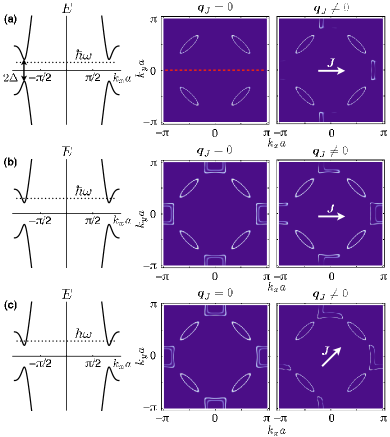
Figure 2: (color online) Spectral function at zero and finite current for binding energy $\hbar\omega$ (a) just below and (b) above $E_{\boldsymbol{k}}$. As indicated by the white arrows, the current is applied along the anti-nodal direction in (a) and (b), and the nodal direction in (c). Paired bands on the left are plotted along the red dashed line. An arbitrarily small $q_{J}$ can reveal or erase parts of the electron pockets as long as the binding energy is tuned close to the edge of a paired band.

IV Results

IV.1 Spectral function for a current-carrying pseudogap

Transport in the pseudogap can be thought of as a dissipative flow of holons and charge $2e$ bosons. A weak current will only lead to a simple shift in the holon Fermi surface by an amount $eE\tau_{h}/\hbar$, where $\tau_{h}$ is the hole transport relaxation time. This does not lead to a dramatic change in the hole spectral function. As we show below, the presence of even a weak current leads to a noticeable modification in the spectral function for the electron sector, namely, the current can cause sections of the hidden paired electron band to appear or disappear.

The current endows the Cooper pairs with a center-of-mass momentum ${\boldsymbol{q}}_{\boldsymbol{J}}$, and the single-particle Green function in the presence of a uniform current can be written as mak ; Maki and Tsuneto (1962)

$$\check{G}_{\boldsymbol{k}}(i\omega_{n})=\left[\hbar(i\omega_{n}-{\boldsymbol{v}_{\boldsymbol{k}}}\cdot{\boldsymbol{q}}_{\boldsymbol{J}})\check{1}-\xi_{{\boldsymbol{k}}f}\check{\tau}_{3}+\Delta\check{\tau}_{1}\right]^{-1},$$ (2)

where $\omega_{n}=(2n+1)\pi k_{B}T$ are the fermionic Matsubara frequencies, ${\boldsymbol{v}_{\boldsymbol{k}}}=\partial\xi_{{\boldsymbol{k}}f}/\hbar\partial{\boldsymbol{k}}$, checks indicate matrices in Nambu space, and $\check{\tau}_{i}$ are the Pauli matrices. The gap is then obtained from the following self-consistent condition,

$$1=\frac{\lambda}{N}\sum_{{\boldsymbol{k}}}\frac{1-n_{F}(E^{+}_{{\boldsymbol{k}}})-n_{F}(E_{{\boldsymbol{k}}}^{-})}{2E_{{\boldsymbol{k}}}},$$ (3)

where $n_{F}$ is the Fermi-Dirac distribution function and $E^{\pm}_{{\boldsymbol{k}}}=E_{\boldsymbol{k}}\pm\hbar{\boldsymbol{v}_{\boldsymbol{k}}}\cdot{\boldsymbol{q}}_{\boldsymbol{J}}=[\xi_{{\boldsymbol{k}}f}^{2}+\Delta^{2}]^{1/2}\pm\hbar{\boldsymbol{v}_{\boldsymbol{k}}}\cdot{\boldsymbol{q}}_{\boldsymbol{J}}$. The retarded Green function for the $f_{{\boldsymbol{k}}+}$ electrons, $G^{R}_{{\boldsymbol{k}}+}(\omega)$, then defines the corresponding spectral function $A_{{\boldsymbol{k}}+}(\omega)=-\mbox{Im}G^{R}_{{\boldsymbol{k}}+}(\omega)/\pi$. One then finds,

$$A_{{\boldsymbol{k}}+}(\omega)=s^{2}_{\boldsymbol{k}}\delta(\hbar\omega-\xi_{{\boldsymbol{k}}h})\\ +r^{2}_{\boldsymbol{k}}\left[u^{2}_{\boldsymbol{k}}\delta(\hbar\omega-E^{+}_{\boldsymbol{k}})+v^{2}_{\boldsymbol{k}}\delta(\hbar\omega+E^{-}_{\boldsymbol{k}})\right],$$ (4)

where $r^{2}_{\boldsymbol{k}}=[1+(\xi_{\boldsymbol{k}}-\xi_{{\boldsymbol{k}}+{\boldsymbol{Q}}})/(\xi_{{\boldsymbol{k}}f}-\xi_{{\boldsymbol{k}}h})]/2$ and $s^{2}_{\boldsymbol{k}}=[1-(\xi_{\boldsymbol{k}}-\xi_{{\boldsymbol{k}}+{\boldsymbol{Q}}})/(\xi_{{\boldsymbol{k}}f}-\xi_{{\boldsymbol{k}}h})]/2$, and the Bogoliubov coherence factors are given by $u^{2}_{\boldsymbol{k}}=(1+\xi_{{\boldsymbol{k}}f}^{2}/E_{\boldsymbol{k}})/2$ and $v^{2}_{\boldsymbol{k}}=(1-\xi_{{\boldsymbol{k}}f}^{2}/E_{\boldsymbol{k}})/2$. Although there can be considerable broadening of the spectral peaks in the pseudogap regime, our proposal should not be heavily limited by a lack of resolution because one needs to identify merely the presence or absence of the putative Fermi surfaces. Therefore, (4) should correctly convey the main qualitative effects of the applied current on the spectral function.

IV.2 Spectral function for weak currents

From (4) we see that the spectral function is non-zero when either (i) $\hbar\omega-\hbar{\boldsymbol{v}_{\boldsymbol{k}}}\cdot{\boldsymbol{q}}_{\boldsymbol{J}}-E_{{\boldsymbol{k}}}=0$ or (ii) $\hbar\omega-\hbar{\boldsymbol{v}_{\boldsymbol{k}}}\cdot{\boldsymbol{q}}_{\boldsymbol{J}}+E_{{\boldsymbol{k}}}=0$. The effect of the Doppler shift is to move the energy scale $\hbar\omega$ away or towards the quasiparticle bands $\pm E_{\boldsymbol{k}}$ depending on the sign of $\hbar{\boldsymbol{v}_{\boldsymbol{k}}}\cdot{\boldsymbol{q}}_{\boldsymbol{J}}$. All that is required here is to use a small $\hbar{\boldsymbol{v}_{\boldsymbol{k}}}\cdot{\boldsymbol{q}}_{\boldsymbol{J}}$ to just cross into either of the $\pm E_{{\boldsymbol{k}}}$ bands as long as the binding energy is tuned near the edge of a band. In Fig. 2, we plot the spectral function (4) at binding energies just below [Fig. 2(a)] and above [Fig. 2(b)] the upper paired band for zero and finite current. We consider the case where the current is applied in the anti-nodal direction, and also in the nodal direction [Fig. 2(c)]. Plotted on the left are a cut of the paired band dispersion along the $k_{y}=0$ line in the Brillouin zone (indicated by the red dashed line on the right in (a)), and the binding energies are indicated by the dotted lines. In (a), the binding energy is set inside the gap at zero current and hence the electron pockets are initially not observed. However, once the current is applied, the paired spectrum at ${\boldsymbol{k}}$ points where ${\boldsymbol{v}_{\boldsymbol{k}}}$ is parallel to ${\boldsymbol{q}}_{\boldsymbol{J}}$ is shifted up in energy while the spectrum at ${\boldsymbol{k}}$ points where ${\boldsymbol{v}_{\boldsymbol{k}}}$ is anti-parallel to ${\boldsymbol{q}}_{\boldsymbol{J}}$ is shifted down in energy. This leads to the appearance of some sections of the electron pockets. In Figs. 2(b),(c) the binding energy crosses both the hole and the upper paired bands. The application of the current here leads to the disappearance of some sections of the electron pockets.

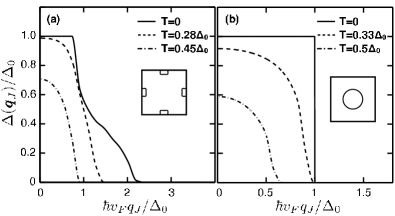
Figure 3: Solution to the gap equation (3) as a function of $q_{J}$ along the anti-nodal direction. In (a), the solution is obtained for electrons with spectrum $\xi_{{\boldsymbol{k}}f}$ (with the putative Fermi surface shown in the inset), while in (b) we consider the regular isotropic spectrum $\xi^{0}_{\boldsymbol{k}}=\hbar^{2}k^{2}/2m-\mu$ (with the circular putative Fermi surface). The gap is normalized with respect to its value at zero temperature and zero current.

IV.3 Depairing due to strong currents

A strong current can completely depair the quasiparticles, and this can also reveal the putative electron Fermi surfaces in ARPES. The gap solution to (3) as a function of ${\boldsymbol{q}}_{\boldsymbol{J}}$ along the anti-nodal direction is shown in Fig. 3. As illustrated in the inset, the gap is plotted for the spectrum $\xi_{{\boldsymbol{k}}f}$ in (a) and, for comparison, for the regular parabolic spectrum $\xi^{0}_{\boldsymbol{k}}=\hbar^{2}k^{2}/2m-\mu$ in two dimensions in (b). The gap is normalized by $\Delta_{0}$, which is its value at zero temperature and zero current. The values $\varphi=0.3t$ and $t/\lambda=0.7$ were used in (a), and $N_{0}\lambda\approx 0.34$, where $N_{0}$ is the density of states at the Fermi level, was used in (b).

We find that the Fermi velocity for the electron pockets is $\hbar v_{F}/a\approx 1.3t$. The depairing scale is then be set by $q^{c}_{J}\sim\Delta_{0}/\hbar v_{F}$. As we see in Fig. 3, at zero temperature, the gap remains robust up to this scale and then shows a steep or a gradual decrease. The shoulder for the $T=0$ result in Fig. 3(a) appears because the gap equation (3) sums the doppler shift over a non-trivial Fermi surface corresponding to the dispersion $\xi_{{\boldsymbol{k}}f}$. To the best of our knowledge, depairing effects in two-dimensional conventional superconductors have not been thoroughly investigated, since the initial interest in the early days of BCS theory was in three-dimensional materials. Many investigations of three dimensional $s$-wave Bardeen (1962); Nicol and Carbotte (1991, 2005), two dimensional $d$-wave Goren and Altman (2010); Zhang et al. (2004) and other exotic pairing Khavkine et al. (2004); Kee et al. (2004), however, have been done.

V Discussion

The current-induced magnetic field deflect photo-ejected electrons and can reduce the momentum resolution in the ARPES experiment. The deflection can be kept small if the electron collector is well within one cyclotron radius of the sample. Assuming an infinite quasi-2D sample with thickness $t$ and a uniform current density $J$, we find the Larmor radius to be $r=2m_{e}v_{F}/(|e|\mu Jt)$, $\mu$ is the permeability. Imposing $d\ll r$, where $d$ is the sample-collector distance, this gives an upper bound on $J$, i.e. $J\ll 2mv_{F}/(|e|\mu dt)$. For $d\sim 1{\rm cm}$, $t\sim 1\mu{\rm m}$, and $v_{F}\sim 250{\rm km/s}$ Chiao et al. (2000), this gives $J\ll 2\times 10^{6}{\rm A/cm}^{2}$. The upper bound is of order the critical current density in some cuprate superconductors You et al. (2006, 2005), so this may give a regime where the classical trajectory is minimally deflected but the current is large enough to shift the dispersion as desired.

Since the pseudogap exhibits dissipative charge current, a potential drop can exist across the incident photon beam spot, and this can compromise the energy resolution of the ARPES experiment. This potential drop can be estimated as $V_{\rm spot}\sim JL/\sigma_{\rm pg}$, where $J$ is the 2D current density applied along within the $ab$-plane, $\sigma_{\rm pg}$ is the $ab$-plane dc conductivity in the pseudogap, and $L$ is the beam spot diameter. Using $L\sim 100\mu{\rm m}$ and $\sigma_{\rm pg}\sim 5\times 10^{5}/\Omega{\rm m}$ Honma and Hor (2011), and requiring that the energy resolution to be within 1meV, we obtain another upper bound on the 2D current density, i.e. $J<5\times 10^{2}{\rm A/cm}$. Note that this is an upper bound for a 2D current density along the $ab$-plane.

Heuristically, we now provide the relationship between the drift momentum ${\boldsymbol{q}}_{\boldsymbol{J}}$ and the current density based on the Drude model. The total current ${\boldsymbol{J}}={\boldsymbol{J}}_{b}+{\boldsymbol{J}}_{h}$ is composed of holes from the hole pockets ${\boldsymbol{J}}_{h}=\sigma_{h}{\boldsymbol{E}}=(n_{h}e^{2}\tau_{h}/m_{h}){\boldsymbol{E}}$ and from uncondensed pairs ${\boldsymbol{J}}_{b}=\sigma_{b}{\boldsymbol{E}}=(n_{b}(2e)^{2}\tau_{b}/2m_{e}){\boldsymbol{E}}$. Here, $n_{b}$ is the number density of uncondensed pairs and $n_{h}$ is the density in the hole pockets. In the pseudogap phase we have a mix of two dissipative fluids whose conductivities will add ${\boldsymbol{J}}=(\sigma_{b}+\sigma_{h}){\boldsymbol{E}}$. At steady state, ${\boldsymbol{q}}_{\boldsymbol{J}}=2e{\boldsymbol{E}}\tau_{b}$. This means that for a given ${\boldsymbol{J}}$ the drift momentum is related to total current via ${\boldsymbol{q}}_{\boldsymbol{J}}=2e{\boldsymbol{J}}\tau_{b}/(\sigma_{b}+\sigma_{h})$.

Strictly speaking, the ARPES spectrum must be computed in the physical electron basis obtained by rotating back our electron-like excitations using the spinon field $z_{\sigma}$. In the absence of long-range Néel order, these spinons are uncondensed and the spinon fluctuations are known to play an important role in the ARPES spectrum Kaul et al. (2007). Nevertheless, the appearance and disappearance of the electron-like Fermi surfaces found above should have a clear signature in the ARPES spectrum as well. This is because to lowest order the physical electron spectral function is simply a convolution of the spectral functions of its composite electron-like and spinon particles Kaul et al. (2007). The appearance or disappearance of the Fermi surface for the fermion component should then directly affect the convolved spectral function.

VI Conclusion

We have shown that the application of a weak current during ARPES in the pseudogap regime provides a falsifiable test of the model proposed in Ref. Galitski and Sachdev, 2009, by either revealing sections of the putative electron pockets that are gapped out due to pairing, or causing them to disappear, depending on the binding energy and current direction. Although a particular model of the pseudogap based on spin fluctuations was considered here Galitski and Sachdev (2009), the proposed experiment is also applicable for revealing putative Fermi surfaces that have been reconstructed from other types of order, such as the charge-density wave Ghiringhelli et al. (2012); Chang et al. (2012); LeBoeuf et al. (2012), but are hidden due to pairing. We have also briefly considered the possibility to reveal these hidden bands by suppressing the superconductivity completely by using a strong current. While the application of current can compromise both momentum and energy resolutions, we have argued that the effects can be minimized for applied current magnitudes that are not prohibitively small.