Scaling relations of metallicity, stellar mass, and star formation rate in metal-poor starbursts: I. A fundamental plane

Abstract

Most galaxies follow well-defined scaling relations of metallicity (O/H), star formation rate (SFR), and stellar mass ($M_{\rm star}$). However, low-metallicity starbursts, rare in the Local Universe but more common at high redshift, deviate significantly from these scaling relations. On the “main sequence” of star formation, these galaxies have high SFR for a given $M_{\rm star}$; and on the mass-metallicity relation, they have excess $M_{\rm star}$ for their low metallicity. In this paper, we characterize O/H, $M_{\rm star}$, and SFR for these deviant “low-metallicity starbursts”, selected from a sample of $\sim$1100 galaxies, spanning almost two orders of magnitude in metal abundance, a factor of $\sim 10^{6}$ in SFR, and of $\sim 10^{5}$ in stellar mass. Our sample includes quiescent star-forming galaxies and blue compact dwarfs at redshift 0, luminous compact galaxies at redshift 0.3, and Lyman Break galaxies at redshifts 1-3.4. Applying a Principal Component Analysis (PCA) to the galaxies in our sample with $M_{\rm star}$$\leq 3\times 10^{10}$ $M_{\odot}$ gives a Fundamental Plane (FP) of scaling relations; SFR and stellar mass define the plane itself, and O/H its thickness. The dispersion for our sample in the edge-on view of the plane is 0.17 dex, independently of redshift and including the metal-poor starbursts. The same FP is followed by 55 100 galaxies selected from the Sloan Digital Sky Survey, with a dispersion of 0.06 dex. In a companion paper, we develop multi-phase chemical evolution models that successfully predict the observed scaling relations and the FP; the deviations from the main scaling relations are caused by a different (starburst or “active”) mode of star formation. These scaling relations do not truly evolve, but rather are defined by the different galaxy populations dominant at different cosmological epochs.

1 Introduction

Our understanding of how galaxies assemble their mass over cosmic time has advanced considerably in the last decade. There have emerged observationally-defined scaling relations that link metallicity, stellar mass, and star formation rates (SFRs) in galaxies for lookback times of up to $\sim$10 Gyr. The rate at which galaxies form stars is correlated with their stellar mass, up to $\ga 10^{11}$$M_{\odot}$where the trend flattens. This trend, known as the “main sequence of star formation” (SFMS) has roughly the same slope up to redshifts $z\sim$3, but an increasing normalization such that higher redshift galaxies produce more stars for their mass than low-redshift ones (Noeske et al., 2007; Salim et al., 2007; Schiminovich et al., 2007; Bauer et al., 2011). Thus, high-redshift populations tend to have higher specific SFRs (SFR divided by stellar mass, sSFR) than nearby galaxies, although there is still some debate about whether at all redshifts higher sSFRs are observed in less massive galaxies than in their more massive counterparts (e.g., Zheng et al., 2007; Pérez-González et al., 2008; Rodighiero et al., 2010).

Metallicity and stellar mass are also related (the mass-metallicity relation, MZR), but through a somewhat tighter correlation (Tremonti et al., 2004; Savaglio et al., 2005; Erb et al., 2006; Maiolino et al., 2008; Mannucci et al., 2009). A secondary dependence of the MZR on SFR, dubbed the “Fundamental Metallicity Relation” (FMR), reduces the scatter considerably for local galaxy populations (Mannucci et al., 2010). Mannucci et al. (2011) extended the FMR to lower stellar masses with Gamma-Ray-Burst host galaxies, but it is still unable to encompass the properties of galaxies at $z\ga 3$, and as we show below, also in nearby metal-poor starbursts.

Although the SFMS and the MZR (and FMR) are good at predicting the links among star formation, metallicity, and stellar mass for the bulk of galaxies up to redshifts of $\sim$2, some subsets of galaxy populations show clear departures from the main trends. In particular, vigorous starbursts with high SFRs tend to lie above the SFMS at all redshifts and to have too much mass (or luminosity) for their metallicity (e.g., Hoyos et al., 2005; Rosario et al., 2008; Salzer et al., 2009; Peeples et al., 2009; Rodighiero et al., 2011; Atek et al., 2011). Usually, these high-SFR outliers are attributed to the merger mode of star formation; galaxy-wide SF occurring over long dynamical times is thought to define the SF Main Sequence, while merger-induced bursts of star formation result in outliers from the main trend (e.g., Rodighiero et al., 2011; Lee et al., 2004).

In a companion paper (Magrini et al., 2012), we propose that mergers may not be directly responsible for producing the starbursts that deviate from the general SFR-mass-metallicity relations, but rather that initial physical conditions, independently of their origin, may be driving the deviations. We develop different classes of models based on distinct sets of initial conditions, including mass and initial density of the galaxy, and size and density of the star-forming regions. These would correspond to different modes of star formation, an “active” or starburst mode, and a more “passive”, quiescent one, with which we successfully model the scaling relations of $\la$1100 galaxies. Here, we present the sample of galaxies, and describe the observed scaling relations of metallicity, stellar mass, and star formation rate for the sample.

1.1 Our approach

In this paper, we want to investigate the empirical connection between high-$z$ starbursts and metal-poor galaxies with high SFRs in the Local Universe. Our aim is not to analyze the bulk of the star-forming galaxies representative of the Local Volume, as has already been done by several groups with the SDSS (e.g., Tremonti et al., 2004; Mannucci et al., 2010; Lara-López et al., 2010; Yates et al., 2012; Zahid et al., 2012). Rather, our intention is to identify classes of galaxies which deviate from the SFMS and the MZR in the same way, placing particular emphasis on potential local analogues of high-redshift galaxy populations. The idea is that the outliers of well-defined scaling relations may reveal insights that cannot be gained otherwise. Hence, we require a sample that spans a wide range in parameter space, in order to adequately characterize trends with metallicity, SFR, and stellar mass over a large redshift interval.

As we show below, some low-metallicity Blue Compact Dwarf galaxies (BCDs) have high SFRs, particularly high sSFRs, and occupy the same locus of the MZR and the SFMS as $z=3$ Lyman Break Galaxies (LBGs). Relative to the main trend, these objects have an excess of $\ga$100 in stellar mass at a given metallicity, and a factor of $\sim 10$ excess SFR at a given mass. The same is true for some of the “Green Peas” and Luminous Compact Galaxies (LCGs) at $z\sim 0.1-0.4$ selected by Cardamone et al. (2009) and Izotov et al. (2011) from the Sloan Digital Sky Survey (SDSS). It seems evident that SFR (or SFR surface density $\Sigma_{\rm SFR}$, which is more difficult to measure) is governed by similar physical conditions at all redshifts, and that which galaxy populations are observed at a given redshift depends on how they are selected. Because extreme starbursts are rare locally, but more common at high redshift, selection effects may be paramount in defining observed trends among stellar mass, metallicity, and SFR.

The paper is organized as follows: in Sect. 2 we present several samples of dwarf galaxies in the Local Universe, two samples of intermediate-redshift galaxies (the ”Green Peas” and LCGs), and several samples of LBGs at $z\sim 1-3$. We also explain how we derive stellar masses from 4.5 µm observations for the nearby galaxy samples. Sect. 3 identifies a class of “low-metallicity starbursts” on the basis of deviations from the main scaling relations observed at low and high redshift. A “Fundamental Plane” of metallicity, stellar mass, and star formation rate independent of redshift is introduced in Sect. 4, and its characteristics are compared with common perceptions of the SFMS and the MZR. In Sect. 5, we discuss possible similarities between nearby starbursts and starbursts at high redshift, and possible ramifications for our current conception of galaxy evolution.

2 Observational samples

Because of the need to compare SFR, metal abundance [as defined by the nebular oxygen abundance, 12$+\log$(O/H)], and stellar mass, $M_{\rm star}$, we have selected only samples of galaxies which either have these quantities already available in the literature, or for which we could derive them from published data. Five sets of galaxies in the Local Universe met these criteria: the nearby dwarf irregular galaxies (dIrr) published by Lee et al. (2006, here dubbed “dIrr”), the 11 Mpc distance-limited sample of nearby galaxies (11HUGS, LVL: Kennicutt et al., 2008), the starburst sample of Engelbracht et al. (2008), and the two BCD samples studied by Fumagalli et al. (2010), and Hunt et al. (2010). We added to these seven galaxy samples at higher redshifts: the “Green Pea” compact galaxies identified by the Galaxy Zoo team at $z\sim 0.1-0.3$ (Cardamone et al., 2009), the LCG sample at $z\sim 0.1-0.6$ selected by Izotov et al. (2011), LBGs at $z\sim 1$ (Shapley et al., 2005a), $z\sim 2$ (Shapley et al., 2004; Erb et al., 2006), and $z\sim 3$ (Maiolino et al., 2008; Mannucci et al., 2009). When stellar masses were not available in the literature, we determined stellar masses from IRAC photometry as discussed in Sect. 2.6. Altogether, we consider in the analysis 1070 galaxies from $z\sim 0$ to $z\sim 3$. Except for the high-redshift samples (Shapley et al., 2004, 2005a; Erb et al., 2006; Maiolino et al., 2008; Mannucci et al., 2009) and some of the LVL galaxies (Marble et al., 2010), metallicities for all galaxies are determined by the “direct” (electron temperature) method (e.g., Izotov et al., 2007) since some of the samples are defined by requiring detections of [Oiii]$\lambda$4363. We adopt the central abundance of each galaxy, and thus abundance gradients, if present, are not taken into account. All stellar masses and SFRs are reported to the Chabrier (2003) scale (see below for specific instances). Each sample is described in some detail in the following.

2.1 The dIrr sample

Lee et al. (2006) studied 25 dwarf galaxies within 5 Mpc distance that were observed at 4.5 µm with Spitzer/IRAC. The advantage of using 4.5 µm to measure stellar masses is that the stellar mass-to-light (M/L) ratio does not depend strongly on age or metallicity, and dust extinction is negligible. Lee et al. (2006) derived M/Ls for their sample using the 4.5 µm luminosity, and the observed $B-$[4.5] color, transforming the 4.5 µm (Vega) magnitude, [4.5], to $K$ assuming $K-$[4.5] = $+$0.2. Sub-solar metallicity models from Bell & de Jong (2001) were then used to derive M/L($K$) as a linear function of $B-K$; the solar absolute magnitude at 4.5 µm was taken to be $\simeq+3.3$, which implies that $K-M$ color is roughly 0. All stellar masses are scaled to the Chabrier (2003) Initial Mass Function (IMF). Oxygen abundances for 21 galaxies are derived with the direct method when electron temperatures are available from [Oiii] $\lambda$ 4363 measurements, or the McGaugh (1991) bright-line calibration for three additional objects.

SFRs are taken from Woo et al. (2008) and Lee et al. (2009), based on extinction-corrected H$\alpha$ luminosities using the Kennicutt (1998) conversion factor. For 5 galaxies these were unavailable, so we adopted the SFR values inferred from the star-formation histories given by Weisz et al. (2011).

A linear fit to the MZR for this nearby dwarf sample gives a small scatter of 0.12 dex, over a wide range of stellar masses and metallicities: $\sim$10⁶ to 10⁹ $M_{\odot}$ and 7.35 (Leo A) to 8.3 in O/H (Lee et al., 2006). The SDSS MZR has a comparable scatter, but does not extend either to low stellar masses ($\ga 10^{8.5}$ $M_{\odot}$) or to low metallicities (12$+\log$(O/H)$\ga$8.3) (Tremonti et al., 2004).

2.2 The 11HUGS/LVL sample

Kennicutt et al. (2008) defined a distance-limited sample of 261 late-type galaxies (in the “primary sample”) within 11 Mpc, at high Galactic latitude ($|b|\geq 20^{\circ}$), and with Hubble type $T\geq 0$. They also imposed a magnitude limit, $B<$15. The 11 Mpc Ultraviolet and H$\alpha$ Survey (11HUGS) and the Spitzer Local Volume Legacy project (LVL) subsequently obtained Galaxy Evolution Explorer (GALEX) imaging, H$\alpha$ photometry, and infrared (IR) imaging for the sample. Because the LVL is a fair sampling of the Local Universe, it is dominated by dwarf galaxies (see below).

The stellar masses have been derived by us from the 4.5 µm luminosities using the photometry given by Dale et al. (2009). We have adopted the formulation of Lee et al. (2006), but take the contamination by nebular and hot dust emission into account as described in Sect. 2.6. Stellar masses have also been estimated for the 11HUGS/LVL sample by Bothwell et al. (2009) from the $B-V$ color and $B$-band luminosities, using the formulation of Bell & de Jong (2001) for the dependence of M/L on color. Their masses range from 10⁷ to $\ga 10^{11}$ $M_{\odot}$, similar to our values.

Oxygen abundances are available for 129 of the 11HUGS/LVL galaxies, and are tabulated in Marble et al. (2010)e. The values are from either [Oiii] $\lambda$4363, or empirical strong-line methods, but have been analyzed by Marble et al. (2010) and show no systematic deviations such as discussed by Kewley & Ellison (2008). The SFRs have been taken from Lee et al. (2009), using the values derived either from extinction-corrected H$\alpha$ or UV luminosities, whichever are larger. We considered both SFR values and chose the largest one because H$\alpha$ may not be a robust tracer of SFR at low SFRs (e.g., Melena et al., 2009; Boselli et al., 2009; Lee et al., 2011), and we wanted to ensure an aggressive correction for nebular emission (see Sect. 2.6). There are a total of 113 11HUGS/LVL galaxies with all three quantities ($M_{\rm star}$, O/H, and SFR) available.

The 11HUGS/LVL sample is dominated by dwarf galaxies; 90 (78%) of these 113 LVL galaxies have Hubble types $T\geq 7$ (Lee et al., 2009), corresponding to Sd or later, and 79 (68%) with $T\geq 8$, later than but including Sdm. As discussed by Lee et al. (2009), there are a few dwarf spheroidals with 12$+\log$(O/H)$\leq 8.4$; 3 of these remain in our LVL subset. SFRs generally range from $3\times 10^{-4}$ $M_{\odot}$ yr^-1 to $\sim 7$ $M_{\odot}$ yr^-1; NGC 784 is a metal-poor (12$+\log$(O/H)=7.9) outlier with 23 $M_{\odot}$ yr^-1. Oxygen abundances run from 7.2 (UGC 5340) to 9.3. There are some weak active galactic nuclei in the LVL (e.g., NGC 3726, NGC 4826), but they are all metal rich and we have eliminated them from the analysis.

2.3 The BCDs

The dwarf galaxies most likely to be metal poor with high SFRs are the BCDs. These galaxies were defined originally on the basis of blue colors and compact morphology (Thuan & Martin, 1981), but subsequently “compact” was superseded by high (stellar) surface density (Gil de Paz et al., 2003). The parent samples from which most BCDs are drawn are generally objective prism surveys (e.g., Markarian, SBS, UM, Tololo, etc.) which tend to preferentially select nearby galaxies with high-equivalent-width emission lines.

Our BCD sample is the union of the starbursts studied by Engelbracht et al. (2008), and the galaxies investigated by Fumagalli et al. (2010) and Hunt et al. (2010). As described below, there are a total of 89 BCDs in the combined samples (excluding 5 galaxies already in the LVL). Not all the galaxies in the Engelbracht sample are BCDs or dwarf galaxies; it was originally designed as a “starburst sample” with a wide range of metallicities. Hence, it adds high-mass star-forming galaxies to the mix.

Included here are also the two prototypical “active” and “passive” BCDs, SBS 0335$-$052 and I Zw 18 (Hirashita & Hunt, 2004). Although these two galaxies have very similar metallicities, 12$+\log$(O/H)$\sim$7.2, their SFRs differ by a factor of 10 (1 $M_{\odot}$ yr^-1 vs. 0.1 $M_{\odot}$ yr^-1, Hunt et al., 2001, 2005). We use the masses given by Fumagalli et al. (2010), which agree well with the masses we obtain here from the 4.5 µm luminosity (see Sect. 2.6).

The distinction between a BCD and an ”active” dIrr is not clear cut, and may partially be a question of distance and the sensitivity with which extended emission can be observed (Tolstoy et al., 2009). In fact, not all the dwarf galaxies in the Engelbracht et al. (2008) sample are bona-fide (high surface brightness, compact) BCDs. There are two duplications with the LVL sample (UGC 4483 and UGCA 292); in both cases, we use the LVL determination of O/H, SFR, and stellar masses. On the other hand, some LVL galaxies are considered BCDs, e.g., NGC 5253, NGC 1140. There are also some duplications among the BCDs; Mrk 209 appears in both the Fumagalli et al. (2010) and the Hunt et al. (2010) samples and II Zw 40, NGC 2537, NGC 5253, UM 462, UM 462 are in both Engelbracht et al. (2008) and Fumagalli et al. (2010). In all cases, we use the Fumagalli et al. (2010) values for O/H and SFR.

For the BCD samples, as for the 11HUGS/LVL sample, we derive stellar masses from the 4.5 µm luminosity, taking nebular and hot-dust contamination into account (see Sect. 2.6). Oxygen abundances are taken from Izotov et al. (2007), or from the compilation by Engelbracht et al. (2008). Virtually all of these are derived using [Oiii] $\lambda$4363, so should be relatively robust in the face of systematic uncertainties (e.g., Kewley & Ellison, 2008).

SFRs were calculated from extinction-corrected H$\alpha$ luminosities, or alternatively, when the former were unavailable, from IR luminosities $L_{\rm IR}$ according to the formulation given by Draine & Li (2007) and the conversion factor of Kennicutt (1998). The IR photometry came from Engelbracht et al. (2008) or from Hunt et al. (2012, in preparation). When both H$\alpha$ and IR photometry were available, we took the largest value of SFR; in most cases (but not all), the H$\alpha$-derived SFRs are largest.

There are several weak active galactic nuclei (AGN) with super-solar abundances in the Engelbracht et al. sample, and we eliminated them from further consideration. The stellar masses would be uncertain because of possible hot dust from the AGN, and the abundances may also be incorrect because of AGN contamination of the line emission.

There are 89 galaxies in the combined BCD sample. The lowest abundance in this sample is 12$+\log$(O/H) = 7.1 for SBS 0335$-$052W. In the metallicity range we are considering, stellar masses (see below) range from $2\times 10^{5}$ $M_{\odot}$ to $1.6\times 10^{11}$ $M_{\odot}$, and SFRs range from $10^{-4}$ $M_{\odot}$ yr^-1 (DDO 187) to 74 $M_{\odot}$ yr^-1 (SHOC 391, roughly 3 times higher than the largest LVL SFR).

2.4 The Green Peas and the LCGs

Recently, Cardamone et al. (2009) identified an unusual class of galaxies noted for their compact, green appearance on the SDSS composite images, the so-called “green pea galaxies”. These galaxies appear green because of their very strong [Oiii]$\lambda$5007 optical emission line redshifted into the SDSS $r$ band. The Green Peas have redshifts of $0.11<z<0.36$, and are low mass ($10^{8.5}-10^{10}$ $M_{\odot}$) with high SFRs ($\sim 10$ $M_{\odot}$ yr^-1). Their metallicities were reexamined by Amorín et al. (2010) and by Izotov et al. (2011) and found to be somewhat metal poor, 12$+\log$(O/H)$\sim$ 8.0. They are offset by $\sim$0.3 dex in the MZR from the galaxies in the Local Universe (e.g., Tremonti et al., 2004), and are thought to be local analogues of more distant ultraviolet-luminous galaxies such as LBGs (Cardamone et al., 2009).

Izotov et al. (2011) selected a larger sample of similar galaxies, the LCGs, by introducing a threshold in (extinction-corrected) H$\beta$ luminosity ($3\times 10^{40}$ erg s^-1), requiring a high H$\beta$ equivalent width ($>$50 Å), and including only those objects with a well-detected [Oiii]$\lambda$4363 emission line in order to obtain accurate abundances using the direct method (in contrast to Cardamone et al., 2009, who used the less accurate empirical strong-line method). Moreover, a compact appearance was required on the SDSS images, and galaxies with evidence of AGN spectral features were excluded. These criteria resulted in a LCG sample of 803 galaxies, with redshifts ranging from 0.1 to 0.6 (although most of them have $0.1<z<0.3$), and metallicities from 12$+\log$(O/H) from 7.5 to 8.4, with a median value of $\sim$8.1. SFRs are derived from extinction-corrected H$\alpha$ luminosities and range from 0.7 to $\sim 60$ $M_{\odot}$ yr^-1. Izotov et al. (2011) compared these values with SFRs inferred from FUV luminosities from GALEX, and found good agreement.

The LCGs and the Green Peas provide excellent examples of low-metallicity starbursts. They are at sufficiently low redshifts ($z\sim 0.1-0.3$) that they should not present significant evolutionary differences relative to the less distant metal-poor starbursts described in the previous sections. On the other hand, their properties are sufficiently extreme in terms of low oxygen abundance and high SFR that they can be good local counterparts for high-redshift LBGs, although they are much fainter ($\sim 3$ mag, Izotov et al., 2011), and less massive (see below). The SFR maximum value, $\sim 60$ $M_{\odot}$ yr^-1 of the LCGs and Green Peas is virtually identical to the maximum values ($\sim 60-66$ $M_{\odot}$ yr^-1) in the LBG $z\sim 2$ and $z\sim 3$ samples described by Steidel et al. (2004) and Steidel et al. (2003). However, the minimum SFR in the high-redshift LBG samples is $\sim 3-6$ $M_{\odot}$ yr^-1, while in the LCGs is lower (by definition, because of the threshold in H$\alpha$ luminosity), 0.7 $M_{\odot}$ yr^-1.

Here we include in our analysis the Izotov et al. (2011) LCG sample of 803 galaxies, together with the subset of Cardamone et al. (2009) Green Pea galaxies (66) for which Izotov et al. (2011) remeasured the masses and metal abundances (see their Table 2). Izotov et al. (2011) derived stellar masses by fitting the SDSS spectrum from 0.39 to 0.92 µm, and approximating the star-formation history with two episodes: a recent short burst and a previous continuous star-formation event responsible for the evolved stars. They used a Salpeter IMF (Salpeter, 1955), and we have divided by a correction factor of 1.8 (see Lee et al., 2006; Erb et al., 2006; Pozzetti et al., 2007) to bring the masses and SFRs to the Chabrier (2003) scale.

2.5 The LBGs

We use LBGs as a natural high-redshift galaxy population to compare with the local metal-poor starbursts. 12 LBGs in the DEEP2 sample at $z\sim 1$ were characterized by Shapley et al. (2005a). The weakness of the [Oiii]$\lambda$4363 line precluded direct methods for measuring nebular oxygen abundance, so they used strong-line techniques (N2, O3N2). Stellar masses were calculated by fitting the $BRIK_{s}$ broadband spectral energy distributions (SEDs) with synthetic stellar populations from Bruzual & Charlot (2003) and exponentially declining SF histories. They derived SFRs from H$\alpha$ luminosities with the conversion of Kennicutt (1998).

Erb et al. (2006) studied a sample of LBGs at $z\sim 2$, and derived stellar masses by fitting the broadband SEDs using $U_{n}GRJK$, and, when available, Spitzer/IRAC bands to standard spectral synthesis models from Bruzual & Charlot (2003). SFRs were calculated from extinction-corrected H$\alpha$ luminosities, and metallicities were established using the strong-line method because of the weakness of [Oii]$\lambda$4363 in these high-redshift objects. They arranged their sample in 6 bins of stellar mass, in order to ensure robust trends with mass and metallicity. Erb et al. (2006) use the Chabrier (2003) IMF, so we have applied no correction to the masses or the SFRs. Another sample of 7 LBGs at $z\sim 2$ was studied by Shapley et al. (2004). They fit broadband SEDs ($U_{n}GRK_{s}$) to Bruzual & Charlot (2003) populations with a Salpeter IMF, so we have divided by a factor of 1.8 to correct them to the Chabrier IMF. As above, oxygen abundances were calculated from strong-line methods, and SFRs from H$\alpha$ luminosities.

Maiolino et al. (2008, AMAZE) and Mannucci et al. (2009, LSD) studied 18 similarly selected LBGs at $z\sim 3$ but also required that at least two of the Spitzer/IRAC bands be present in order to obtain more reliable stellar masses. Mannucci et al. (2009) fit $UGRJK+3.6,4.5\mu$m broadband SEDs with models from HYPERZ-MASS (Pozzetti et al., 2007); HYPERZ-MASS considers a Chabrier IMF, so we have not introduced any correction factors for their objects. In Maiolino et al. (2008), stellar masses are derived by fitting the broadband SED (with the same photometry as above) with a series of standard spectral synthesis models as described by Fontana et al. (2006). They used a Salpeter IMF, so -as above- we have divided stellar masses and SFRs by a correction factor of 1.8 to be consistent with our adopted Chabrier IMF. Both papers estimate metallicities by comparing three independent strong-line calibrations of the direct method.

2.6 Stellar masses from IRAC 4.5 $\mu$m

For the dwarf galaxy samples in the Local Universe, we calculated the stellar masses from Spitzer/IRAC 4.5 µm luminosities, using a variation of the method described in Lee et al. (2006). Near-infrared bands ($\lambda\geq$1 µm) in general, and IRAC bands in particular (because of their availability and sensitivity) are particularly well suited for estimating stellar mass. At these wavelengths, the stellar M/L ratio is quite insensitive to age and metallicity (Gavazzi, 1993; Jun & Im, 2008, e.g.,), and dust extinction is negligible. However, nebular emission in metal-poor starbursts can be very significant, both in the continuum and in hydrogen recombination and other lines (Reines et al., 2010; Atek et al., 2011). This can have a potentially strong impact on the 4.5 µm photometry (Smith & Hancock, 2009), and thus on the stellar masses derived from it. Hence, before applying the formalism of Lee et al. (2006), we have estimated the strength of Br$\alpha$ emission and the nebular continuum in the 4.5 µm IRAC band, and subtracted it from the observed flux.

To estimate the nebular component at 4.5 µm, we first calculated the SFR, either from H$\alpha$ luminosities when available, or from $L_{\rm IR}$ (Draine & Li, 2007; Kennicutt, 1998) if not. Then, assuming the Case B recombination coefficients given by Osterbrock & Ferland (2006), we used the observed H$\alpha$ flux (or that inferred from the conversion of SFR to H$\alpha$: Kennicutt, 1998; Lee et al., 2009) to calculate Br$\alpha$ flux. The nebular continuum in the 4.5 µm IRAC band was inferred by interpolating to IRAC wavelengths the volume emission coefficients given by Osterbrock & Ferland (2006).

At low metallicities, T_e tends to be rather high, $\;\buildrel>\over{\sim}\;$10000 K and can even exceed 20000 K (e.g., Guseva et al., 2006; Izotov et al., 2007). Hence, all calculations were performed assuming two different electron temperatures, T_e, 10000 K and 20000 K. Because we were unable to uniformly derive T_e for all the galaxies in our dwarf samples, we simply took the average of these two values; this results in an intrinsic uncertainty of $\sim$10% for the gas contribution.

Once the average predicted nebular emission, both Br$\alpha$ and continuum, was subtracted from the observed 4.5 µm photometry, we applied the method developed by Lee et al. (2006). This involves a M/L ratio based on the $B-K$ color, and a correction to the 4.5 µm band to approximate $K$, as described in Sect. 2.1.

Because hot-dust emission in low-metallicity starbursts can also be significant at or longward of 2 µm (Hunt et al., 2001, 2002), we also attempted to infer the contamination at IRAC wavelengths from hot dust. This was possible when 3.6 µm fluxes were available. After subtracting the nebular emission from the 3.6 µm fluxes, we then estimated the stellar emission at 4.5 µm using the formulation given by Helou et al. (2004), i.e., 0.596 times the 3.6 µm emission. The excess 4.5 µm emission, after correcting for nebular contamination and subtracting the stellar component, should be largely due to hot dust.

The amount of contamination in the nearby dwarf galaxies, both from nebular emission and from hot dust, can be significant. In some sources (notably HS 0822$+$3542, I Zw 18, II Zw 40, Mrk 209, Mrk 1315, SHOC 391, Tol 65), the contamination at 4.5 µm from Br$\alpha$ alone can exceed 10%. Nebular contamination at 4.5 µm can be as high 25-30%, although the median value among the dwarf samples is $\sim$10%. The hot dust emission at 4.5 µm can also be a relatively large fraction of the total: in NGC 5253, SBS 0335$-$052, Haro 11, Pox 4, the hot dust contamination of the IRAC 4.5 µm band is $\ga$40%.

There are 7 BCDs studied by Fumagalli et al. (2010) that have stellar masses derived from combinations of optical and near-infrared colors that are in common with our sample. In general, the masses agree to with $\sim$30% (0.1 dex).

2.7 Caveats

In the end, our sample consists of 16 dIrrs (Lee et al., 2006), 113 LVL galaxies (Kennicutt et al., 2008), 89 local starbursts and BCDs (Engelbracht et al., 2008; Fumagalli et al., 2010; Hunt et al., 2010), 803 Green Peas and LCGs (Izotov et al., 2011), and 43 LBGs at $z\sim 1-3$ (Erb et al., 2006; Shapley et al., 2004, 2005a; Maiolino et al., 2008; Mannucci et al., 2009). This combined sample of $\sim$1070 galaxies has stellar masses and metallicities derived with heterogeneous methods; these could affect our analysis of scaling relations, but as we argue below, do not.

The $z=0$ samples have masses based on the 4.5 µm luminosity which minimizes variations in the M/L ratio (Jun & Im, 2008). We have also removed nebular and recombination line emission and applied the $B-K$ color correction to the M/L ratio as advocated by Lee et al. (2006). Hence, these masses should be sufficiently reliable to compare with those derived from the more sophisticated SED fitting methods applied to the higher-redshift samples. It is also true that our sample spans $10^{5}$ in stellar masses, so any systematics should be overcome by sheer dynamic range.

As described in Sect. 2.2, for the LVL/11HUGS galaxies we used the largest of the UV or H$\alpha$-derived SFRs. Relative to SFRs inferred from the FUV continuum, SFRs calculated with H$\alpha$ can be underestimated at low SFRs. Although the differences could be due to the uncertain extinction corrections (Boselli et al., 2009), they could also result from effects in stochasticity in the number of massive stars in small clusters. In any case, they should be directly comparable to H$\alpha$-inferred values for higher SFRs in other samples (e.g., Lee et al., 2009), and should not affect our main conclusions about metal-poor starbursts.

The metallicities are potentially more problematic since most of the local galaxies and all of the LCGs/Green Peas have O/H derived from the direct electronic temperature method. On the other hand, the high-$z$ samples rely on various strong-line calibrations, so there may be some discrepancy between the two sets of abundances. Nevertheless, according to Kewley & Ellison (2008), the largest deviations (up to $\sim$0.7 dex) occur at the highest metallicities and for the photoionization technique. Typical discrepancies between the $T_{e}$ and the strong-line methods should be $\la$0.15 dex, at least for the relative comparison. Since our sample is dominated by sub-solar metallicities, and because the range in metallicities is so large ($\sim\,\times$100), we do not expect any problems with the metallicity determinations to exert a strong influence on the MZR for our sample.

3 Low-metallicity starbursts

Figures 1, 2, and 3 show the trends of SFR, oxygen abundance, and stellar mass for all samples. Here we focus on the outliers from the general relations and identify a “low-metallicity starburst”.

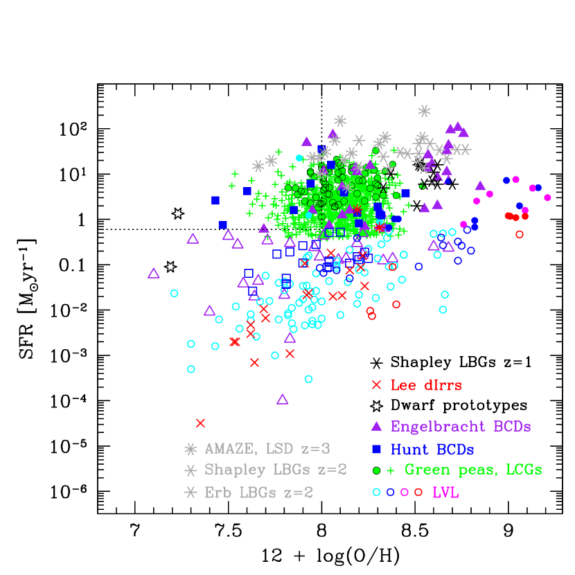
Figure 1: SFR plotted against nebular oxygen abundance. The LVL (11HUGS) galaxies are shown as small open or filled circles (filled when SFR$\geq$0.6 $M_{\odot}$ yr^-1), with different colors corresponding to Hubble type $T$ as in Lee et al. (2009): $T\geq$ 8 cyan, $5\leq T<8$ blue, $3\leq T<5$ magenta, and $T<3$ red. Red $\times$ corresponds to the dIrr sample; BCDs are shown as (blue) squares (Fumagalli$+$Hunt samples) and (purple) triangles (Engelbracht); Green Peas are given by small (green) filled circles; LCGs by $+$; LBGs at $z\sim 1$ (Shapley), $z\sim 2$ (Erb, Shapley) are shown as 6-pronged asterisks, and at $z\sim 3$ (Maiolino, Mannucci) as 8-pronged asterisks. 6-sided open stars show the two dwarf “prototypes”, SBS 0335$-$052 and I Zw 18. Solid symbols show those BCDs with SFR$\geq$0.6 $M_{\odot}$ yr^-1. The region in the upper left quadrant delineated by dotted lines corresponds to what we loosely define as a “low-metallicity starburst” (see text): SFR$\geq$0.6 $M_{\odot}$ yr^-1 and 12$+\log$(O/H)$\leq$8.0.

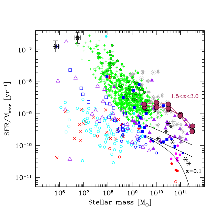
Figure 2: sSFR plotted against stellar mass, $M_{\rm star}$ (star-formation “Main Sequence”). Symbols are as in Fig. 1. The black curve and line correspond to the Local-Universe ($z=0.1$, Salim et al., 2007); the curve reproduces the best-fit Schecter function, and the line the best fit to “pure” (no AGN) star-forming galaxies. The black line with the higher normalization gives the intermediate-redshift trend ($0.2<z<0.7$, Noeske et al., 2007); and the bordeaux curves with round data points indicate the high-redshift relations ($1.5<z<3.0$, Bauer et al., 2011).

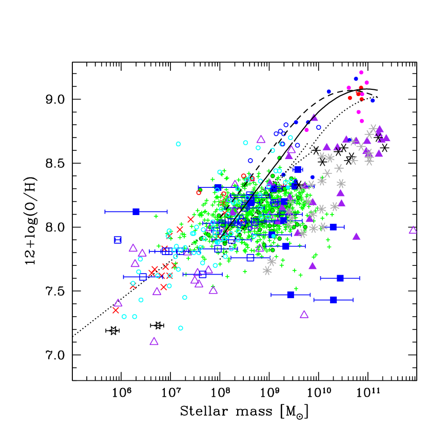
Figure 3: Nebular oxygen abundance, 12$+\log$(O/H), plotted against stellar mass, $M_{\rm star}$ (MZR, FMR). Symbols are as in Fig. 1. The black dotted line gives the linear relation found by Lee et al. (2006), and the curves correspond to the adjustments for SFR as advocated by Mannucci et al. (2011). SFRs consistent with the ranges considered by Mannucci et al. (2010, 2011) are shown (0.1 $M_{\odot}$ yr^-1, dashed line to the left; 1 $M_{\odot}$ yr^-1, solid line; 10 $M_{\odot}$ yr^-1, dotted line to the right).

Generally SFR increases with metallicity, although the correlation is far from perfect. Inspection of Fig. 1, which plots SFR against 12$+\log$(O/H), shows that in two of the local dwarf samples (LVL, dIrr) there is a clear increase of SFR with metallicity. The trend gets rather noisy for the BCD samples, and disappears completely for the LCG$+$Green Peas. Nevertheless, the statistical significance of the correlation of SFR with O/H over all the samples (1070 data points) is quite high, $\ga 10\,\sigma$. In fact, two regions tend to be underpopulated: the lower right quadrant with high abundances and low SFRs, and the upper left quadrant with low O/H and high SFRs. The galaxies that occupy this latter region are what we will call “low-metallicity starbursts”.

Figure 2 shows the “Star Formation Main Sequence” or SFMS. In addition to the data, three trends are shown as black curves extending only as far as the parameter space in the original samples they were derived from. The SFMS derived by Salim et al. (2007) for the Local Universe at $z\sim 0.1$ (both the linear relation and the “Schechter-like” curve) appears at lower sSFRs; the one proposed by Noeske et al. (2007) for galaxies at redshifts between 0.2 and 0.7 is roughly parallel to the previous one but with a larger offset; and the SFMS derived by Bauer et al. (2011) for a mass-selected sample between redshifts 1.5 and 3.0 has an even greater offset. The figure clearly shows that most of the AMAZE and LSD samples at $z\sim 3$ follow the Bauer et al. relation fairly well. However, the high-$z$ trend is also reflected in the LCGs and the Green Peas at $z\sim 0.3$, and several of the BCDs at $z\sim 0$. Most of the BCDs follow the Local Universe SFMS by Salim et al. (2007), but some galaxies at low stellar masses have excess SFR relative to the SFMS. At stellar masses $M_{\rm star}$$\sim 10^{8}$ $M_{\odot}$, the SFR of these outliers is $\ga 0.6$ $M_{\odot}$ yr^-1. This motivates our choice of SFR = 0.6 $M_{\odot}$ yr^-1 as a SFR threshold for starbursts at low metallicity. Such a low-mass galaxy would have an sSFR of $\sim 6\times 10^{-9}$ yr^-1, well outside the range probed by Salim et al. (2007), but roughly consistent with an extrapolation to lower masses of the “starburst sequence” they define.

The MZR for our data is shown in Figure 3. The FMR proposed by Mannucci et al. (2010) is also shown as a set of black curves; these curves are the predictions, based on the SDSS, of how SFR alters the MZR. The dashed curve corresponds to SFR = 0.1 $M_{\odot}$ yr^-1, i.e., where a galaxy with this SFR would lie relative to the MZR. The solid curve gives a correction for SFR = 1 $M_{\odot}$ yr^-1, and the dotted one SFR = 10 $M_{\odot}$ yr^-1; the curves span roughly the ranges in parameters of the Mannucci et al. (2010) sample. The FMR was subsequently extended to lower masses by Mannucci et al. (2011) (shown here as the linear extensions toward lower masses slightly detached from the main curved FMR). The linear MZR for low masses found by Lee et al. (2006) is also shown, but the slope with $M_{\rm star}$ is flatter ($\sim$0.3) than the slope found by Mannucci et al. (2011, $\sim$0.5).

Most of the AMAZE and LSD galaxies at $z\sim 3$ follow neither the MZR nor the FMR, and this was already noticed by Mannucci et al. (2010). However, some of the low-metallicity dwarf galaxies with SFR$\ga$0.6 $M_{\odot}$ yr^-1 are also outliers of both the MZR and the FMR, although galaxies with lower SFR follow the MZR and/or FMR quite well. The degree of deviation from the main trends increases for metal abundances at or below 12$+\log$(O/H)$\sim$8.0. Some metal-poor BCDs and high-$z$ LBGs in the AMAZE$+$LSD samples deviate from the MZR and FMR by factors of 100 or more in stellar mass. Hence, we adopt this abundance 12$+\log$(O/H) = 8.0 as a “fiducial location” in the MZR below which we can distinguish potential outliers; here we are interested in low-metallicity starbursts, and consequently concentrate on this metal-poor abundance regime and on high SFRs. The region delineated in Fig. 1 is occupied by these metal-poor starbursts, independently of their redshift. If a galaxy has 12$+\log$(O/H)$\leq$8.0 and SFR$\geq$0.6 $M_{\odot}$ yr^-1, we will call it a “low-metallicity starburst” (LMS).

3.1 Crude demographics

The only galaxy sample in our database which can be considered complete in any sense is the 11HUGS/LVL sample; it is approximately distance (thus volume) limited, and a fair representation of the nearby galaxy population. Of 113 galaxies in the LVL sample, only 2 (NGC 784 and NGC 4656) would be considered LMSs, a fraction of $\sim$ 2%. The fraction of low-metallicity starbursts in the BCD samples is 5 times higher, $\sim$11% (10 LMSs), but these galaxies have already been selected from the general galaxy population through the strength of their emission lines.

Among the LCGs and Green Peas, the fraction is higher still, but, again, these galaxies have been selected for strong emission lines; 176 galaxies out of 803 LCGs would be classified as a LMS, roughly 22%. This is partly a result of a selection effect because of the limit on H$\beta$ luminosity, and thus SFR, imposed by Izotov et al. (2011); all LCGs have SFRs greater than our fiducial cutoff by definition. At $z\sim 3$, there are 3 LMSs in the LSD sample of 9 and 2 LMSs of 9 AMAZE galaxies, or $\sim$27%; these are small-number statistics, but roughly consistent with the LCGs at a redshift 10 times smaller.

Outside the LVL and dIrr samples, virtually all the galaxies are selected on the basis of high equivalent widths in various emission lines. These samples have high LMS fractions, perhaps more similar to the LBGs at $z\sim 3$ than either the LVL or dIrr samples. This means that the differences in properties found for high-$z$ populations may result from differences in selection criteria, relative to the local galaxy populations. We may be observing locally a somewhat rare class of low-metallicity starbursts that are however similar to some high-$z$ galaxy populations such as LBGs. In the next section, we put this proposition on a firmer footing by showing the existence of a Fundamental Plane of O/H, SFR, and $M_{\rm star}$, which apparently does not vary with redshift.

4 The fundamental plane of metallicity, SFR, and stellar mass

Unlike the SDSS samples studied by other groups (Tremonti et al., 2004; Salim et al., 2007; Mannucci et al., 2010; Yates et al., 2012), our sample has been designed to probe low stellar masses, low metallicities, and (relatively) high SFRs. This makes it uniquely suited to exploring a much expanded parameter space, and the resulting scaling relations of metallicity, $M_{\rm star}$, and SFR. At high masses and metallicities, both the MZR and SFMS inflect and flatten. However, for $M_{\rm star}$$\leq 3\times 10^{10}$ $M_{\odot}$, roughly the “turn-over mass” (Tremonti et al., 2004; Wyder et al., 2007), the trends are very close to linear, independently of redshift. Hence, the observationally-defined variables (O/H, SFR, and $M_{\rm star}$) should define a plane which, given the relatively large scatters in the SFMS, the MZR, and the SFR-O/H relation, is not optimally viewed (see also Lara-López et al., 2010).

We can implicitly test the assumption that the relations among the observationally-defined variables are invariant, regardless of redshift. Hereafter, for brevity, we will call the “observationally-defined variables” observables, even though they are derived from observations rather than being directly observed. Like Mannucci et al. (2010), we propose that if the MZR and SFMS are observed to “evolve” or change with redshift, then this evolution or alteration must be due to different selection criteria for different galaxy populations at different lookback times. However, Mannucci et al. (2010) defined a “surface” by associating SFR with stellar mass, and plotting this combination against metallicity; they did not examine the mutual correlations among the three parameters. Metallicity, mass, and SFR are all correlated (see Sect. 3), but it is not clear which parameters are mainly responsible for the dispersion.

We have therefore performed a Principle Component Analysis (PCA) on all galaxies with stellar masses $\leq 3\times 10^{10}$ $M_{\odot}$ (1019 data points). A PCA diagonalizes the covariance matrix, thus giving the linear combinations of observables which define the orientations that minimize the covariance. These orientations are the eigenvectors and are, by definition, mutually orthogonal. In the 3-space formed by the three observables, to form a plane we would expect most of the variance to be contained in the first two eigenvectors; for the third, perpendicular, eigenvector the variance should be very small.

Our sample is particularly well suited for such an analysis; it spans almost two orders of magnitude in metallicity (12$+\log$(O/H) = 7.1 to $\sim 9$), a factor of $\sim 10^{6}$ in SFR ($\sim 10^{-4}\leq$ SFR $\leq\,\sim 10^{2}$ $M_{\odot}$ yr^-1), and a factor of $\sim 10^{5}$ in stellar mass ($\sim 10^{6}\leq$ $M_{\rm star}$ $\leq\,\sim 10^{11}$ $M_{\odot}$). Other samples previously analyzed to find scaling relations cover much smaller parameter ranges: typically less than a decade in metallicity (12$+\log$(O/H)$\geq$8.4), a factor of $\sim$200 in SFR ($\sim$0.04$\la$ SFR$\la 6$ $M_{\odot}$ yr^-1), and roughly 2 orders of magnitude in stellar mass ($M_{\rm star}$$\ga 10^{9}$ $M_{\odot}$) (e.g., Tremonti et al., 2004; Salim et al., 2007; Mannucci et al., 2010; Yates et al., 2012). This implies that our results should represent the extremes of SF processes, possibly closer to what is observed in the early universe than nearby. To avoid excessively weighting the LCGs, which effectively dominate our sample ($\sim$800/1000), we used a bootstrapping technique to randomly select a fraction of LCGs and repeat the PCA many times on different samples of $\sim$350-1000 objects.

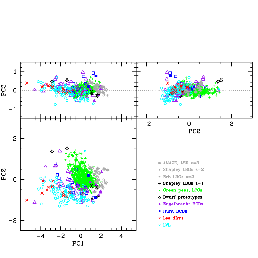
Figure 4: Different projections using the 3 PCs found by the PCA. Galaxies are coded as shown in the lower right (empty) panel. The top left and right panels show the orthogonal “edge-on” views of the plane; the bottom panel shows the plane face-on. $x_{1}\,=\,$12$+\log$(O/H)$-\langle$ 12$+\log$(O/H)$\rangle$, $x_{2}\,=\,\log(SFR)-\langle\log(SFR)\rangle$ ($M_{\odot}$ yr^-1), and $x_{3}\,=\,\log(M_{\rm star})-\langle\log(M_{\rm star})\rangle$ ($M_{\odot}$). $\langle$12$+\log$(O/H)$\rangle$ =  8.063; $\langle\log(SFR)\rangle$ =  $-0.594$; $\langle\log(M_{\rm star})\rangle$ = 8.476. PC1   =   0.12 $x_{1}$ + 0.75 $x_{2}$ + 0.65 $x_{3}$; PC2   =   -0.31 $x_{1}$ - 0.65 $x_{2}$ - 0.69 $x_{3}$; PC3   =   -0.94 $x_{1}$ - 0.11 $x_{2}$ + 0.31 $x_{3}$.

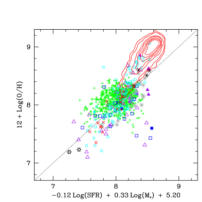
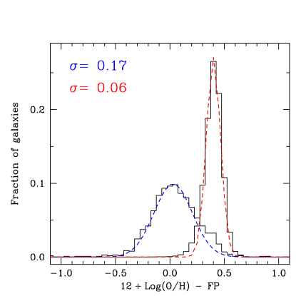
Figure 5: Left panel: the PC3 component shown as 12$+\log$(O/H) vs. the resulting linear combination of (log) SFR and $M_{\rm star}$ obtained from the PCA on our sample. Galaxies are coded as in Fig. 4. The FP applied to the FMR-SDSS sample is shown as red contours, with the innermost contour corresponding to 60% of the sample of 55 082 galaxies, and increasing to 70%, 80%, 90%, 95%, 99%, with 99.5% as the outermost contour. The dotted line in the left panel indicates equality. Right panel: the histogram of the residuals from the identity (dotted line) relation shown in the left panel; the blue Gaussian and broader distribution corresponds to our sample, and the red Gaussian and narrower distribution to the FMR-SDSS galaxies. The FMR-SDSS distribution is well fit by a Gaussian but offset by $+0.4$ dex. In both samples (and both panels), only galaxies with $M_{\rm star}$ $<10^{10.5}$ $M_{\odot}$ are shown.

The PCA shows that the set of three observables truly defines a plane; $\sim$97-98% of the total variance is contained in the first two eigenvectors. 80-85% (depending on the bootstrapping) of the variance is contained in the first eigenvector or Principle Component (PC), PC1; 12-17% of the variance is found in the second PC, PC2; and $\la$2-3% in PC3. Hence, the 3-space defined by O/H, SFR, and $M_{\rm star}$ is degenerate; only two independent parameters are necessary to describe the galaxies in these three dimensions.

The existence of a plane of O/H, SFR, and $M_{\rm star}$ for star-forming galaxies is not, however, a new result. Lara-López et al. (2010) found that a plane could describe a sample of $\sim$ 33 000 SDSS galaxies but, rather than performing a PCA, they fitted linear regressions to pairs of observables. They also included a second-order polynomial for low-metallicity mass bins, and concluded that a “linear combination of the metallicity and SFR as a function of stellar mass” could describe their sample. Thus, unlike Mannucci et al. (2010) who combined SFR and $M_{\rm star}$ to predict 12$+\log$(O/H), Lara-López et al. (2010) combined SFR with 12$+\log$(O/H) to predict $M_{\rm star}$, and find a dispersion $\sigma$ of 0.16 for the 33 000 SDSS galaxies in their sample.

For our sample, Fig. 4 shows three different projections of the plane defined by these three “basis” (eigen-) vectors that are different linear combinations of the observed variables:

$$PC1 = 0.12\,x_{1}+0.75\,x_{2}+0.65\,x_{3}$$ (1)

$$PC2 = -0.31\,x_{1}-0.65\,x_{2}-0.69\,x_{3}$$ (2)

$$PC3 = -0.94\,x_{1}-0.11\,x_{2}+0.31\,x_{3}$$ (3)

The PCA first normalizes the variables to zero mean, so that

$$x_{1} = 12+\log(O/H)-\langle 12+\log(O/H)\rangle$$

$$= 12+\log(O/H)-8.063$$

$$x_{2} = \log(SFR)-\langle\log(SFR)\rangle$$

$$= \log(SFR)+0.594\ \ M_{\odot}\,{\rm yr}^{-1}$$

$$x_{3} = \log(M_{\rm star})-\langle\log(M_{\rm star})\rangle$$

$$= \log M_{\rm star}-8.476\ \ M_{\odot}$$

The top panels of Fig. 4 show the best edge-on views of the plane, and the bottom panel its face-on view.

The first eigenvector PC1 is weighted roughly equally between SFR and $M_{\rm star}$; its dependence on O/H is relatively small. The same is true for PC2 with the relative weights between SFR and $M_{\rm star}$ reversed, but with a slightly increased dependence on O/H. This means that most of the dispersion in the 3-space is governed by the spreads in stellar mass and SFR, rather than by metallicity.

The eigenvector with the least variance, PC3, is dominated by metallicity with a secondary dependence on $M_{\rm star}$. Of the three parameters, metallicity is the least influential on the sample variance. Apparently, the plane is defined mainly by SFR and stellar mass $M_{\rm star}$ and its vertical extent or thickness by metallicity. However, this result may stem from the breadth and coverage of parameter space by our sample. In fact, our bootstrapping experiments suggest that the PCA coefficients depend slightly on the composition of the sample. The sample spread in SFR is particularly important as the SFR coefficients can change by 20-30%. Repeating a PCA on different samples would be worthwhile in order to gauge the generality of our results and the reliability of the coefficients (see below).

Since PC3 contains only $\sim$2% of the variation among the galaxies, it is a potentially powerful tool for establishing an optimized view of the parameter space defined by metallicity, stellar mass, and SFR. The tightness of PC3 and its dominant dependence on metallicity makes it possible to formulate a correlation between O/H, and some linear combination of the other two variables. The PCA has essentially distilled the information given by the MZR and the SFMS (and the trend of SFR with O/H), thus providing the combination of the relations with the lowest dispersion. If we take PC3 as shown in Fig. 4 and set it equal to zero, we can derive a best-fit relation among O/H, SFR, and $M_{\rm star}$, which is characterized by small variation over a wide range of parameter space. This is shown in the left panel in Figure 5 where we have plotted 12$+\log$(O/H) vs. the equation that results from equating PC3 to zero (only galaxies with $M_{\rm star}$$<3\times 10^{10}$ $M_{\odot}$ are shown).

$$12+\log(O/H)=-0.12\,{\rm log(SFR)}+0.33\,{\rm log(M_{\rm star})}+5.20\ \$$ (4)

The equality line in the left panel and the residuals in the right panel show that the observed abundance is well estimated by the FP. The reliability of this estimate is roughly constant over the entire parameter space covered by our sample; the errors shown in the right panel of Fig. 5 are well approximated by a Gaussian with a $\sigma\,=\,0.17$, or $\la$48-50% uncertainty (0.17 dex).

Also shown in Fig. 5 is the FP applied to the SDSS sample used to define the FMR (Mannucci et al., 2010); only galaxies with $M_{\rm star}$ $\leq 3\times 10^{10}$ $M_{\odot}$ are plotted. The dispersion of the SDSS sample around the FP defined here is small, $\sigma$ = 0.06 dex, the same as Mannucci et al. (2010) found relative to the FMR. However, the SDSS sample appears to be offset from the FP by $\sim$0.4 dex, as shown in the right panel of Fig. 5. The mean metallicity of the FMR-SDSS sample (with 55 082 galaxies having masses below $10^{10.5}$ $M_{\odot}$) is 8.94 ($\pm$0.14), roughly the limit of the maximum oxygen abundance in spiral galaxies (8.95: Pilyugin et al., 2007). Such metallicities are also well into the metallicity range known to have large discrepancies ($\lower 2.15277pt\hbox{$\;\buildrel>\over{\sim}\;$}0.4$ dex) relative to direct calibrations (e.g., Kewley & Ellison, 2008; Pilyugin et al., 2010). This is not a problem peculiar to the SDSS sample, since the metal-rich galaxies we examine here fall in a similar metallicity region (see Fig. 5).

As stated by Moustakas et al. (2010), “the factor of 5 absolute uncertainty in the nebular abundance scale poses one of the most important outstanding problems in observational astrophysics”. There is some evidence that calibrations based on theoretical strong-line calibrations (e.g., Tremonti et al., 2004; Kobulnicky & Kewley, 2004; Nagao et al., 2006) overestimate the nebular metallicity by 0.3$-$0.5 dex (e.g., Bresolin et al., 2009), but direct methods may underestimate it by 0.2$-$0.3 dex (e.g., Przybilla et al., 2008). Such discrepancies may be due to temperature mixing in the Hii regions in metal-rich giant spiral galaxies (e.g., Peimbert, 1967), but are much less common in metal-poor dwarfs (e.g., Pilyugin et al., 2010). In any case, different metallicity calibrations make comparing samples over wide ranges of abundances quite problematic, and are ultimately a major obstacle to probing scaling relations over a vast parameter space.

The FP fits the FMR-SDSS sample as well as the FMR itself ($\sigma\,=\,$0.06 dex), although with a $+0.4$ dex offset which could be due to problems with the metallicity calibration at high abundances (e.g., Bresolin et al., 2009). The FP dispersion of 0.17 dex for our sample(s) is higher than that found by Tremonti et al. (2004) for the MZR defined by 53 000 galaxies from the SDSS (0.1 dex), and also higher than the FMR (0.06 dex) found for the similar SDSS sample by Mannucci et al. (2011). However, both SDSS samples span limited ranges in O/H, SFR, and stellar mass relative to the parameter space covered by our sample. Indeed, the mean and standard deviation of (log) stellar mass for the FMR-SDSS sample (with $M_{\rm star}$$<10^{10.5}\,M_{\odot}$) is 10.07$\pm$0.31 (the comparable mean, standard deviation in our sample is 8.48$\pm$1.10). Thus, a lower dispersion in the fit is not surprising despite the many more galaxies in those samples. The value of the FP dispersion for the $\sim$1000 galaxies studied here is only slightly higher than that found for the MZR of 25 nearby dwarf galaxies (0.12 dex, Lee et al., 2006), another sample dominated by low-mass galaxies. Tremonti et al. (2004) and Mannucci et al. (2010) found that dispersion in the MZR increases with decreasing mass; hence given the parameter space covered by our sample, the $\sigma$ of 0.17 dex is reasonable.

It is also true that our sample is rather heterogeneous, in terms of the methods with which metallicity and stellar mass are calculated. Unfortunately this is of necessity since we are comparing properties of local and high-redshift galaxy populations, over a wide range of metallicity. Thus, it is possible that intrinsic systematics could be responsible for a fraction of the dispersion observed for our sample.

4.1 PCA of the SDSS sample

Because our original aim was to preferentially select metal-poor starbursts, our combined sample could be biased by metallicity. In such a case, the FP found here would not be applicable to general galaxy populations. To test this possibility, we performed a PCA of the SDSS sample used by Mannucci et al. (2010), considering only those galaxies (55 082) with $M_{\rm star}$$\leq 3\times 10^{10}$ $M_{\odot}$, the same limit as imposed for our sample. This is the same FMR-SDSS sample discussion in the previous section. If the coefficents and dispersions are similar to the ones obtained from the PCA on our sample, we could conclude that our sample is not unduly biased, and that the results can be generalized to broader galaxy populations.

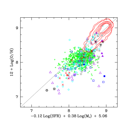
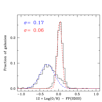
Figure 6: Left panel: the PC3 component shown as 12$+\log$(O/H) vs. the resulting linear combination of (log) SFR and $M_{\rm star}$ obtained from the PCA on the FMR-SDSS sample. Galaxies are coded as in Fig. 4. As in Fig. 5, the FMR-SDSS sample is shown as red contours, with the innermost contour corresponding to 60% of the sample of 55 082 galaxies, and increasing to 70%, 80%, 90%, 95%, 99%, with 99.5% as the outermost contour. The dotted line in the left panel indicates equality. Right panel: the histogram of the residuals from the identity (dotted line) relation shown in the left panel; the blue Gaussian and broader distribution corresponds to our sample, and the red Gaussian and narrower distribution to the FMR-SDSS galaxies. The distribution of residuals for our samples is well fit by a Gaussian but offset by $-0.3$ dex. In both samples (and both panels), only galaxies with $M_{\rm star}$ $<10^{10.5}$ $M_{\odot}$ are shown.

The eigenvectors resulting from the PCA on the FMR-SDSS are found to be very similar to those we obtained for our sample. Specifically, 98% of the variation among the parameters is contained in the first two eigenvectors, PC1 and PC2, and they are similarly dominated by $M_{\rm star}$ and SFR. Moreover, PC3, dominated by O/H, comprises only 2.3% of the variance. Thus, following the same reasoning as before, we have set PC3 equal to zero and solved for 12$+\log$(O/H). From the PCA on the 55 082 galaxies in the mass-limited FMR-SDSS, we find:

$$12+\log(O/H)=-0.12\,{\rm log(SFR)}+0.38\,{\rm log(M_{\rm star})}+5.06\ \$$ (5)

Comparison with Eq. 4 shows that the coefficient multiplying (log) SFR is the same as for our sample, but there is an offset of $-0.14$ in the constant. The $M_{\rm star}$ coefficient is also slightly steeper than for our sample (0.38 vs. 0.33), although not as steep as the 0.51 coefficient multiplying $M_{\rm star}$ in the extension of the FMR to low mass by Mannucci et al. (2011). The difference in the FP constants ($-0.14$) is not as large as the offset between the two samples ($-0.4$, see Fig. 5), but the larger coefficient multiplying (log) $M_{\rm star}$ compensates the difference. Fig. 6 shows both samples plotted with the FP defined by the FMR-SDSS galaxies, and the relative dispersions.

If we apply this new (SDSS) FP to our sample, we find the same spreads for both samples as with the original FP (0.17 dex, 0.06 dex, see Fig. 6). However, our sample requires an offset of $-0.3$ dex, slightly smaller (and of opposite sign as expected) than the SDSS offset relative to the original FP ($+0.4$ dex). Hence, the two formulations are probably equally good representations of galaxies up to $z\lower 2.15277pt\hbox{$\;\buildrel>\over{\sim}\;$}3$, across a wide range of stellar mass ($10^{6}<$$M_{\rm star}$$<3\times 10^{10}$ $M_{\odot}$), metallicity, and SFR ($10^{-4}<$SFR$<10^{2}$ $M_{\odot}$ yr^-1). Nevertheless, as discussed above, differences in metallicity calibrations make it difficult to accurately assess scaling relations across wide ranges of abundances.

4.2 Comparison with the FMR

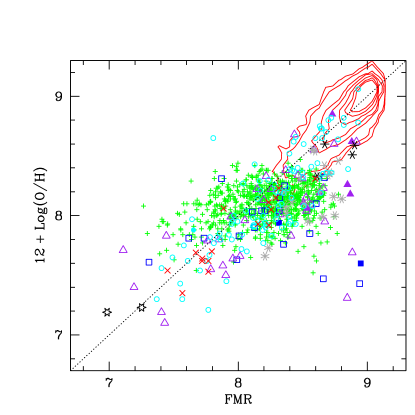
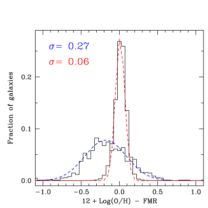
Figure 7: Left panel: nebular oxygen abundance, 12$+\log$(O/H), plotted against the FMR abscissas, as described in the text (there are two separate branches, according to the value of $\mu_{0.32}$, see Mannucci et al., 2011). Symbols and contours are as in Fig. 5; the dotted line indicates equality. Right panel: the histogram of the residuals from the identity (dotted line) relation shown in the left panel; the blue Gaussian and broader distribution corresponds to our sample, and the red Gaussian and narrower distribution to the FMR-SDSS galaxies. Our sample is offset by $-0.18$ dex, with a slightly asymmetric distribution. In both samples (and both panels), only galaxies with $M_{\rm star}$ $<10^{10.5}$ $M_{\odot}$ are shown; this mass limit is clearly evident in the left panel.

As mentioned in the Introduction, Mannucci et al. (2010) devised the Fundamental Metallicity Relation which significantly reduces the scatter in the MZR of SDSS-selected galaxies by introducing a dependence on the SFR. Mannucci et al. (2011) extended the FMR to lower masses ($\mu_{0.32}<9.5$) such that:

$$12+\log(O/H)=0.51(\mu_{0.32}-10)+8.93$$

$$\quad\quad\quad\quad=-0.16,{\rm log(SFR)}+0.51\,{\rm log(M_{\rm star})}+3.83\\$$ (6)

where $\mu_{0.32}$ = log(M_star)$-$0.32 log(SFR).

We have applied the FMR to our sample (considering also the non-linear extension to high masses) and find that the residuals have mean values of $\ga$0.32 dex, almost twice the value we find here for either FP. The FMR applied to our sample and to the FMR-SDSS sample is shown in Fig. 7. The residuals for our sample are asymmetrically skewed to negative values, and fitting them to a Gaussian gives $\sigma\,=\,0.27$ dex. Hence, the FMR is a poorer fit to our sample than the FP.

The reason is that the extension to lower masses proposed by Mannucci et al. (2011), with a slope of $0.51$, is too steep to fit the galaxies in our sample (see also Fig. 1). From the PCA, we find a metallicity-mass dependence of 0.33, similar to Lee et al. (2006) who found for their low-mass dIrr sample a linear dependence (in log-log) of 0.30 between 12$+\log$(O/H) and $M_{\rm star}$ ($\sigma\,=\,$0.12 dex). This shallower dependence of metallicity on mass may be peculiar to samples with many low-mass galaxies, although we find similar values even when restricting the fits to only the highest masses, and when fitting the FMR-SDSS sample.

Nevertheless, the relative dependence between $M_{\rm star}$ and SFR found by our PCA is similar to that given by Mannucci et al. (2010). With $\mu_{0.32}$, they assumed a unit dependence of O/H on (log)$M_{\rm star}$, and found that the value of 0.32 multiplying (log)SFR minimizes the residuals of the MZR relative to $\mu$. The extension to lower masses by Mannucci et al. (2011) has a flatter dependence of O/H on $\mu_{0.32}$, 0.51 (see above), but the same value of 0.32 relating (log)SFR to $M_{\rm star}$. For the FP, we find a shallower dependence of O/H on $M_{\rm star}$ (0.33), and a SFR coefficient of $-0.12$; multiplying 0.33 (our mass dependence) by the 0.32 SFR factor of Mannucci et al. (2010) would give a SFR dependence of $-0.11$, very similar to the value of $-0.12$ given by the PCA.

5 Discussion and conclusions

From a sample of $\sim 1100$ galaxies spanning a wide range of O/H, SFR, and $M_{\rm star}$, we have identified a class of low-metallicity starbursts which deviate from the SFMS and the MZR in the same way, independently of redshift. When these scaling relations are considered together, the sample as a whole (although excluding the galaxies with $M_{\rm star}$$>3\times 10^{10}$ $M_{\odot}$) defines a Fundamental Plane whose orientation is defined primarily by SFR and $M_{\rm star}$, and whose thickness is governed by O/H.

The two-dimensional nature of the plane in the 3-space defined by the observables implies that only two parameters are necessary to describe a galaxy (see also Lara-López et al., 2010). The thinness of the plane when viewed edge-on enables the formulation of a relation which combines the SFMS and the MZR in an optimal way. Through application of a PCA, we have established a dependence of O/H on SFR and $M_{\rm star}$ which has a deviation over the whole sample (for $M_{\rm star}$$\leq 3\times 10^{10}$ $M_{\odot}$) of 0.17 dex, or $\sim$48%.

The FP from the PCA applied to the SDSS sample used to define the FMR (Mannucci et al., 2010) is similar to that obtained for our sample (see Eqs. 4, 5). Applying either FP to our sample and to the FMR-SDSS shows an offset in metallicity which distinguishes the two, but the dispersions are similarly low (0.17 dex and 0.06 dex for our and the FMR-SDSS samples, respectively). However, the FMR is not the best description of our sample, as it gives a higher dispersion (0.27 dex) than either FP.

Perhaps the most intriguing aspect of the FPs given by the PCA is that they hold for all the redshifts we have examined, $z\la 3$. In our sample, the LBGs at all redshifts follow the “Fundamental Plane” relation which combines the MZR and the SFMS. There are no high-redshift outliers. Moreover, the low-metallicity starbursts at all redshifts also follow the relation. On the basis of O/H, SFR, and stellar mass alone, apparently there is no distinction between the behavior of galaxies in the Local Universe and those at high redshift (at least up to $\la 3$).

The statistical analysis does not clarify which relation or which observable is the most important; it merely indicates that there is a plane that describes the family of galaxies in the 3-space of O/H, SFR, and $M_{\rm star}$. However, the small amount of variance contained in the eigenvector dominated by metallicity (PC3) suggests that metallicity is the least important of the three parameters in driving the variance of our sample. The physics of why or how these parameters conspire to form a plane independent of redshift will be explored in a companion paper (Magrini et al., 2012). There we show that the deviations from the main scaling relations are due to a different mode of star formation, a starburst or “active” mode which evolves over relatively short timescales. The main scaling relations are instead defined by a more quiescent, “passive” mode of star formation which evolves more slowly.

The existence of a Fundamental Plane that spans redshifts up to $z\ga 3$ implies that the SFMS and MZR do not really change with lookback time, but rather that the galaxy populations that define them change with redshift. Starbursts become increasingly common at high redshift, but they also exist locally and at low metallicity. Thus, the “evolution” in the scaling relations is a result of selecting those galaxies which are most common at a particular redshift, and may not reflect a true change in the physics of how galaxies evolve.

References

- Amorín et al. (2010) Amorín, R. O., Pérez-Montero, E., & Vílchez, J. M. 2010, ApJL, 715, L128
- Atek et al. (2011) Atek, H., Siana, B., Scarlata, C., et al. 2011, ApJ, 743, 121
- Bauer et al. (2011) Bauer, A. E., Conselice, C. J., Pérez-González, P. G., et al. 2011, MNRAS, 417, 289
- Bell & de Jong (2001) Bell, E. F., & de Jong, R. S. 2001, ApJ, 550, 212
- Boselli et al. (2009) Boselli, A., Boissier, S., Cortese, L., et al. 2009, ApJ, 706, 1527
- Bothwell et al. (2009) Bothwell, M. S., Kennicutt, R. C., & Lee, J. C. 2009, MNRAS, 400, 154
- Bresolin et al. (2009) Bresolin, F., Gieren, W., Kudritzki, R.-P., et al. 2009, ApJ, 700, 309
- Bruzual & Charlot (2003) Bruzual, G., & Charlot, S. 2003, MNRAS, 344, 1000
- Cardamone et al. (2009) Cardamone, C., Schawinski, K., Sarzi, M., et al. 2009, MNRAS, 399, 1191
- Chabrier (2003) Chabrier, G. 2003, PASP, 115, 763
- Dale et al. (2009) Dale, D. A., Cohen, S. A., Johnson, L. C., et al. 2009, ApJ, 703, 517
- Draine & Li (2007) Draine, B. T., & Li, A. 2007, ApJ, 657, 810
- Engelbracht et al. (2008) Engelbracht, C. W., Rieke, G. H., Gordon, K. D., et al. 2008, ApJ, 678, 804
- Erb et al. (2006) Erb, D. K., Shapley, A. E., Pettini, M., et al. 2006, ApJ, 644, 813
- Fontana et al. (2006) Fontana, A., Salimbeni, S., Grazian, A., et al. 2006, A&A, 459, 745
- Fumagalli et al. (2010) Fumagalli, M., Krumholz, M. R., & Hunt, L. K. 2010, ApJ, 722, 919
- Gavazzi (1993) Gavazzi, G. 1993, ApJ, 419, 469
- Gil de Paz et al. (2003) Gil de Paz, A., Madore, B. F., & Pevunova, O. 2003, ApJS, 147, 29
- Guseva et al. (2006) Guseva, N. G., Izotov, Y. I., & Thuan, T. X. 2006, ApJ, 644, 890
- Helou et al. (2004) Helou, G., Roussel, H., Appleton, P., et al. 2004, ApJS, 154, 253
- Hirashita & Hunt (2004) Hirashita, H., & Hunt, L. K. 2004, A&A, 421, 555
- Hoyos et al. (2005) Hoyos, C., Koo, D. C., Phillips, A. C., Willmer, C. N. A., & Guhathakurta, P. 2005, ApJL, 635, L21
- Hunt et al. (2005) Hunt, L. K., Dyer, K. K., & Thuan, T. X. 2005, A&A, 436, 837
- Hunt et al. (2002) Hunt, L. K., Giovanardi, C., & Helou, G. 2002, A&A, 394, 873
- Hunt & Hirashita (2009) Hunt, L. K., & Hirashita, H. 2009, A&A, 507, 1327
- Hunt et al. (2010) Hunt, L. K., Thuan, T. X., Izotov, Y. I., & Sauvage, M. 2010, ApJ, 712, 164
- Hunt et al. (2001) Hunt, L. K., Vanzi, L., & Thuan, T. X. 2001, A&A, 377, 66
- Izotov et al. (2007) Izotov, Y. I., Thuan, T. X., & Stasińska, G. 2007, ApJ, 662, 15
- Izotov et al. (2011) Izotov, Y. I., Guseva, N. G., & Thuan, T. X. 2011, ApJ, 728, 161
- Jun & Im (2008) Jun, H. D., & Im, M. 2008, ApJL, 678, L97
- Kennicutt (1998) Kennicutt, R. C., Jr. 1998, ARA&A, 36, 189
- Kennicutt et al. (2008) Kennicutt, R. C., Jr., Lee, J. C., Funes, S. J., José G., Sakai, S., & Akiyama, S. 2008, ApJS, 178, 247
- Kewley & Ellison (2008) Kewley, L. J., & Ellison, S. L. 2008, ApJ, 681, 1183
- Kobulnicky & Kewley (2004) Kobulnicky, H. A., & Kewley, L. J. 2004, ApJ, 617, 240
- Lara-López et al. (2010) Lara-López, M. A., Cepa, J., Bongiovanni, A., et al. 2010, A&A, 521, L53
- Lee et al. (2006) Lee, H., Skillman, E. D., Cannon, J. M., et al. 2006, ApJ, 647, 970
- Lee et al. (2011) Lee, J. C., Gil de Paz, A., Kennicutt, R. C., Jr., et al. 2011, ApJS, 192, 6
- Lee et al. (2009) Lee, J. C., Gil de Paz, A., Tremonti, C., et al. 2009, ApJ, 706, 599
- Lee et al. (2007) Lee, J. C., Kennicutt, R. C., Funes, S. J., José G., Sakai, S., & Akiyama, S. 2007, ApJL, 671, L113
- Lee et al. (2004) Lee, J. C., Salzer, J. J., & Melbourne, J. 2004, ApJ, 616, 752
- Magrini et al. (2012) Magrini, L., Galli, D., Hunt, L., Schneider, Bianchi, S., Maiolino, R., Romano, D., Tosi, M., Valiante, R. 2012, MNRAS, submitted
- Maiolino et al. (2008) Maiolino, R., Nagao, T., Grazian, A., et al. 2008, A&A, 488, 463
- Mannucci et al. (2009) Mannucci, F., Cresci, G., Maiolino, R., et al. 2009, MNRAS, 398, 1915
- Mannucci et al. (2010) Mannucci, F., Cresci, G., Maiolino, R., Marconi, A., & Gnerucci, A. 2010, MNRAS, 408, 2115
- Mannucci et al. (2011) Mannucci, F., Salvaterra, R., & Campisi, M. A. 2011, MNRAS, 414, 1263
- Marble et al. (2010) Marble, A. R., Engelbracht, C. W., van Zee, L., et al. 2010, ApJ, 715, 506
- McGaugh (1991) McGaugh, S. S. 1991, ApJ, 380, 140
- Melena et al. (2009) Melena, N. W., Elmegreen, B. G., Hunter, D. A., & Zernow, L. 2009, AJ, 138, 1203
- Moustakas et al. (2010) Moustakas, J., Kennicutt, R. C., Jr., Tremonti, C. A., et al. 2010, ApJS, 190, 233
- Nagao et al. (2006) Nagao, T., Maiolino, R., & Marconi, A. 2006, A&A, 459, 85
- Noeske et al. (2007) Noeske, K. G., Weiner, B. J., Faber, S. M., et al. 2007, ApJL, 660, L43
- Osterbrock & Ferland (2006) Osterbrock, D. E., & Ferland, G. J. 2006, Astrophysics of gaseous nebulae and active galactic nuclei, 2nd. ed. by D.E. Osterbrock and G.J. Ferland. Sausalito, CA: University Science Books, 2006
- Peeples et al. (2009) Peeples, M. S., Pogge, R. W., & Stanek, K. Z. 2009, ApJ, 695, 259
- Peimbert (1967) Peimbert, M. 1967, ApJ, 150, 825
- Pérez-González et al. (2008) Pérez-González, P. G., Rieke, G. H., Villar, V., et al. 2008, ApJ, 675, 234
- Pilyugin et al. (2007) Pilyugin, L. S., Thuan, T. X., & Vílchez, J. M. 2007, MNRAS, 376, 353
- Pilyugin et al. (2010) Pilyugin, L. S., Vílchez, J. M., & Thuan, T. X. 2010, ApJ, 720, 1738
- Pozzetti et al. (2007) Pozzetti, L., Bolzonella, M., Lamareille, F., et al. 2007, A&A, 474, 443
- Przybilla et al. (2008) Przybilla, N., Nieva, M.-F., & Butler, K. 2008, ApJL, 688, L103
- Reines et al. (2010) Reines, A. E., Nidever, D. L., Whelan, D. G., & Johnson, K. E. 2010, ApJ, 708, 26
- Rosario et al. (2008) Rosario, D. J., Hoyos, C., Koo, D., & Phillips, A. 2008, IAU Symposium, 255, 397
- Rodighiero et al. (2010) Rodighiero, G., Cimatti, A., Gruppioni, C., et al. 2010, A&A, 518, L25
- Rodighiero et al. (2011) Rodighiero, G., Daddi, E., Baronchelli, I., et al. 2011, ApJL, 739, L40
- Salim et al. (2007) Salim, S., Rich, R. M., Charlot, S., et al. 2007, ApJS, 173, 267
- Salpeter (1955) Salpeter, E. E. 1955, ApJ, 121, 161
- Salzer et al. (2009) Salzer, J. J., Williams, A. L., & Gronwall, C. 2009, ApJL, 695, L67
- Savaglio et al. (2005) Savaglio, S., Glazebrook, K., Le Borgne, D., et al. 2005, ApJ, 635, 260
- Schiminovich et al. (2007) Schiminovich, D., Wyder, T. K., Martin, D. C., et al. 2007, ApJS, 173, 315
- Shapley et al. (2005a) Shapley, A. E., Coil, A. L., Ma, C.-P., & Bundy, K. 2005a, ApJ, 635, 1006
- Shapley et al. (2004) Shapley, A. E., Erb, D. K., Pettini, M., Steidel, C. C., & Adelberger, K. L. 2004, ApJ, 612, 108
- Smith & Hancock (2009) Smith, B. J., & Hancock, M. 2009, AJ, 138, 130
- Steidel et al. (2003) Steidel, C. C., Adelberger, K. L., Shapley, A. E., et al. 2003, ApJ, 592, 728
- Steidel et al. (2004) Steidel, C. C., Shapley, A. E., Pettini, M., et al. 2004, ApJ, 604, 534
- Thuan & Martin (1981) Thuan, T. X., & Martin, G. E. 1981, ApJ, 247, 823
- Tolstoy et al. (2009) Tolstoy, E., Hill, V., & Tosi, M. 2009, ARA&A, 47, 371
- Tremonti et al. (2004) Tremonti, C. A., Heckman, T. M., Kauffmann, G., et al. 2004, ApJ, 613, 898
- Weisz et al. (2011) Weisz, D. R., Dalcanton, J. J., Williams, B. F., et al. 2011, ApJ, 739, 5
- Woo et al. (2008) Woo, J., Courteau, S., & Dekel, A. 2008, MNRAS, 390, 1453
- Wyder et al. (2007) Wyder, T. K., Martin, D. C., Schiminovich, D., et al. 2007, ApJS, 173, 293
- Yates et al. (2012) Yates, R. M., Kauffmann, G., & Guo, Q. 2012, MNRAS, 2572
- Zahid et al. (2012) Zahid, H. J., Bresolin, F., Kewley, L. J., Coil, A. L., & Davé, R. 2012, ApJ, 750, 120
- Zheng et al. (2007) Zheng, X. Z., Bell, E. F., Papovich, C., et al. 2007, ApJL, 661, L41