A Max-Product EM Algorithm for
Reconstructing Markov-tree Sparse Signals
from Compressive Samples

Abstract

We propose a Bayesian expectation-maximization (em) algorithm for reconstructing Markov-tree sparse signals via belief propagation. The measurements follow an underdetermined linear model where the regression-coefficient vector is the sum of an unknown approximately sparse signal and a zero-mean white Gaussian noise with an unknown variance. The signal is composed of large- and small-magnitude components identified by binary state variables whose probabilistic dependence structure is described by a Markov tree. Gaussian priors are assigned to the signal coefficients given their state variables and the Jeffreys’ noninformative prior is assigned to the noise variance. Our signal reconstruction scheme is based on an em iteration that aims at maximizing the posterior distribution of the signal and its state variables given the noise variance. We construct the missing data for the em iteration so that the complete-data posterior distribution corresponds to a hidden Markov tree (hmt) probabilistic graphical model that contains no loops and implement its maximization (m) step via a max-product algorithm. This em algorithm estimates the vector of state variables as well as solves iteratively a linear system of equations to obtain the corresponding signal estimate. We select the noise variance so that the corresponding estimated signal and state variables obtained upon convergence of the em iteration have the largest marginal posterior distribution. We compare the proposed and existing state-of-the-art reconstruction methods via signal and image reconstruction experiments.

I INTRODUCTION

The advent of compressive sampling (compressed sensing) in the past few years has sparked research activity in sparse signal reconstruction, whose main goal is to estimate the sparsest $p\times 1$ signal coefficient vector $\boldsymbol{s}$ from the $N\times 1$ measurement vector $y$ satisfying the following underdetermined system of linear equations:

$$\boldsymbol{y}=H\boldsymbol{s}$$ (1)

where $H$ is an $N\times p$ sensing matrix and $N\leq p$.

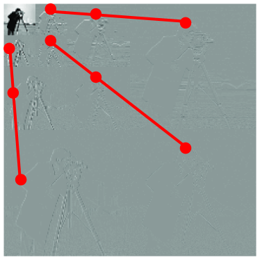
A tree dependency structure is exhibited by the wavelet coefficients of many natural images [1, 2, 3, 4, 5, 6, 7] (see also Fig. 1 and [3, Fig. 2]) as well as one-dimensional signals [1, 8, 7]. A probabilistic Markov tree structure has been introduced in [1] to model the statistical dependency between the state variables of wavelet coefficients. An approximate belief propagation algorithm has been first applied to compressive sampling by Baron, Sarvotham, and Baraniuk in [9], which employs sparse Rademacher sensing matrices for Bayesian signal reconstruction. Donoho, Maleki, and Montanari [10] simplified the sum-product algorithm by approximating messages using a Gaussian distribution specified by two scalar parameters, leading to their approximate message passing approximate message passing (amp) algorithm. Following the amp framework, Schniter [11] proposed a turbo-amp structured sparse signal recovery method based on loopy belief propagation and turbo equalization and applied it to reconstruct one-dimensional signals; [6] applied the turbo-amp approach to reconstruct compressible images. A generalized approximate message passing (gamp) algorithm that generalizes the amp algorithm to arbitrary input and output channels and incorporates both max-sum and sum-product loopy belief propagation separately is proposed in [12]. However, the above references do not employ the exact form of the messages and also have the following limitations: [9] relies on sparsity of the sensing matrix, the methods in [9, 10, 12] apply to unstructured signals only, and the turbo-amp approach in [6] and [11] needs sensing matrices to have approximately independent, identically distributed (i.i.d.) elements, see [6, Section. III-C]. Indeed, turbo-amp is sensitive to the presence of correlations among the elements of the sampling matrix and performs poorly if these correlations are sufficiently high and if norms of the columns or rows of the sampling matrix are sufficiently variable.

In [4] and [5], Markov chain Monte Carlo (mcmc) and variational Bayesian (vb) schemes are used to reconstruct images that follow probabilistic Markov tree structure from linear measurements; however, [4] and [5] did not report large-scale examples: these schemes are computationaly demanding and do not scale with increasing dimensionality of the reconstruction problem.

In this paper, we combine the hierarchical measurement model in [13] with a Markov tree prior on the binary state variables that identify the large- and small-magnitude signal coefficients and develop a Bayesian maximum a posteriori (map) expectation-maximization (em) signal reconstruction scheme that aims at maximizing the posterior distribution of the signal and its state variables given the noise variance, where the maximization (m) step employs a max-product belief propagation algorithm. Unlike the turbo-amp scheme in [6] and [11], our reconstruction scheme does not require sensing matrices to have approximately i.i.d. elements and can handle correlations among these elements. Unlike the previous work, we do not approximate the message form in our belief propagation scheme. Indeed, the m step of our em algorithm is exact because the expected complete-data posterior distribution that we maximize in the m step corresponds to the hidden Markov tree (hmt) graphical model that contains no loops. In [14], we proposed a similar em algorithm for a random signal model [15] with a purely sparse vector of signal coefficients and a noninformative prior on this component given the binary state variables. We apply a grid search to select the noise variance so that the estimated signal and state variables have the largest marginal posterior distribution.

In Section II, we introduce our measurement and prior models. We assume that the Markov tree prior distribution is known. To reduce the number of tuning parameters for the tree prior, we further assume that these parameters do not change between Markov tree levels. This is in contrast to other approaches (e.g., [4], [6], and [5]), which learn the Markov tree parameters from the measurements and allow their variation across the tree levels, see also the discussions in Sections V-B2 and VI. Section III describes the proposed em algorithm and establishes its properties; the implementation of the m step via the max-product algorithm is presented in Section III-A. The selection of the noise variance parameter is discussed in Section IV. Numerical simulations in Section V compare reconstruction performances of the proposed and existing methods.

We introduce the notation: $I_{n}$ and $\mathbf{0}_{n\times 1}$ denote the identity matrix of size $n$ and the $n\times 1$ vector of zeros, respectively; “^T”, $\det(\cdot)$, and $\left\|\cdot\right\|_{p}$ are the transpose, determinant, and $\ell_{p}$ norm, respectively; $\mathcal{N}(\mbox{\boldmath$x$}|\mbox{\boldmath$\mu$},\Sigma)$ denotes the probability density function (pdf) of a multivariate Gaussian random vector $x$ with mean $\mu$ and covariance matrix $\Sigma$; $\operatorname{Inv-\chi^{2}}2(\sigma^{2}|\nu,\sigma_{0}^{2})$ denotes the pdf of a scaled inverse chi-square distribution with $\nu$ degrees of freedom and a scale parameter $\sigma_{0}^{2}$, see [16, App. A]; $\mathbbm{D}\mathinner{\bigl{(}p(\boldsymbol{x})\,\|\,q(\boldsymbol{x})\bigr{)}}$ denotes the Kullback-Leibler (kl) divergence from pdf $p(\boldsymbol{x})$ to pdf $q(\boldsymbol{x})$ [17, Sec. 2.8.2], [18, Sec. 8.5]; $|\mathcal{T}|$ is the cardinality of the set $\mathcal{T}$; $\upsilon(\cdot)$ is an invertible operator that transforms the two-dimensional matrix element indices into one-dimensional vector element indices. Finally, $\rho_{H}$ denotes the largest singular value of a matrix $H$, also known as the spectral norm of $H$, and “$\odot$” denotes the Hadamard (elementwise) product.

II Measurement and Prior Models

We model an $N\times 1$ real-valued measurement vector $y$ using the standard additive white Gaussian noise measurement model with the likelihood function given by the following pdf [3, 6]:

$$p_{\boldsymbol{y}|\boldsymbol{s},\sigma^{2}}(\boldsymbol{y}|\boldsymbol{s},\sigma^{2})=\mathcal{N}(\boldsymbol{y}|H\boldsymbol{s},\sigma^{2}I_{N})$$ (2)

where $H$ is an $N\times p$ real-valued sensing matrix with $\operatorname{rank}(H)=N$ satisfying the spectral norm condition

$$\rho_{H}=1$$ (3)

$\boldsymbol{s}=[s_{1},s_{2},\ldots,s_{p}]^{T}$ is an unknown $p\times 1$ real-valued signal coefficient vector, and $\sigma^{2}$ is the unknown noise variance. We assume (3) without loss of generality because it is easily satisfied by appropriate scaling of the sensing matrix, measurements, and noise variance, provided that the spectral norm of the sensing matrix is easy to determine, see also footnote 2 for comments on the case where the spectral norm of the sensing matrix cannot be easily determined or estimated.

We adopt the Jeffreys’ noninformative prior for the variance component $\sigma^{2}$:

$$p_{\sigma^{2}}(\sigma^{2})\propto(\sigma^{2})^{-1}.$$ (4)

Define the vector of binary state variables $\mbox{\boldmath$q$}=[q_{1},q_{2},\dotsc,q_{p}]^{T}\in\{0,1\}^{p}$ that determine if the magnitudes of the signal components $s_{i},\,i=1,2,\ldots,p$ are small ($q_{i}=0$) or large ($q_{i}=1$). Assume that $s_{i}$ are conditionally independent given $q_{i}$ and assign the following prior pdf to the signal coefficients:

$$p_{\boldsymbol{s}|\boldsymbol{q},\sigma^{2}}(\boldsymbol{s}|\boldsymbol{q},\sigma^{2})=\prod_{i=1}^{p} [\mathcal{N}(s_{i}|0,\gamma^{2}\sigma^{2})]^{q_{i}}[\mathcal{N}(s_{i}|0,\epsilon^{2}\sigma^{2})]^{1-q_{i}}$$ (5a)

where $$\gamma^{2} \epsilon^{2} \gamma^{2}\gg\epsilon^{2} s_{i} q_{i}=1 q_{i}=0 \gamma^{2}\sigma^{2} \epsilon^{2}\sigma^{2} \gamma^{2} \epsilon^{2} \sigma^{2}$$ and are known positive constants and, typically, . Hence, the large- and small-magnitude signal coefficients corresponding to and are modeled as zero-mean Gaussian random variables with variances and , respectively. Consequently, and are relative variances (to the noise variance ) of the large- and small-magnitude signal coefficients. Equivalently,

$$p_{\boldsymbol{s}|\boldsymbol{q},\sigma^{2}}(\boldsymbol{s}|\boldsymbol{q},\sigma^{2})=\mathcal{N}(\boldsymbol{s}|\mathbf{0}_{p\times 1},\sigma^{2}D(\boldsymbol{q}))$$ (5b)

where

$$D(\mbox{\boldmath$q$})=\operatorname{diag}\bigl{\{}(\gamma^{2})^{q_{1}}(\epsilon^{2})^{1-q_{1}},(\gamma^{2})^{q_{2}}(\epsilon^{2})^{1-q_{2}},\dotsc,(\gamma^{2})^{q_{p}}(\epsilon^{2})^{1-q_{p}}\bigr{\}}.$$ (5c)

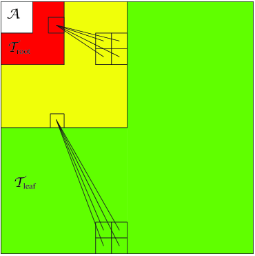
We now introduce the Markov tree prior probability mass function (pmf) on the state variables $q_{i}$ [1, 6]. To make this probability model easier to understand, we focus on the image reconstruction scenario where the elements of $\boldsymbol{s}$ are the two-dimensional discrete wavelet transform (dwt) coefficients of the underlying image that we wish to reconstruct. Hence, we introduce two-dimensional signal element indices $(i_{1},i_{2})$. Recall that the conversion operator $\upsilon(\cdot)$ is invertible; hence, there is a one-to-one correspondence between the corresponding one- and two-dimensional signal element indices. A parent wavelet coefficient with a two-dimensional position index $(i_{1},i_{2})$ has four children in the finer wavelet decomposition level with two-dimensional indices $(2i_{1}-1,2i_{2}-1)$, $(2i_{1}-1,2i_{2})$, $(2i_{1},2i_{2}-1)$ and $(2i_{1},2i_{2})$, see Fig. 1. The parent-child dependency assumption implies that, if a parent coefficient in a certain wavelet decomposition level has small (large) magnitude, then its children coefficients in the next finer wavelet decomposition level tend to have small (large) magnitude as well. Denote by $\rho$ and $\kappa$ the numbers of rows and columns of the image, and by $L$ the number of wavelet decomposition levels (tree depth).

Figure 1: (a) Clustering of significant discrete wavelet transform coefficients of a compressed ‘Cameraman’ image and (b) types of wavelet decomposition coefficients: approximation, root, and leaf, whose sets are denoted by $\mathcal{A},\mathcal{T}_{\textup{root}}$, and $\mathcal{T}_{{\scriptstyle{\rm leaf}}}$, respectively.

We set the prior pmf $p_{\boldsymbol{q}}(\boldsymbol{q})$ as follows. In the first wavelet decomposition level ($l=1$), assign

$$p_{q_{i}}(1)=\operatorname{Pr}\{q_{i}=1\}=\begin{cases}1,&i\in\mathcal{A}\\ P_{\textup{root}},&i\in\mathcal{T}_{\textup{root}}\end{cases}$$ (6a)

where

$$\mathcal{A} = \upsilon\Bigl{(}\Bigl{\{}1,2,\dotsc,\frac{\rho}{2^{L}}\Bigr{\}}\times\Bigl{\{}1,2,\ldots,\frac{\kappa}{2^{L}}\Bigr{\}}\Bigr{)}$$ (6b)

$$\mathcal{T}_{\textup{root}} = \upsilon\Bigl{(}\Bigl{\{}1,2,\dotsc,\frac{\rho}{2^{L-1}}\Bigr{\}}\times\Bigl{\{}1,2,\dotsc,\frac{\kappa}{2^{L-1}}\Bigr{\}}\Bigr{)}\,\big{\backslash}\,\mathcal{A}$$ (6c)

are the sets of indices of the approximation and root node coefficients and $$P_{\textup{root}}\in(0,1) l=2,3,\ldots,L$$ is a known constant denoting the prior probability that a root node signal coefficient has large magnitude, see Fig. 1. In the levels , assign

$$p_{q_{i}|q_{\pi(i)}}(1|q_{\pi(i)})=\begin{cases}P_{\textup{H}},&q_{\pi(i)}=1\\ P_{\textup{L}},&q_{\pi(i)}=0\end{cases}$$ (6d)

where $\pi(i)$ denotes the index of the parent of node $i$. Here, $P_{\textup{H}}\in(0,1)$ and $P_{\textup{L}}\in(0,1)$ are known constants denoting the probabilities that the signal coefficient $s_{i}$ is large if the corresponding parent signal coefficient is large or small, respectively.

The expected number of large-magnitude signal coefficients is

$$\operatorname{E}\biggl{[}\sum_{i=1}^{p}q_{i}\biggr{]}=\frac{p}{4^{L}}\biggl{(}1+3\sum_{l=0}^{L-1}4^{l}P_{l}\biggr{)}$$ (7a)

where $$P_{l} l$$ is the marginal probability that a state variable in the th tree level is equal to one, computed recursively as follows:

$$P_{l}=P_{l-1}P_{\textup{H}}+(1-P_{l-1})P_{\textup{L}}$$ (7b)

initialized by $P_{0}=P_{\textup{root}}$.

Our wavelet tree structure consists of $|\mathcal{T}_{\textup{root}}|$ trees and spans all signal wavelet coefficients except the approximation coefficients; hence, the set of indices of the wavelet coefficients within the trees is

$$\mathcal{T}=\upsilon\bigl{(}\{1,2,\ldots,\rho\}\times\{1,2,\ldots,\kappa\}\bigr{)}\,\backslash\,\mathcal{A}.$$ (8a)

Define also the set of leaf variable node indices within the tree structure as

$$\mathcal{T}_{{\scriptstyle{\rm leaf}}} = \upsilon\Bigl{(}\bigl{[}\{1,2,\ldots,\rho\}\times\{1,2,\ldots,\kappa\}\bigr{]}\,\big{\backslash}\,\Bigl{[}\Bigl{\{}1,2,\dotsc,\frac{\rho}{2}\Bigr{\}}\times\Bigl{\{}1,2,\dotsc,\frac{\kappa}{2}\Bigr{\}}\Bigr{]}\Bigr{)}$$ (8b)

see Fig. 1.

We have $5$ tuning parameters $P_{\textup{root}},P_{\textup{H}}$, $P_{\textup{L}}$, $\gamma^{2}$, and $\epsilon^{2}$, each with a clear meaning. A fairly crude choice of these parameters is sufficient for achieving good reconstruction performance, see Section V.

The logarithm of the prior pmf $p_{{\scriptstyle\boldsymbol{q}}}(\mbox{\boldmath$q$})$ is

$$\ln p_{\boldsymbol{q}}(\mbox{\boldmath$q$}) = \text{const}+\biggl{[}\sum_{i\in\mathcal{A}}\ln\mathbbm{1}(q_{i}=1)\biggr{]}+\biggl{[}\sum_{i\in\mathcal{T}_{\textup{root}}}q_{i}\ln P_{\textup{root}}+(1-q_{i})\ln(1-P_{\textup{root}})\biggr{]}$$ (9)

$$+\biggl{[}\sum_{i\in\mathcal{T}\backslash\mathcal{T}_{\textup{root}}}q_{i}q_{\pi(i)}\ln P_{\textup{H}}+(1-q_{i})q_{\pi(i)}\ln(1-P_{\textup{H}})$$

$$+q_{i}(1-q_{\pi(i)})\ln P_{\textup{L}}+(1-q_{i})(1-q_{\pi(i)})\ln(1-P_{\textup{L}})\biggr{]}$$

where const denotes the terms that are not functions of $\boldsymbol{q}$.

II-A Bayesian Inference

Define the vectors of state variables and signal coefficients

$$\boldsymbol{\theta}=\begin{bmatrix}\boldsymbol{\theta}_{1}^{T}&\boldsymbol{\theta}_{2}^{T}&\cdots&\boldsymbol{\theta}_{p}^{T}\end{bmatrix}^{T},\quad\boldsymbol{\theta}_{i}=[q_{i},s_{i}]^{T}.$$ (10)

The joint posterior distribution of $\boldsymbol{\theta}$ and $\sigma^{2}$ is

$$p_{\boldsymbol{\theta},\sigma^{2}|\boldsymbol{y}}(\boldsymbol{\theta},\sigma^{2}|\boldsymbol{y}) \propto p_{\boldsymbol{y}|\boldsymbol{s},\sigma^{2}}(\boldsymbol{y}|\boldsymbol{s},\sigma^{2})\,p_{\boldsymbol{s}|\boldsymbol{q},\sigma^{2}}(\boldsymbol{s}|\mbox{\boldmath$q$},\sigma^{2})\,p_{\boldsymbol{q}}(\mbox{\boldmath$q$})\,p_{\sigma^{2}}(\sigma^{2})$$ (11)

$$\propto (\sigma^{2})^{-(p+N+2)/2}\exp\biggl{[}-0.5\frac{\|\boldsymbol{y}-H\boldsymbol{s}\|_{2}^{2}}{\sigma^{2}}-0.5\frac{\boldsymbol{s}^{T}D^{-1}(\mbox{\boldmath$q$})\boldsymbol{s}}{\sigma^{2}}\biggr{]}\Bigl{(}\frac{\epsilon^{2}}{\gamma^{2}}\Bigr{)}^{0.5\sum_{i=1}^{p}q_{i}}p_{\boldsymbol{q}}(\mbox{\boldmath$q$})\hskip 18.06749pt$$

which implies

$$p_{\sigma^{2}|\boldsymbol{\theta},\boldsymbol{y}}(\sigma^{2}|\boldsymbol{\theta},\boldsymbol{y}) = \operatorname{Inv-\chi^{2}}2\Bigl{(}\sigma^{2}\,\Big{|}\,p+N,\frac{\|\boldsymbol{y}-H\boldsymbol{s}\|_{2}^{2}+\boldsymbol{s}^{T}D^{-1}(\mbox{\boldmath$q$})\boldsymbol{s}}{p+N}\Bigr{)}$$ (12a)

$$p_{\boldsymbol{\theta}|\sigma^{2},\boldsymbol{y}}(\boldsymbol{\theta}|\sigma^{2},\boldsymbol{y}) \propto \exp\Bigl{[}-0.5\frac{\|\boldsymbol{y}-H\boldsymbol{s}\|_{2}^{2}+\boldsymbol{s}^{T}D^{-1}(\mbox{\boldmath$q$})\boldsymbol{s}}{\sigma^{2}}\Bigr{]}\Big{(}\frac{\epsilon^{2}}{\gamma^{2}}\Big{)}^{0.5\sum_{i=1}^{p}q_{i}}p_{\boldsymbol{q}}(\mbox{\boldmath$q$}).$$ (12b)

We integrate the noise variance parameter from the joint posterior distribution as follows (see also [16, (5.5) on p. 126]):

$$p_{\boldsymbol{\theta}|\boldsymbol{y}}(\boldsymbol{\theta}|\boldsymbol{y}) = \frac{p_{\boldsymbol{\theta},\sigma^{2}|\boldsymbol{y}}(\boldsymbol{\theta},\sigma^{2}|\boldsymbol{y})}{p_{\sigma^{2}|\boldsymbol{\theta},\boldsymbol{y}}(\sigma^{2}|\boldsymbol{\theta},\boldsymbol{y})}\propto p_{\boldsymbol{q}}(\mbox{\boldmath$q$})\Bigl{(}\frac{\epsilon^{2}}{\gamma^{2}}\Bigr{)}^{0.5\sum_{i=1}^{p}q_{i}}\Big{/}\biggl{[}\frac{\|\boldsymbol{y}-H\boldsymbol{s}\|_{2}^{2}+\boldsymbol{s}^{T}D^{-1}(\mbox{\boldmath$q$})\boldsymbol{s}}{p+N}\biggr{]}^{(p+N)/2}.$$ (13a)

For a fixed $$q \boldsymbol{s}$$, (13a) is maximized with respect to at

$$\bar{\boldsymbol{s}}(\mbox{\boldmath$q$})=D(\mbox{\boldmath$q$})H^{T}[I_{N}+HD(\mbox{\boldmath$q$})H^{T}]^{-1}\boldsymbol{y}$$ (13b)

which is the Bayesian linear-model minimum mean-square error (mmse) estimator of $$\boldsymbol{s} q \epsilon^{2} \bar{\boldsymbol{s}}(\mbox{\boldmath$q$}) \epsilon^{2}=0 \epsilon^{2} \bar{\boldsymbol{s}}(\mbox{\boldmath$q$})$$ for a given [19, Theorem 11.1]. As decreases to zero, becomes more sparse (becoming exactly sparse for ); as increases, becomes less sparse.

Substituting (13b) into (13a) yields the concentrated (profile) marginal posterior distribution:

$$\max_{\boldsymbol{s}}p_{\boldsymbol{\theta}|\boldsymbol{y}}(\boldsymbol{\theta}|\boldsymbol{y})\propto p_{\boldsymbol{q}}(\mbox{\boldmath$q$})\Bigl{(}\frac{\epsilon^{2}}{\gamma^{2}}\Bigr{)}^{0.5\sum_{i=1}^{p}q_{i}}\Big{/}\biggl{\{}\frac{\boldsymbol{y}^{T}[I_{N}+HD(\mbox{\boldmath$q$})H^{T}]^{-1}\boldsymbol{y}}{p+N}\biggr{\}}^{(p+N)/2}$$ (13c)

Which is a function of the state variables $q$ only.

We wish to maximize (13a) with respect to $\boldsymbol{\theta}$, but cannot perform this task directly. Consequently, we adopt an indirect approach: We first develop an em algorithm for maximizing $p_{\boldsymbol{\theta}|\sigma^{2},\boldsymbol{y}}(\boldsymbol{\theta}|\sigma^{2},\boldsymbol{y})$ in (12b) for a given $\sigma^{2}$ (Section III) and then apply a grid search scheme for selecting the best noise variance parameter $\sigma^{2}$ so that the estimated signal and state variables have the largest marginal posterior distribution (13a) (Section IV).

III An EM Algorithm for Maximizing $p_{\boldsymbol{\theta}|\sigma^{2},\boldsymbol{y}}(\boldsymbol{\theta}|\sigma^{2},\boldsymbol{y})$

Motivated by [13, Sec. V.A], we introduce the following hierarchical two-stage model:

$$p_{\boldsymbol{y}|\boldsymbol{z},\sigma^{2}}(\boldsymbol{y}|\mbox{\boldmath$z$},\sigma^{2}) = \mathcal{N}\bigl{(}\boldsymbol{y}|H\mbox{\boldmath$z$},\sigma^{2}(I_{N}-HH^{T})\bigr{)}$$ (14a)

$$p_{\boldsymbol{z}|\boldsymbol{s},\sigma^{2}}(\mbox{\boldmath$z$}|\boldsymbol{s},\sigma^{2}) = \mathcal{N}(\mbox{\boldmath$z$}|\boldsymbol{s},\sigma^{2}I_{p})$$ (14b)

where $$z p\times 1$$ is a vector of missing data.

Observe that the spectral norm condition (3) guarantees that the covariance matrix $\sigma^{2}(I_{N}-HH^{T})$ in (14a) is positive semidefinite.

Our em algorithm for maximizing $p_{\boldsymbol{\theta}|\sigma^{2},\boldsymbol{y}}(\boldsymbol{\theta}|\sigma^{2},\boldsymbol{y})$ in (12b) consists of iterating between the following expectation (e) and m steps (see Appendix A):

$$\kern-80.00012pt\text{{e} step:}\kern 15.00002pt\mbox{\boldmath$z$}^{(j)} \triangleq \operatorname{E}_{\boldsymbol{z}|\sigma^{2},\boldsymbol{y},\boldsymbol{s}}[\mbox{\boldmath$z$}|\sigma^{2},\boldsymbol{y},\boldsymbol{s}^{(j)}]=[z_{1}^{(j)},z_{2}^{(j)},\dotsc,z_{p}^{(j)}]^{T}=\boldsymbol{s}^{(j)}+H^{T}(\boldsymbol{y}-H\boldsymbol{s}^{(j)})$$ (15)

$$\kern-60.00009pt\text{{m} step:}\kern 5.0pt\boldsymbol{\theta}^{(j+1)} = \arg\max_{\boldsymbol{\theta}}\biggl{\{}-0.5\frac{\|\mbox{\boldmath$z$}^{(j)}-\boldsymbol{s}\|_{2}^{2}+\boldsymbol{s}^{T}D^{-1}(\mbox{\boldmath$q$})\boldsymbol{s}}{\sigma^{2}}+\ln[p_{\boldsymbol{q}}(\mbox{\boldmath$q$})]+0.5\ln\Big{(}\frac{\epsilon^{2}}{\gamma^{2}}\Big{)}\sum_{i=1}^{p}q_{i}\biggr{\}}$$ (16a)

$$= \arg\max_{\boldsymbol{\theta}}\ln p_{\boldsymbol{\theta}|\sigma^{2},\boldsymbol{z}}(\boldsymbol{\theta}|\sigma^{2},\mbox{\boldmath$z$}^{(j)})$$ (16b)

where $j$ denotes the iteration index. See, e.g., [17, Sec. 11.4], [21], and [22] for a general exposition on the em algorithm and its properties and [16, Chapter 12.3] for its Bayesian version. To simplify the notation, we omit the dependence of the iterates on $\sigma^{2}$ in this section. Denote by $\boldsymbol{\theta}^{(+\infty)},\boldsymbol{s}^{(+\infty)}$, and $\mbox{\boldmath$q$}^{(+\infty)}$ the estimates of $\boldsymbol{\theta},\boldsymbol{s}$, and $q$ obtained upon convergence of the above em iteration.

For any two consecutive iterations $j$ and $j+1$, this em algorithm ensures that the objective posterior function does not decrease, i.e.,

$$p_{\boldsymbol{\theta}|\sigma^{2},\boldsymbol{y}}(\boldsymbol{\theta}^{(j+1)}|\sigma^{2},\boldsymbol{y})\geq p_{\boldsymbol{\theta}|\sigma^{2},\boldsymbol{y}}(\boldsymbol{\theta}^{(j)}|\sigma^{2},\boldsymbol{y})$$ (17)

see Appendix A. Monotonic convergence is also a key general property of the em-type algorithms [22].

Theorem 1

The signal and binary state variable estimates $\boldsymbol{s}^{(+\infty)}$ and $\mbox{\boldmath$q$}^{(+\infty)}$ obtained upon convergence of the em iteration (15)–(16) satisfy

$$\boldsymbol{s}^{(+\infty)}=\bar{\boldsymbol{s}}(\mbox{\boldmath$q$}^{(+\infty)}).$$ (18)

Hence, this iteration provides an estimate $\mbox{\boldmath$q$}^{(+\infty)}$ of the vector of state variables $q$ as well as finds the solution (13b) of the underlying linear system to obtain the corresponding signal estimate.

Proof:

See Appendix A. ∎

Consequently, as $\epsilon^{2}$ decreases to zero, $\boldsymbol{s}^{(+\infty)}$ becomes more sparse; as $\epsilon^{2}$ increases, $\boldsymbol{s}^{(+\infty)}$ becomes less sparse.

Note that the m step in (16b) is equivalent to maximizing $p_{\boldsymbol{\theta}|\sigma^{2},\boldsymbol{z}}(\boldsymbol{\theta}|\sigma^{2},\mbox{\boldmath$z$})$ for the missing data vector $\mbox{\boldmath$z$}=\mbox{\boldmath$z$}^{(j)}$. In the following section, we describe efficient maximization of $p_{\boldsymbol{\theta}|\sigma^{2},\boldsymbol{z}}(\boldsymbol{\theta}|\sigma^{2},\mbox{\boldmath$z$})$.

III-A M Step: Maximizing $p_{\boldsymbol{\theta}|\sigma^{2},\boldsymbol{z}}(\boldsymbol{\theta}|\sigma^{2},\mbox{\boldmath$z$})$

Before we proceed, define

$$\widehat{s}_{i}(0)=\frac{\epsilon^{2}}{1+\epsilon^{2}}z_{i},\quad\widehat{s}_{i}(1)=\frac{\gamma^{2}}{1+\gamma^{2}}z_{i}$$ (19)

where we omit the dependence of $\widehat{s}_{i}(0)$ and $\widehat{s}_{i}(1)$ on $z_{i}$ to simplify the notation.

Observe that

$$p_{\boldsymbol{\theta}|\sigma^{2},\boldsymbol{z}}(\boldsymbol{\theta}|\sigma^{2},\mbox{\boldmath$z$}) \propto p_{\boldsymbol{\theta}_{\mathcal{A}}|\sigma^{2},\boldsymbol{z}}(\boldsymbol{\theta}_{{\scriptstyle\mathcal{A}}}|\sigma^{2},\mbox{\boldmath$z$})p_{\boldsymbol{\theta}_{\mathcal{T}}|\sigma^{2},\boldsymbol{z}}(\boldsymbol{\theta}_{\mathcal{T}}|\sigma^{2},\mbox{\boldmath$z$})$$ (20)

where $\boldsymbol{\theta}_{{\scriptstyle\mathcal{A}}}$ and $\boldsymbol{\theta}_{\mathcal{T}}$ consist of $\boldsymbol{\theta}_{i},i\in\mathcal{A}$ and $\boldsymbol{\theta}_{i},i\in\mathcal{T}$, respectively, and

$$p_{\boldsymbol{\theta}_{\mathcal{A}}|\sigma^{2},\boldsymbol{z}}(\boldsymbol{\theta}_{{\scriptstyle\mathcal{A}}}|\sigma^{2},\mbox{\boldmath$z$}) \propto \prod_{i\in\mathcal{A}}\mathcal{N}(z_{i}|s_{i},\sigma^{2})\mathcal{N}(s_{i}|0,\gamma^{2}\sigma^{2})\mathbbm{1}(q_{i}=1)$$ (21a)

$$p_{\boldsymbol{\theta}_{\mathcal{T}}|\sigma^{2},\boldsymbol{z}}(\boldsymbol{\theta}_{\mathcal{T}}|\sigma^{2},\mbox{\boldmath$z$}) \propto \biggl{\{}\prod_{i\in\mathcal{T}}\mathcal{N}(z_{i}|s_{i},\sigma^{2})[\mathcal{N}(s_{i}|0,\gamma^{2}\sigma^{2})]^{q_{i}}[\mathcal{N}(s_{i}|0,\epsilon^{2}\sigma^{2})]^{1-q_{i}}\biggr{\}}p_{\boldsymbol{q}_{\mathcal{T}}}(\mbox{\boldmath$q$}_{\mathcal{T}}).$$ (21b)

Here, (21a) follows from (6a) and (21b) corresponds to the hmt probabilistic model that contains no loops. Fig. 2 depicts an hmt that is a part of the probabilistic model (21b). Maximizing $p_{\boldsymbol{\theta}_{\mathcal{A}}|\sigma^{2},\boldsymbol{z}}(\boldsymbol{\theta}_{{\scriptstyle\mathcal{A}}}|\sigma^{2},\mbox{\boldmath$z$}^{(j)})$ in (21a) with respect to $\boldsymbol{\theta}_{i},i\in\mathcal{A}$ yields

$$\widehat{\boldsymbol{\theta}}_{i}=[1,\widehat{s}_{i}(1)]^{T},\qquad i\in\mathcal{A}$$ (22)

where we have used the identity (B1a) in Appendix B.

Figure 2: A hmt, part of the probabilistic model (21b).

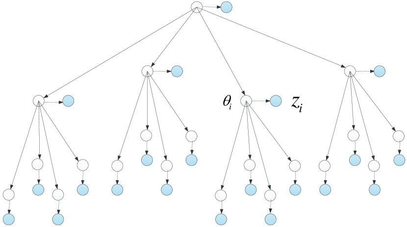
We now apply the max-product belief propagation algorithm [23, 24, 25] to each tree in our wavelet tree structure, with the goal to find the mode of $p_{\boldsymbol{\theta}_{\mathcal{T}}|\sigma^{2},\boldsymbol{z}}(\boldsymbol{\theta}_{\mathcal{T}}|\sigma^{2},\mbox{\boldmath$z$})$. We represent the hmt probabilistic model for $p_{\boldsymbol{\theta}_{\mathcal{T}}|\sigma^{2},\boldsymbol{z}}(\boldsymbol{\theta}_{\mathcal{T}}|\sigma^{2},\mbox{\boldmath$z$})$ via potential functions as [see (21b)]

$$p_{\boldsymbol{\theta}_{\mathcal{T}}|\sigma^{2},\boldsymbol{z}}(\boldsymbol{\theta}_{\mathcal{T}}|\sigma^{2},\mbox{\boldmath$z$})\propto\biggl{[}\prod_{i\in\mathcal{T}\backslash\mathcal{T}_{\textup{root}}}\psi_{i}(\boldsymbol{\theta}_{i})\psi_{i,\pi(i)}(q_{i},q_{\pi(i)})\biggr{]}\biggl{[}\prod_{i\in\mathcal{T}_{\textup{root}}}\psi_{i}(\boldsymbol{\theta}_{i})\biggr{]}$$ (23)

where

$$\psi_{i}(\boldsymbol{\theta}_{i}) = \mathcal{N}(z_{i}|s_{i},\sigma^{2})[\mathcal{N}(s_{i}|0,\gamma^{2}\sigma^{2})]^{q_{i}}[\mathcal{N}(s_{i}|0,\epsilon^{2}\sigma^{2})]^{1-q_{i}}$$ (24a)

for $$i\in\mathcal{T}\backslash\mathcal{T}_{\textup{root}}$$,

$$\psi_{i}(\boldsymbol{\theta}_{i}) = \mathcal{N}(z_{i}|s_{i},\sigma^{2})[P_{\textup{root}}\mathcal{N}(s_{i}|0,\gamma^{2}\sigma^{2})]^{q_{i}}[(1-P_{\textup{root}})\mathcal{N}(s_{i}|0,\epsilon^{2}\sigma^{2})]^{1-q_{i}}$$ (24b)

for $$i\in\mathcal{T}_{\textup{root}}$$, and

$$\psi_{i,\pi(i)}(q_{i},q_{\pi(i)}) = [{P_{\textup{H}}}^{q_{i}}(1-P_{\textup{H}})^{1-q_{i}}]^{q_{\pi(i)}}[{P_{\textup{L}}}^{q_{i}}(1-P_{\textup{L}})^{1-q_{i}}]^{1-q_{\pi(i)}}$$ (24c)

for $$i\in\mathcal{T}\backslash\mathcal{T}_{\textup{root}}$$.

Our algorithm for maximizing (23) consists of computing and passing upward and downward messages and calculating and maximizing beliefs.

III-A1 Computing and Passing Upward Messages

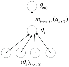
We propagate the upward messages from the lowest decomposition level (i.e., the leaves) towards the root of the tree. Fig. 3 depicts the computation of the upward message from variable node $\boldsymbol{\theta}_{i}$ to its parent node $\boldsymbol{\theta}_{\pi(i)}$ wherein we also define a child of $\boldsymbol{\theta}_{i}$ as a variable node $\boldsymbol{\theta}_{k}$ with index $k\in\mathop{\rm ch}\nolimits(i)$, where $\mathop{\rm ch}\nolimits(i)$ is the index set of the children of $i$: for $i=\upsilon(i_{1},i_{2})$, $\mathop{\rm ch}\nolimits(i)=\{\upsilon\big{(}(2i_{1}-1,2i_{2}-1),(2i_{1}-1,2i_{2}),(2i_{1},2i_{2}-1),(2i_{1},2i_{2})\big{)}\}$. Here, we use a circle and an edge with an arrow to denote a variable node and a message, respectively. The upward messages have the following general form [24]:

$$m_{i\rightarrow\pi(i)}(q_{\pi(i)})=\alpha\max_{\boldsymbol{\theta}_{i}}\biggl{\{}\psi_{i}(\boldsymbol{\theta}_{i})\psi_{i,\pi(i)}(q_{i},q_{\pi(i)})\prod_{k\in\mathop{\rm ch}\nolimits(i)}m_{k\rightarrow i}(q_{i})\biggr{\}}$$ (25)

where $\alpha>0$ denotes a normalizing constant used for computational stability [24]. For nodes with no children (corresponding to level $L$, i.e., $i\in\mathcal{T}_{{\scriptstyle{\rm leaf}}}$), we set the multiplicative term $\prod_{k\in\mathop{\rm ch}\nolimits(i)}m_{k\rightarrow i}(\boldsymbol{\theta}_{i})$ in (25) to one.

In Appendix B-I, we show that the only two candidates for $\boldsymbol{\theta}_{i}$ in the maximization of (25) are $[0,\widehat{s}_{i}(0)]^{T}$ and $[1,\widehat{s}_{i}(1)]^{T}$, see also (19).

Substituting these candidates into (25) and normalizing the messages yields (see Appendix B-I)

$$m_{i\rightarrow\pi(i)}(q_{\pi(i)})=[\mu^{\textup{u}}_{i}(0)]^{1-q_{\pi(i)}}[\mu^{\textup{u}}_{i}(1)]^{q_{\pi(i)}}$$ (26a)

where $$[\mu_{i}^{\textup{u}}(0),\mu_{i}^{\textup{u}}(1)]^{T}=\mbox{\boldmath$\mu$}_{i}^{\textup{u}}$$,

$$\mbox{\boldmath$\mu$}_{i}^{\textup{u}} = \frac{[\max\{\mbox{\boldmath$\nu$}_{0,i}^{\textup{u}}\odot\mbox{\boldmath$\eta$}_{i}^{\textup{u}}\},\max\{\mbox{\boldmath$\nu$}_{1,i}^{\textup{u}}\odot\mbox{\boldmath$\eta$}_{i}^{\textup{u}}\}]^{T}}{\max\{\mbox{\boldmath$\nu$}_{0,i}^{\textup{u}}\odot\mbox{\boldmath$\eta$}_{i}^{\textup{u}}\}+\max\{\mbox{\boldmath$\nu$}_{1,i}^{\textup{u}}\odot\mbox{\boldmath$\eta$}_{i}^{\textup{u}}\}}$$ (26b)

$$= \frac{\begin{bmatrix}\exp\bigl{(}\ln(\max\{\mbox{\boldmath$\nu$}_{0,i}^{\textup{u}}\odot\mbox{\boldmath$\eta$}_{i}^{\textup{u}}\})-\ln(\max\{\mbox{\boldmath$\nu$}_{1,i}^{\textup{u}}\odot\mbox{\boldmath$\eta$}_{i}^{\textup{u}}\})\bigr{)},&1\end{bmatrix}^{T}}{1+\exp\bigl{(}\ln(\max\{\mbox{\boldmath$\nu$}_{0,i}^{\textup{u}}\odot\mbox{\boldmath$\eta$}_{i}^{\textup{u}}\})-\ln(\max\{\mbox{\boldmath$\nu$}_{1,i}^{\textup{u}}\odot\mbox{\boldmath$\eta$}_{i}^{\textup{u}}\})\bigr{)}}$$

$$\mbox{\boldmath$\nu$}_{0,i}^{\textup{u}} = [1-P_{\textup{L}},P_{\textup{L}}]^{T}\odot\mbox{\boldmath$\phi$}(z_{i})$$ (26c)

$$\mbox{\boldmath$\nu$}_{1,i}^{\textup{u}} = [1-P_{\textup{H}},P_{\textup{H}}]^{T}\odot\mbox{\boldmath$\phi$}(z_{i})$$ (26d)

$$\mbox{\boldmath$\eta$}_{i}^{\textup{u}} = \begin{cases}\bigodot_{k\in\mathop{\rm ch}\nolimits(i)}\mbox{\boldmath$\mu$}^{\textup{u}}_{k},&i\in\mathcal{T}\backslash\mathcal{T}_{{\scriptstyle{\rm leaf}}}\\ [1,1]^{T},&i\in\mathcal{T}_{{\scriptstyle{\rm leaf}}}\end{cases}$$ (26e)

$$\mbox{\boldmath$\phi$}(z) = \begin{bmatrix}\exp(-0.5\frac{z^{2}}{\sigma^{2}+\sigma^{2}\epsilon^{2}})/\epsilon,&\exp(-0.5\frac{z^{2}}{\sigma^{2}+\sigma^{2}\gamma^{2}})/\gamma\end{bmatrix}^{T}$$ (26f)

and $\epsilon=\sqrt{\epsilon^{2}}>0$ and $\gamma=\sqrt{\gamma^{2}}>0$. A numerically stable implementation of (26b) that we employ is illustrated in the second expression in (26b). Similarly, the elementwise products in (26c)–(26e) are implemented as exponentiated sums of logarithms of the product terms.

Figure 3: Computing and passing (a) upward and (b) downward messages.

III-A2 Computing and Passing Downward Messages

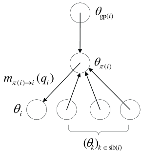
Upon obtaining all the upward messages, we now compute the downward messages and propagate them from the root towards the lowest level (i.e., the leaves). Fig. 3 depicts the computation of the downward message from the parent $\boldsymbol{\theta}_{\pi(i)}$ to the variable node $\boldsymbol{\theta}_{i}$, which involves upward messages to $\boldsymbol{\theta}_{\pi(i)}$ from its other children, i.e. the siblings of $\boldsymbol{\theta}_{i}$, marked as $\boldsymbol{\theta}_{k},k\in{\rm sib}(i)$. This downward message also requires the message sent to $\boldsymbol{\theta}_{\pi(i)}$ from its parent node, which is the grandparent of $\boldsymbol{\theta}_{i}$, denoted by $\boldsymbol{\theta}_{\operatorname{gp}(i)}$. The downward messages have the following general form [24]:

$$m_{\pi(i)\rightarrow i}(q_{i})=\alpha\max_{\boldsymbol{\theta}_{\pi(i)}}\Big{\{}\psi_{\pi(i)}(\boldsymbol{\theta}_{\pi(i)})\psi_{i,\pi(i)}(q_{i},q_{\pi(i)})m_{\operatorname{gp}(i)\rightarrow\pi(i)}(q_{\pi(i)})\prod_{k\in\operatorname{sib}(i)}m_{k\rightarrow\pi(i)}(q_{\pi(i)})\Big{\}}\hskip 18.06749pt$$ (27)

where $\alpha>0$ denotes a normalizing constant used for computational stability. For the variable nodes $i$ in the second decomposition level that have no grandparents (i.e., $\pi(i)\in\mathcal{T}_{\textup{root}}$), we set the multiplicative term $m_{\operatorname{gp}(i)\rightarrow\pi(i)}(q_{\pi(i)})$ in (27) to one.

In Appendix B-II, we show that the only two candidates for $\boldsymbol{\theta}_{\pi(i)}$ in the maximization of (27) are $[0,\widehat{s}_{\pi(i)}(0)]^{T}$ and $[1,\widehat{s}_{\pi(i)}(1)]^{T}$, see also (19). Substituting these candidates into (27) and normalizing the messages yields (see Appendix B-II)

$$m_{\pi(i)\rightarrow i}(q_{i})=[\mu_{i}^{\textup{d}}(0)]^{1-q_{i}}[\mu^{\textup{d}}_{i}(1)]^{q_{i}}$$ (28a)

for $$\pi(i)\in\mathcal{T}\backslash\mathcal{T}_{{\scriptstyle{\rm leaf}}} [\mu_{i}^{\textup{d}}(0),\mu_{i}^{\textup{d}}(1)]^{T}=\mbox{\boldmath$\mu$}_{i}^{\textup{d}}$$, where and

$$\mbox{\boldmath$\mu$}_{i}^{\textup{d}} = \frac{[\max\{\mbox{\boldmath$\nu$}_{0,i}^{\textup{d}}\odot\mbox{\boldmath$\eta$}_{i}^{\textup{d}}\},\max\{\mbox{\boldmath$\nu$}_{1,i}^{\textup{d}}\odot\mbox{\boldmath$\eta$}_{i}^{\textup{d}}\}]^{T}}{\max\{\mbox{\boldmath$\nu$}_{0,i}^{\textup{d}}\odot\mbox{\boldmath$\eta$}_{i}^{\textup{d}}\}+\max\{\mbox{\boldmath$\nu$}_{1,i}^{\textup{d}}\odot\mbox{\boldmath$\eta$}_{i}^{\textup{d}}\}}$$ (28b)

$$= \frac{\begin{bmatrix}\exp\bigl{(}\ln(\max\{\mbox{\boldmath$\nu$}_{0,i}^{\textup{d}}\odot\mbox{\boldmath$\eta$}_{i}^{\textup{d}}\})-\ln(\max\{\mbox{\boldmath$\nu$}_{1,i}^{\textup{d}}\odot\mbox{\boldmath$\eta$}_{i}^{\textup{d}}\})\bigr{)},&1\end{bmatrix}^{T}}{1+\exp\bigl{(}\ln(\max\{\mbox{\boldmath$\nu$}_{0,i}^{\textup{d}}\odot\mbox{\boldmath$\eta$}_{i}^{\textup{d}}\})-\ln(\max\{\mbox{\boldmath$\nu$}_{1,i}^{\textup{d}}\odot\mbox{\boldmath$\eta$}_{i}^{\textup{d}}\})\bigr{)}}$$

$$\mbox{\boldmath$\nu$}_{0,i}^{\textup{d}} = [1-P_{\textup{L}},1-P_{\textup{H}}]^{T}\odot\mbox{\boldmath$\phi$}(z_{\pi(i)})\odot\biggl{[}\bigodot_{k\in\operatorname{sib}(i)}\mbox{\boldmath$\mu$}^{\textup{u}}_{k}\biggr{]}$$ (28c)

$$\mbox{\boldmath$\nu$}_{1,i}^{\textup{d}} = [P_{\textup{L}},P_{\textup{H}}]^{T}\odot\mbox{\boldmath$\phi$}(z_{\pi(i)})\odot\biggl{[}\bigodot_{k\in\operatorname{sib}(i)}\mbox{\boldmath$\mu$}^{\textup{u}}_{k}\biggr{]}$$ (28d)

$$\mbox{\boldmath$\eta$}_{i}^{\textup{d}} = \begin{cases}[1-P_{\textup{root}},P_{\textup{root}}]^{T},&\pi(i)\in\mathcal{T}_{\textup{root}}\\ \mbox{\boldmath$\mu$}_{\pi(i)}^{\textup{d}},&\pi(i)\in(\mathcal{T}\backslash\mathcal{T}_{\textup{root}})\backslash\mathcal{T}_{{\scriptstyle{\rm leaf}}}\end{cases}.$$ (28e)

A numerically stable implementation of (28b) that we employ is illustrated in the second expression in (28b).

The above upward and downward messages have discrete representations, which is practically important and is a consequence of the fact that we use a Gaussian prior on the signal coefficients, see (5). Indeed, in contrast with the existing message passing algorithms for compressive sampling [9, 10, 11, 6], our max-product scheme employs exact messages.

III-A3 Maximizing Beliefs

Upon computing and passing all the upward and downward messages, we maximize the beliefs, which have the following general form [24]:

$$b(\boldsymbol{\theta}_{i})=\alpha\psi_{i}(\boldsymbol{\theta}_{i})m_{\pi(i)\rightarrow i}(q_{i})\prod_{k\in\mathop{\rm ch}\nolimits(i)}m_{k\rightarrow i}(q_{i})$$ (29)

for each $i\in\mathcal{T}$, where $\alpha>0$ is a normalizing constant. [In (29), we set $m_{\pi(i)\rightarrow i}(q_{i})=1$ if $i\in\mathcal{T}_{\textup{root}}$ and $\prod_{k\in\mathop{\rm ch}\nolimits(i)}m_{k\rightarrow i}(q_{i})=1$ if $i\in\mathcal{T}_{{\scriptstyle{\rm leaf}}}$.] We then use these beliefs to obtain the mode

$$\widehat{\boldsymbol{\theta}}_{\mathcal{T}}=\arg\max_{\boldsymbol{\theta}_{\mathcal{T}}}p_{\boldsymbol{\theta}_{\mathcal{T}}|\sigma^{2},\boldsymbol{z}}(\boldsymbol{\theta}_{\mathcal{T}}|\sigma^{2},\mbox{\boldmath$z$})$$ (30)

where the elements of $\widehat{\boldsymbol{\theta}}_{\mathcal{T}}$ are [see (19)]

$$\widehat{\boldsymbol{\theta}}_{i}=[\widehat{q}_{i},\widehat{s}_{i}(\widehat{q}_{i})]^{T}=\arg\max_{\boldsymbol{\theta}_{i}}b(\boldsymbol{\theta}_{i})=\begin{cases}[1,\widehat{s}_{i}(1)]^{T},&\beta_{i}(1)\geq\beta_{i}(0)\\ [0,\widehat{s}_{i}(0)]^{T},&\text{otherwise}\end{cases},\qquad i\in\mathcal{T}$$ (31a)

and

$$\mbox{\boldmath$\beta$}_{i}=[\beta_{i}(0),\beta_{i}(1)]^{T}=\begin{cases}\alpha_{1}[1-P_{\textup{root}},P_{\textup{root}}]^{T}\odot\mbox{\boldmath$\phi$}(z_{i})\odot\mbox{\boldmath$\eta$}_{i}^{\textup{u}},&i\in\mathcal{T}_{\textup{root}}\\ \alpha_{1}\mbox{\boldmath$\phi$}(z_{i})\odot\mbox{\boldmath$\mu$}_{i}^{\textup{d}}\odot\mbox{\boldmath$\eta$}_{i}^{\textup{u}},&i\in\mathcal{T}\backslash\mathcal{T}_{\textup{root}}\end{cases}.$$ (31b)

Here, $\alpha_{1}>0$ is a normalizing constant. The detailed derivation for the forms of $\widehat{\boldsymbol{\theta}}_{i}$ and $\mbox{\boldmath$\beta$}_{i}$ in (31) is provided in Appendix B-III.

IV Selecting $\sigma^{2}$ via Grid Search

We can integrate $\sigma^{2}$ out, yielding the marginal posterior of $\boldsymbol{\theta}$ in (13a), and derive an ‘outer’ em iteration for maximizing $p_{\boldsymbol{\theta}|\boldsymbol{y}}(\boldsymbol{\theta}|\boldsymbol{y})$:

1. fix $\sigma^{2}$ and apply the em iteration proposed in Section III to obtain an estimate $\boldsymbol{\theta}^{(+\infty)}(\sigma^{2})$ of $\boldsymbol{\theta}$;

2. fix $\boldsymbol{\theta}$ to the value obtained in (i) and estimate $\sigma^{2}$ as

   $$\widehat{\sigma}^{2}(\boldsymbol{\theta})=\frac{\|\boldsymbol{y}-H\boldsymbol{s}\|_{2}^{2}+\boldsymbol{s}^{T}D^{-1}(\mbox{\boldmath$q$})\boldsymbol{s}}{p+N}.$$ (32)

Even though it guarantees monotonic increase of the marginal posterior $p_{\boldsymbol{\theta}|\boldsymbol{y}}(\boldsymbol{\theta}|\boldsymbol{y})$, the ‘outer’ em iteration (1)–(2) does not work well in practice because it gets stuck in an undesirable local maximum of $p_{\boldsymbol{\theta}|\boldsymbol{y}}(\boldsymbol{\theta}|\boldsymbol{y})$. To find a better (generally local) maximum of $p_{\boldsymbol{\theta}|\boldsymbol{y}}(\boldsymbol{\theta}|\boldsymbol{y})$, we apply a grid search over $\sigma^{2}$ as follows.

Figure 4: Grid search for selecting $\sigma^{2}$.

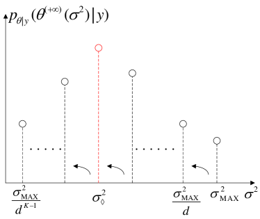
We apply the em algorithm in Section III using a range of values of the regularization parameter $\sigma^{2}$. We traverse the grid of $K$ values of $\sigma^{2}$ sequentially and use the signal estimate from the previous grid point to initialize the signal estimation at the current grid point (as depicted in Fig. 4): in particular, we move from a larger $\sigma^{2}$ (say $\sigma^{2}_{\text{old}}$) to the next smaller $\sigma^{2}_{\text{new}}(<\sigma^{2}_{\text{old}})$ and use $\boldsymbol{s}^{(+\infty)}(\sigma^{2}_{\text{old}})$ (obtained upon convergence of the em iteration in Section III for $\sigma^{2}=\sigma^{2}_{\text{old}}$) to initialize the em iteration at $\sigma^{2}_{\text{new}}$. The largest $\sigma^{2}$ on the grid and the initial signal estimate at this grid point are selected as

$$\sigma_{\textup{MAX}}^{2}=\frac{\|\boldsymbol{y}\|_{2}^{2}}{p+N},\quad\boldsymbol{\theta}^{(0)}(\sigma_{\textup{MAX}}^{2})=\mathbf{0}_{2p\times 1}.$$ (33a)

The consecutive grid points $$\sigma^{2}_{\text{new}} \sigma^{2}_{\text{old}}$$ and satisfy

$$\sigma^{2}_{\text{new}}=\frac{\sigma^{2}_{\text{old}}}{d}$$ (33b)

where $$d>1$$ is a constant determining the search resolution.

Finally, we select the $\sigma^{2}$ from the above grid of candidates that yields the largest marginal posterior distribution (13a):

$$\sigma_{\diamondsuit}^{2}=\arg\max_{\sigma^{2}\in\{\sigma_{\textup{MAX}}^{2},\sigma_{\textup{MAX}}^{2}/d,\ldots,\sigma_{\textup{MAX}}^{2}/d^{K-1}\}}p_{\boldsymbol{\theta}|\boldsymbol{y}}(\boldsymbol{\theta}^{(+\infty)}(\sigma^{2})|\boldsymbol{y})$$ (34)

and the final estimates of $\boldsymbol{\theta}$ and $\boldsymbol{s}$ as $\boldsymbol{\theta}^{(+\infty)}(\sigma_{\diamondsuit}^{2})$ and $\boldsymbol{s}^{(+\infty)}(\sigma_{\diamondsuit}^{2})$, respectively, see Fig. 4.

V Numerical Examples

We compare the reconstruction performances of the following methods:

• our proposed max-product em (mp-em) algorithm in Section III with the variance parameter $\sigma^{2}$ selected via grid search using the marginal-posterior based criterion in Section IV, search resolution $d=2$, and zero initial signal estimate:

  $$\boldsymbol{s}^{(0)}={\bf 0}_{p\times 1}$$ (35)

  with Matlab implementations available at http://home.eng.iastate.edu/~ald/MPEM.html;

• our mp-em algorithm in Section III with $\sigma^{2}$ tuned manually for good performance (labeled mp-em${}_{\textsc{opt}}$) with $d=2$ and zero $\boldsymbol{s}^{(0)}$ in (35), used as a benchmark;

• the Gaussian-mixture version of the turbo-amp approach [6] with a Matlab implementation in [26] and the tuning hyperparameters chosen as the default values in this implementation;

• the fixed-point continuation active set (fpc${}_{\textsc{as}}$) algorithm [27] that aims at minimizing the Lagrangian cost function

  $$0.5\|\boldsymbol{y}-H\boldsymbol{s}\|_{2}^{2}+\tau\|\boldsymbol{s}\|_{1}$$ (36a)

  with the regularization parameter $$\tau$$ computed as

  $$\tau=10^{a}\|H^{T}\boldsymbol{y}\|_{\infty}$$ (36b)

  where $a$ is a tuning parameter chosen manually to achieve good reconstruction performance;

• the Barzilai-Borwein version of the gradient-projection for sparse reconstruction (gpsr) method with debiasing in [28, Sec. III.B] with the convergence threshold $\texttt{tolP}=10^{-5}$ and tuning parameter $a$ in (36b) chosen manually to achieve good reconstruction performance;

• the normalized iterative hard thresholding (niht) scheme [29] initialized by the zero $\boldsymbol{s}^{(0)}$ in (35);

• the model-based iterative hard thresholding (mb-iht) algorithm [7] using a greedy tree approximation [30], initialized by the zero $\boldsymbol{s}^{(0)}$ in (35);

• the vb tree-structured compressive sensing [5] with a Matlab implementation in [31] and the tuning hyperparameters chosen as the default values in this implementation.

For the mp-em, niht, and mb-iht iterations, we use the following convergence criterion:

$$\frac{\|\boldsymbol{s}^{(j+1)}-\boldsymbol{s}^{(j)}\|_{2}^{2}}{p}<\delta$$ (37)

where $\delta>0$ is the convergence threshold selected in the following examples so that the performances of the above methods do not change significantly by further decreasing $\delta$.

For mp-em, we set the tuning constants in all following examples as

$$\gamma^{2}=1000,\quad\epsilon^{2}=0.1,\quad P_{\textup{root}}=P_{\textup{H}}=0.2,\quad P_{\textup{L}}=10^{-5}$$ (38)

which leads to $\frac{\operatorname{E}\left[\sum_{i=1}^{p}q_{i}\right]}{p}=0.0108$.

The sensing matrix $H$ has the following structure:

$$H=\frac{1}{\rho_{\Phi}}\Phi\Psi$$ (39)

where $\Phi$ is the $N\times p$ sampling matrix and $\Psi$ is the $p\times p$ orthogonal transform matrix (satisfying $\Psi\Psi^{T}=I_{p}$). Note that $H$ in (39) satisfies the spectral norm condition (3). We set the tree depth

$$L=4.$$ (40)

V-A Small-scale Structured Sparse Signal Reconstruction

We generated the binary state variables $q$ of length $p=1024$ using the Markov tree model in Section II. Conditional on $q_{i}$, $s_{i}$ are generated according to (5b). Here, the matrix-to-vector conversion operator $\upsilon(\cdot)$ corresponds to simple columnwise conversion, except for vb whose implementation [31] requires the use of Matlab’s wavedec2 function for this purpose. The sampling matrices $\Phi$ in (39) have been simulated using

1. a white Gaussian matrix whose entries are i.i.d. standard Gaussian random variables,

2. a row-correlated Gaussian matrix with i.i.d. zero-mean Gaussian columns (indexed by $k=1,2,\ldots,p$) having covariance matrix whose $(i,j)$th element is

   $$\operatorname{cov}(\Phi_{i,k},\Phi_{j,k})=r^{|i-j|},\qquad i,j=1,2,\ldots,N$$ (41a)

   useful, e.g., in modeling time-series data [32, Sec. 5], and

3. a column-correlated Gaussian matrix with i.i.d. zero-mean Gaussian rows (indexed by $k=1,2,\ldots,N$) having covariance matrices whose $(i,j)$th element is

   $$\operatorname{cov}(\Phi_{k,i},\Phi_{k,j})=c^{|i-j|},\qquad i,j=1,2,\ldots,p.$$ (41b)

The general column correlation model (3) for the design (sensing) matrices is analyzed in [32, 33, 34], see also [35, 36, 37], which employ this correlation structure. Correlations among columns of the design matrices occur e.g., in genomic applications [38, Sec. 18.4] and spatially correlated designs are relevant to functional magnetic resonance imaging (fmri) [39].

The transform matrix $\Psi$ in (39) is chosen to be identity:

$$\Psi=I_{p}$$ (42)

hence, in this example, the sampling and sensing matrices $\Phi$ and $H$ are the same up to a proportionality constant.

We simulate the observation vectors $\boldsymbol{y}$ using the measurement and prior models in (2), (5), and (6) and following model parameters:

$$\epsilon_{\star}^{2}=1,\quad\sigma_{\star}^{2}=10^{-6},\quad(P_{\textup{root}})_{\star}=(P_{\textup{H}})_{\star}=0.5,\quad(P_{\textup{L}})_{\star}=10^{-4},\quad\gamma_{\star}^{2}\in\{10^{3},10^{4},10^{5}\}$$ (43)

where the subscripts $\star$ emphasize that these selections are the true model parameters employed to simulate the measurements and are generally different from the tuning constants (38) employed by the mp-em method. Here, our goal is to show the performance of the mp-em method in the case where there is a mismatch between the tuning parameters and corresponding true model parameters. The choices $(P_{\textup{H}})_{\star},(P_{\textup{root}})_{\star}$, and $(P_{\textup{L}})_{\star}$ in (43) correspond to the normalized expected number of large-magnitude signal coefficients

$$\frac{\operatorname{E}\bigl{[}\sum_{i=1}^{p}q_{i}\bigr{]}}{p}=0.0919$$ (44)

computed using (7a). We vary the values of $\gamma_{\star}^{2}$ to test the performances of various methods at different signal-to-noise ratios (snrs).

Our performance metric is the average normalized mean-square error (nmse) of an estimate $\widetilde{\boldsymbol{s}}$ of the signal coefficient vector (used also in e.g., [40]):

$$\operatorname{NMSE}\{\widetilde{\boldsymbol{s}}\}=\operatorname{E}_{\Phi,\boldsymbol{s},\boldsymbol{y}}\biggl{[}\frac{\|\widetilde{\boldsymbol{s}}-\boldsymbol{s}\|^{2}_{2}}{\|\boldsymbol{s}\|_{2}^{2}}\biggr{]}$$ (45)

computed using $500$ Monte Carlo trials, where averaging is performed over the random Gaussian sampling matrices $\Phi$, signal $\boldsymbol{s}$, and measurements $\boldsymbol{y}$.

We select the convergence threshold in (37) to

$$\delta=10^{-10}.$$ (46)

For mp-em and mp-em${}_{\textsc{opt}}$, we set the grid length $K=16$. The tuning parameters for mp-em are given in (38).

The niht and mb-iht methods require knowledge of the signal sparsity level (i.e., an upper bound on the number of nonzero coefficients); in this example, we set the signal sparsity level for these methods to the exact number of large-magnitude signal coefficients $\sum_{i=1}^{p}q_{i}$. For gpsr and fpc${}_{\textsc{as}}$, we vary $a$ in (36b) within the set $\{-1,-2,-3,-4,-5,-6,-7,-8,-9\}$ and, for each $N/p$ and each of the two methods, we use the optimal $a$ that achieves the smallest nmse.

The turbo-amp implementation in [26] requires a function input xRange that corresponds to the range of the input signal $\Psi\boldsymbol{s}$. In this example, we set the value of this tuning constant to six standard deviations of the signal coefficients in $\boldsymbol{s}$:

$$\texttt{xRange}=6\sigma_{\star}\sqrt{\frac{\operatorname{E}\bigl{[}\sum_{i=1}^{p}q_{i}\bigr{]}}{p}\gamma_{\star}^{2}+\Bigl{(}1-\frac{\operatorname{E}\bigl{[}\sum_{i=1}^{p}q_{i}\bigr{]}}{p}\Bigr{)}\epsilon_{\star}^{2}}$$ (47)

where $\sigma_{\star}=\sqrt{\sigma_{\star}^{2}}$; turbo-amp with this selection performs well compared with other choices of xRange that we tested. Selecting too small or too large xRange would lead to deteriorated performance of turbo-amp. Turbo-amp is particularly sensitive to underestimation of this quantity and less sensitive to selecting larger values than optimal.

V-A1 White and Row-correlated Sensing Matrices

Fig. 5 shows the nmses of different methods as functions of the subsampling factor $N/p$ for the three choices of $\gamma_{\star}^{2}$ in (43), corresponding to relatively low, medium, and high snrs, and white and row-correlated sensing matrices with correlation parameter $r=0.2$ in (41a). Here, a larger value of the high-signal relative variance $\gamma_{\star}^{2}$ implies a relatively higher snr. Indeed, for each method, the signal with higher snr can be reconstructed with a smaller nmse than the signal with lower snr: Compare Figs. 5, 5, and 5 as well as Figs. 5, 5, and 5.

Figure 5: nmses as functions of the subsampling factor $N/p$ for (a)-(b) low snr with $\gamma_{\star}^{2}=10^{3}$, (c)-(d) medium snr with $\gamma_{\star}^{2}=10^{4}$, and (e)-(f) high snr with $\gamma_{\star}^{2}=10^{5}$ using [left: (a), (c), (e)] white and [right: (b), (d), (f)] row-correlated sensing matrices with correlation parameter $r=0.2$, respectively.

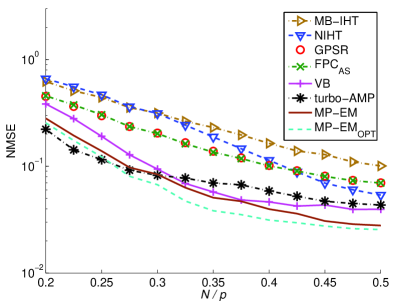
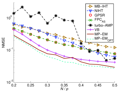
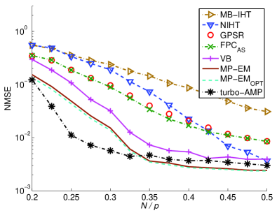
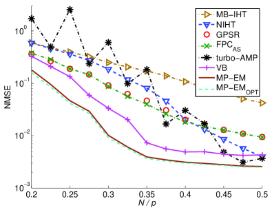
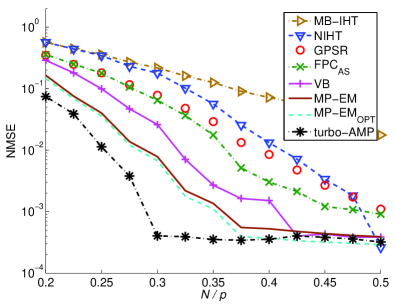
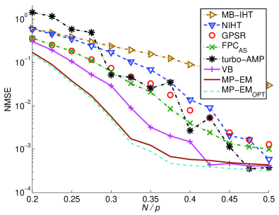
For white Gaussian sampling matrices, the methods that employ the probabilistic tree structure of the signal coefficients (turbo-amp, mp-em, mp-em${}_{\textsc{opt}}$, and vb) clearly outperform all other approaches, see Figs. 5, 5, and 5. For row-correlated Gaussian sampling matrices, mp-em and mp-em${}_{\textsc{opt}}$ achieve the best overall performances, followed by the vb method; turbo-amp is sensitive to introducing correlation among elements of the sampling matrix $\Phi$ and performs poorly for smaller $N/p$, see Figs. 5, 5, and 5.

For white Gaussian sampling matrices, we observe the following:

• at low snr, mp-em and mp-em${}_{\textsc{opt}}$ outperform other approaches when $N/p>0.275$, see Fig. 5;

• at medium and high snrs, turbo-amp achieves the best overall performance, followed by mp-em${}_{\textsc{opt}}$ and mp-em, see Figs. 5 and 5.

The niht method performs relatively poorly for smaller $N/p$, but improves as $N/p$ increases. For sufficiently high $N/p$, niht achieves smaller nmses than other methods that do not exploit the probabilistic tree structure.

In Fig. 5, the nmses of mp-em are close to those of mp-em${}_{\textsc{opt}}$, which implies that the marginal-posterior based criterion in Section IV selects the noise variance parameter well in this example.

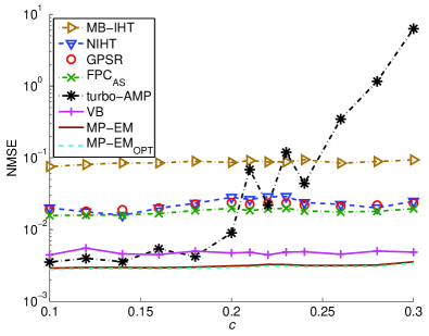
The performance of turbo-amp deteriorates with introduction of correlation among elements of the sampling matrix $\Phi$: The nmses of turbo-amp for some subsampling factors are more than an order of magnitude larger for row-correlated sampling matrices than for white sampling matrices. In contrast, the nmses for all the other methods increase only slightly when we introduce sampling matrix correlation (41a), compare the left and right-hand sides of Fig. 5. Increasing this correlation by increasing $r$ to $0.3$ in (41a) results in further performance deterioration of turbo-amp (i.e., turbo-amp has very high nmses for all $N/p$ in this case), whereas the competing methods continue to perform well.

Figure 6: Column-correlated sensing matrices: nmses as functions of (a) the subsampling factor $N/p$ for correlation parameter $c=0.2$ and (b) $c$ for $N/p=0.4$ under the medium snr scenario with $\gamma_{\star}^{2}=10^{4}$.

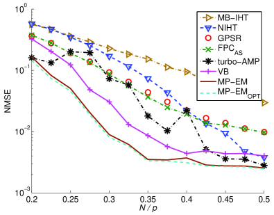
The vb method performs well under both white and row-correlated sensing matrix scenarios and turbo-amp has a superior reconstruction performance under the white sensing matrix scenario. These good performances are likely facilitated by the fact that vb and turbo-amp learn the Markov tree parameters from the measurements.

V-A2 Column-correlated Sensing Matrices

Fig. 6 shows the nmses of different methods as functions of the subsampling factor $N/p$ for column-correlated sampling matrices having the correlation constant $c=0.2$ in (41b) under the medium snr scenario. Here, mp-em and mp-em${}_{\textsc{opt}}$ have the smallest nmses over nearly the entire range of $N/p$ considered. Fig. 6 shows the nmses as functions of $c$ for $N/p$ fixed at $0.4$. Here, only turbo-amp is very sensitive to the presence of correlations among the elements of the sampling matrix, whereas all other methods vary only slightly as functions of $c$.

We also observe numerical instability of turbo-amp when correlated Gaussian sampling matrices are employed, which is exhibited by the oscillatory behavior of its nmses in the right side of Fig. 5 and in Fig. 6 [demanding more averaging than the $500$ Monte Carlo trials that we employ to estimate (45)].

We simulated sampling matrices $\Phi$ that have variable column norms or row norms, which led to deteriorating performances of turbo-amp in both cases, whereas the competing methods perform well. The fact that turbo-amp has been derived assuming Gaussian sensing matrices with i.i.d. elements explains its poor performance for sensing matrices that deviate sufficiently from this assumption.

The mb-iht method, which employs a greedy tree approximation and deterministic tree structure, achieves quite a poor nmse performance in Figs. 5 and 6. A relatively poor performance of mb-cosamp (which employs the same deterministic tree structure) has also been reported in [6, Sec. IV.B].

V-B Image Reconstruction

We reconstruct $128\times 128$ and $256\times 256$ test images from noiseless compressive samples ($\sigma_{\star}^{2}=0$). Here, the matrix-to-vector conversion operator $\upsilon(\cdot)$ is based on the columnwise conversion for $128\times 128$ images, and Matlab wavelet decomposition function wavedec2 with Haar wavelet for $256\times 256$ images, which has also been used in [4] and [6]. Before taking the wavelet transform, we subtract the mean of original image to ensure that $\Psi\boldsymbol{s}$ has zero mean.

For turbo-amp, we set the function input xRange to $255$, which is the difference between the minimum and maximum possible image values in this example. Observe that the turbo-amp implementation in [26] needs additional prior information about the signal range, which is not required by other methods.

V-B1 Medium scale with row-correlated Gaussian sampling matrices

We reconstruct the $128\times 128$ ‘Cameraman’ image (cropped from the original $256\times 256$ image in Fig. 9(b), as was also done in [31, 26] and corresponding papers [5, 6]) from compressive samples generated using row-correlated Gaussian sampling matrices with covariances between the elements described by (41a). Our performance metric is the nmse in (45) computed using $10$ Monte Carlo trials, where the averaging is performed only over the random Gaussian sampling matrices $\Phi$.

In this example, the convergence threshold in (37) is set to

$$\delta=0.01.$$ (48)

For mp-em and mp-em${}_{\textsc{opt}}$, we set the grid length $K=16$. The tuning parameters for mp-em are given in (38).

We set the sparsity level $r$ for niht as $2000N/p$ and $2500N/p$ for mb-iht, tuned for good nmse performance.

Figure 7: (a) nmses and (b) cpu times as functions of the correlation parameter $r$ for the $128\times 128$ ‘Cameraman’ image when $N/p=0.3$.

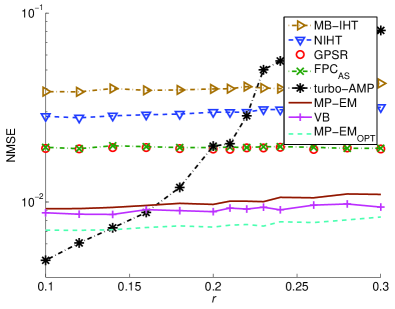
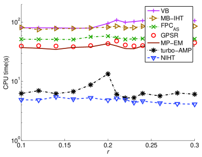
Fig. 7 shows the nmses and cpu times of different methods reconstructing the $128\times 128$ ‘Cameraman’ image as functions of the correlation parameter $r$ in (41a) with $N/p=0.3$. Since mp-em and mp-em${}_{\textsc{opt}}$ have the same runtime, we report only that of mp-em in Fig. 7. Turbo-amp has the smallest nmse when $N/p\leq 0.12$. However, its nmse increases sharply as $r$ becomes larger: turbo-amp has the largest nmse when $N/p>0.22$. In contrast, the nmses for all the other methods keep nearly constants as we increase $r$. The mp-em, mp-em${}_{\textsc{opt}}$, and vb methods have smaller nmses than gpsr, fpc${}_{\textsc{as}}$, niht, and mb-iht for all the correlation coefficients $r$ considered. The vb approach performs slightly better than mp-em, but is slower than mp-em and mp-em${}_{\textsc{opt}}$. In terms of cpu time, niht is the fastest among all the methods compared and turbo-amp requires $0.3\text{\,}\mathrm{s}8.6\text{\,}\mathrm{s}$ more than niht, both of which are faster than the remaining methods. The vb scheme consumes the largest amount of cpu time among all the methods for all the correlation coefficient $r$ considered; mp-em and mp-em${}_{\textsc{opt}}$ are faster than gpsr, fpc${}_{\textsc{as}}$, mb-iht, and vb.

As before, the good performance of vb is likely facilitated by the fact that it learns the Markov tree parameters from the measurements.

Fig. 8 shows the reconstructed $128\times 128$ ‘Cameraman’ image by different methods for $N/p=0.3$ and $r=0.2$ using one realization of the sampling matrix $\Phi$. In Fig. 8, we also report the peak signal-to-noise ratios (psnrs) of these methods, where the psnr of an estimated signal $\widetilde{\boldsymbol{s}}$ is defined as [41, eq. (3.7)]:

$$\mbox{PSNR}~{}\text{(dB)}=10\log_{10}\biggl{\{}\frac{[(\Psi\boldsymbol{s})_{\textup{MAX}}-(\Psi\boldsymbol{s})_{\textup{MIN}}]^{2}}{\|\widetilde{\boldsymbol{s}}-\boldsymbol{s}\|^{2}_{2}/p}\biggr{\}}.$$ (49)

(a) mp-em${}_{\textsc{opt}}$ (psnr $26.3\text{\,}\mathrm{dB}$)

(b) vb (psnr $25.8\text{\,}\mathrm{dB}$)

(c) mp-em (psnr $24.9\text{\,}\mathrm{dB}$)

(d) turbo-amp (psnr $23.8\text{\,}\mathrm{dB}$)

(e) fpc${}_{\textsc{as}}$ (psnr $22.0\text{\,}\mathrm{dB}$)

(f) gpsr (psnr $22.0\text{\,}\mathrm{dB}$)

(g) niht (psnr $20.2\text{\,}\mathrm{dB}$)

(h) mb-iht (psnr $18.7\text{\,}\mathrm{dB}$)

Figure 8: The $128\times 128$ ‘Cameraman’ image reconstructed by various methods for $r=0.2$ and $N/p=0.3$.

V-B2 Large scale with structurally random sampling matrices

We now reconstruct several $256\times 256$ test images shown in Fig. 9 from compressive samples. The sampling matrix $\Phi$ is generated using structurally random compressive samples [42] and the transform matrix $\Psi$ in (39) is the $p\times p$ orthogonal inverse Haar wavelet transform matrix, which implies that the sensing matrix $H$ has orthonormal rows: $HH^{T}=I_{N}$ and, consequently, $\rho_{\Phi}=\rho_{H}=1$. Our performance metric in this example is the psnr, see (49).

In this example, the convergence threshold in (37) is set to

$$\delta=0.1.$$ (50)

For mp-em and mp-em${}_{\textsc{opt}}$, we set the grid length $K=12$. The tuning parameters for mp-em are the same as before and given in (38).

We set the signal sparsity levels for niht and mb-iht to $10000N/p$ and $15000N/p$, respectively, tuned for good psnr performance. For fpc${}_{\textsc{as}}$ and gpsr, we set the regularization parameter $a=-3$ [see (36b)], which yields generally the best psnr performance for these two methods.

We do not include the vb method in this example because its implementation [31] cannot be applied to reconstruct the large-scale images in Fig. 9.

(a) Lena

(b) Cameraman

(c) House

(d) Boat

(e) Einstein

(f) Peppers

(g) Couple

Figure 9: The $256\times 256$ test images.

Figure 10: (a) psnrs and (b) cpu times as functions of the subsampling factor $N/p$ for the $256\times 256$ ‘Cameraman’ image.

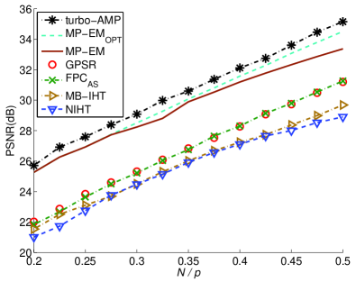
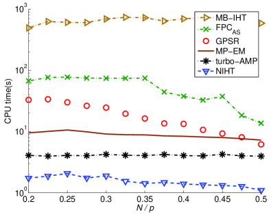
Fig. 10 shows the psnrs and cpu times of different methods reconstructing the $256\times 256$ ‘Cameraman’ image, as functions of the subsampling factor $N/p$. Turbo-amp has the highest psnrs for all $N/p$. The performances of mp-em and mp-em${}_{\textsc{opt}}$ are close to that of turbo-amp: the psnrs of mp-em${}_{\textsc{opt}}$ are $0.4\text{\,}\mathrm{dB}0.7\text{\,}\mathrm{dB}$ less than those of turbo-amp. Moreover, the psnr improvement for mp-em against its other closest competitors varies between $2.1\text{\,}\mathrm{dB}3.2\text{\,}\mathrm{dB}$. In terms of cpu time, niht is the fastest among all the methods compared; turbo-amp is the second fastest and takes around $4\text{\,}\mathrm{s}$ for each $N/p$. The mp-em method requires $3.3\text{\,}\mathrm{s}6.5\text{\,}\mathrm{s}$ more than turbo-amp, but is clearly faster than gpsr, fpc${}_{\textsc{as}}$, and mb-iht for nearly all measurement points. As before, mp-em and mp-em${}_{\textsc{opt}}$ have the same runtime and we report only that of mp-em in Fig. 10.

Table I shows the psnrs of the compared methods for different images and $N/p$ equal to $0.35$. The mp-em, mp-em${}_{\textsc{opt}}$, and turbo-amp methods clearly outperform the other methods for every image. In Table I, turbo-amp is better than mp-em${}_{\textsc{opt}}$ and mp-em for all the images: The improvement in terms of psnr varies between $0.3\text{\,}\mathrm{dB}$ and $1.4\text{\,}\mathrm{dB}$.

TABLE I: psnrs for $N/p=0.35$.

	niht	mb-iht	fpc${}_{\textsc{as}}$	gpsr	turbo-amp	mp-em	mp-em${}_{\textsc{opt}}$
Lena	24.3	24.8	25.3	25.5	29.2	27.8	27.9
Cameraman	26.0	26.0	26.8	26.8	30.6	29.9	30.1
House	29.8	29.7	30.5	30.5	33.4	32.6	33.1
Boat	22.5	22.9	23.7	24.0	27.1	26.1	26.1
Einstein	26.9	27.4	27.4	27.7	30.4	30.0	30.0
Peppers	25.8	26.2	26.1	26.2	30.2	29.2	29.3
Couple	28.8	29.1	30.3	30.2	33.6	32.6	32.7

In Fig. 10 and Table I, mb-iht achieves a fair performance and consumes the the largest amount of cpu time. Turbo-amp performs well for all $N/p$ and images and outperforms all competitors, which is likely because

• it uses a more general prior on the binary state variables (than our mp-em method), which allows the tree probability parameters $P_{\textup{H}}$, $P_{\textup{L}}$, $\gamma^{2}$, and $\epsilon^{2}$ to vary between the signal decomposition levels, and

• learns the tree probability parameters parameters from the measurements.

In contrast, our mp-em method employs the crude choices of the tree and other tuning parameters in (38).

(a) True Image

(b) turbo-amp ($\lx@glossaries@gls@link{acronym}{PSNR}{\leavevmode\textsc{psnr}}=30.59$ dB)

(c) mp-em${}_{\textsc{opt}}$ ($\lx@glossaries@gls@link{acronym}{PSNR}{\leavevmode\textsc{psnr}}=30.08$ dB)

(d) mp-em ($\lx@glossaries@gls@link{acronym}{PSNR}{\leavevmode\textsc{psnr}}=29.89$ dB)

(e) gpsr ($\lx@glossaries@gls@link{acronym}{PSNR}{\leavevmode\textsc{psnr}}=26.83$ dB)

(f) fpc${}_{\textsc{as}}$ ($\lx@glossaries@gls@link{acronym}{PSNR}{\leavevmode\textsc{psnr}}=26.75$ dB)

(g) mb-iht ($\lx@glossaries@gls@link{acronym}{PSNR}{\leavevmode\textsc{psnr}}=26.01$ dB)

(h) niht ($\lx@glossaries@gls@link{acronym}{PSNR}{\leavevmode\textsc{psnr}}=25.91$ dB)

Figure 11: The ‘Cameraman’ image reconstructed by various methods for $N/p=0.35$.

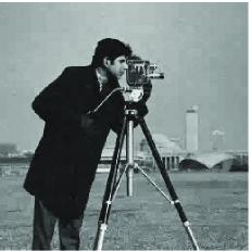
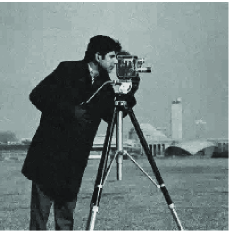
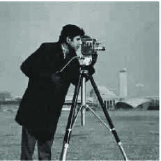
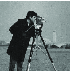
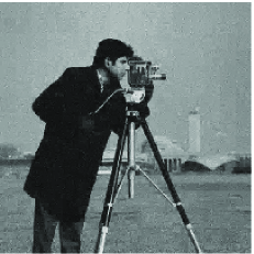
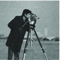
Fig. 11 shows the reconstructed $256\times 256$ ‘Cameraman’ image by different methods for $N/p=0.35$: In this case, the turbo-amp algorithm achieves the best reconstructed image quality compared with other methods, followed closely by mp-em and mp-em${}_{\textsc{opt}}$; the reconstructions of all other methods are clearly inferior to these schemes.

VI Concluding Remarks

We presented a Bayesian em algorithm for reconstructing approximately sparse signal from compressive samples using a Markov tree prior for the signal coefficients. We employed the max-product belief propagation algorithm to implement the m step of the proposed em iteration. Compared with the existing message passing algorithms in the compressive sampling area, our method does not approximate the message form. The simulation results show that our algorithm often outperforms existing algorithms for simulated signals and standard test images with different sampling operators and can successfully reconstruct signals collected by sampling matrices with correlated elements and variable norms of rows and columns.

Our future work will include the convergence analysis of the mp-em algorithm, incorporating other measurement models, using a more general prior distribution for the binary state variables, and designing schemes for learning the probabilistic Markov tree parameters from the measurements.

Appendix A Derivation of the MP-EM Iteration and Proofs of Its Monotonicity and Theorem 1

We first determine the complete-data posterior distribution and the distribution of the missing data $\boldsymbol{z}$ given the observed data $\boldsymbol{y}$ and parameters $\boldsymbol{\theta}$ and $\sigma^{2}$. We then use these distributions to derive the em iteration in Section III following the standard approach outlined in, e.g., [16, Sec. 12.3]. Finally, we prove the monotonicity of the mp-em iteration in (17) and Theorem 1.

Consider the hierarchical two-stage model in (14). The complete-data posterior distribution for known $\sigma^{2}$ is

$$p_{\boldsymbol{\theta},\boldsymbol{z}|\sigma^{2},\boldsymbol{y}}(\boldsymbol{\theta},\mbox{\boldmath$z$}|\sigma^{2},\boldsymbol{y}) \propto p_{\boldsymbol{y}|\boldsymbol{z},\sigma^{2}}(\boldsymbol{y}|\boldsymbol{z},\sigma^{2})p_{\boldsymbol{z}|\boldsymbol{s}}(\boldsymbol{z}|\boldsymbol{s})p_{\boldsymbol{s}|\boldsymbol{q},\sigma^{2}}(\boldsymbol{s}|\boldsymbol{q},\sigma^{2})p_{\boldsymbol{q}}(\boldsymbol{q})$$ (A1a)

$$\propto \frac{\exp\{-0.5(\boldsymbol{y}-H\mbox{\boldmath$z$})^{T}[C(\sigma^{2})]^{-1}(\boldsymbol{y}-H\mbox{\boldmath$z$})\}}{\sqrt{\det[C(\sigma^{2})]}}\Bigl{(}\frac{\epsilon^{2}}{\gamma^{2}}\Bigr{)}^{0.5\sum_{i=1}^{p}q_{i}}p_{\boldsymbol{q}}(\mbox{\boldmath$q$})$$

$$\cdot\exp[-0.5\|\mbox{\boldmath$z$}-\boldsymbol{s}\|_{2}^{2}/\sigma^{2}-0.5\boldsymbol{s}^{T}D^{-1}(\mbox{\boldmath$q$})\boldsymbol{s}/\sigma^{2}]$$

where

$$C(\sigma^{2})=\sigma^{2}(I_{N}-HH^{T}).$$ (A1b)

Consequently, the distribution of the missing data $$\boldsymbol{z} \boldsymbol{y} \boldsymbol{\theta} \sigma^{2}$$ given the observed data and parameters and is

$$p_{\boldsymbol{z}|\sigma^{2},\boldsymbol{y},\boldsymbol{\theta}}(\mbox{\boldmath$z$}|\sigma^{2},\boldsymbol{y},\boldsymbol{\theta})=p_{\boldsymbol{z}|\sigma^{2},\boldsymbol{y},\boldsymbol{s}}(\mbox{\boldmath$z$}|\sigma^{2},\boldsymbol{y},\boldsymbol{s})=\mathcal{N}\bigl{(}\mbox{\boldmath$z$}|\operatorname{E}_{\boldsymbol{z}|\sigma^{2},\boldsymbol{y},\boldsymbol{s}}(\mbox{\boldmath$z$}|\sigma^{2},\boldsymbol{y},\boldsymbol{s}),\operatorname{cov}_{\boldsymbol{z}|\sigma^{2},\boldsymbol{y},\boldsymbol{s}}(\mbox{\boldmath$z$}|\sigma^{2},\boldsymbol{y},\boldsymbol{s})\bigr{)}$$

where

$$\operatorname{E}_{\boldsymbol{z}|\sigma^{2},\boldsymbol{y},\boldsymbol{s}}(\mbox{\boldmath$z$}|\sigma^{2},\boldsymbol{y},\boldsymbol{s}) = \{H^{T}[C(\sigma^{2})]^{-1}H+I_{p}/\sigma^{2}\}^{-1}\{H^{T}[C(\sigma^{2})]^{-1}\boldsymbol{y}+\boldsymbol{s}/\sigma^{2}\}$$ (A1d)

$$\operatorname{cov}_{\boldsymbol{z}|\sigma^{2},\boldsymbol{y},\boldsymbol{s}}(\mbox{\boldmath$z$}|\sigma^{2},\boldsymbol{y},\boldsymbol{s}) = \{H^{T}[C(\sigma^{2})]^{-1}H+I_{p}/\sigma^{2}\}^{-1}.$$ (A1e)

By using the matrix inversion lemma [43, eq. (2.22), p. 424]:

$$(R+STU)^{-1} = R^{-1}-R^{-1}S(T^{-1}+UR^{-1}S)^{-1}UR^{-1}$$ (A2a)

and the following identity [43, p. 425]:

$$(R+STU)^{-1}ST = R^{-1}S(T^{-1}+UR^{-1}S)^{-1}$$ (A2b)

we simplify the conditional mean of the missing data in (A1d) to the familiar backprojection form:

$$\operatorname{E}_{\boldsymbol{z}|\sigma^{2},\boldsymbol{y},\boldsymbol{s}}[\mbox{\boldmath$z$}|\sigma^{2},\boldsymbol{y},\boldsymbol{s}]=\boldsymbol{s}+H^{T}(\boldsymbol{y}-H\boldsymbol{s}).$$ (A3)

We now derive the em iteration in Section III by noting that the objective function $\ln p_{\boldsymbol{\theta}|\sigma^{2},\boldsymbol{y}}(\boldsymbol{\theta}|\sigma^{2},\boldsymbol{y})$ that we aim to maximize satisfies the following property [see e.g., [16, eq. (12.4)]]:

$$\ln p_{\boldsymbol{\theta}|\sigma^{2},\boldsymbol{y}}(\boldsymbol{\theta}|\sigma^{2},\boldsymbol{y})={\cal Q}(\boldsymbol{\theta}|\boldsymbol{\theta}^{(j)})-{\cal H}(\boldsymbol{\theta}|\boldsymbol{\theta}^{(j)})$$ (A4a)

where

$${\cal Q}(\boldsymbol{\theta}|\boldsymbol{\theta}^{(j)}) \triangleq \operatorname{E}_{\boldsymbol{z}|\sigma^{2},\boldsymbol{y},\boldsymbol{\theta}}\bigl{[}\ln p_{\boldsymbol{\theta},\boldsymbol{z}|\sigma^{2},\boldsymbol{y}}(\boldsymbol{\theta},\mbox{\boldmath$z$}|\sigma^{2},\boldsymbol{y})|\sigma^{2},\boldsymbol{y},\boldsymbol{\theta}^{(j)}\bigr{]}$$ (A4b)

$${\cal H}(\boldsymbol{\theta}|\boldsymbol{\theta}^{(j)}) \triangleq \operatorname{E}_{\boldsymbol{z}|\sigma^{2},\boldsymbol{y},\boldsymbol{\theta}}\bigl{[}\ln p_{\boldsymbol{z}|\sigma^{2},\boldsymbol{y},\boldsymbol{\theta}}(\mbox{\boldmath$z$}|\sigma^{2},\boldsymbol{y},\boldsymbol{\theta})|\sigma^{2},\boldsymbol{y},\boldsymbol{\theta}^{(j)}\bigr{]}$$ (A4c)

are the expected complete-data log-posterior distribution and negative entropy of the conditional missing data pdf. The expected complete-data log-posterior ${\cal Q}(\boldsymbol{\theta}|\boldsymbol{\theta}^{(j)})$ follows easily by taking the logarithm of the complete-data posterior distribution (A1a), ignoring constant terms (not functions of $\boldsymbol{\theta}$), and computing the conditional expectation with respect to the missing data given the observed data and parameters from the $j$th iteration:

$${\cal Q}(\boldsymbol{\theta}|\boldsymbol{\theta}^{(j)}) = \text{const}+\operatorname{E}_{\boldsymbol{z}|\sigma^{2},\boldsymbol{y},\boldsymbol{\theta}}\biggl{\{}-0.5\frac{\|\mbox{\boldmath$z$}-\boldsymbol{s}\|_{2}^{2}+\boldsymbol{s}^{T}D^{-1}(\mbox{\boldmath$q$})\boldsymbol{s}}{\sigma^{2}}+\ln[p_{\boldsymbol{q}}(\boldsymbol{q})]+0.5\ln\Bigl{(}\frac{\epsilon^{2}}{\gamma^{2}}\Bigr{)}\sum_{i=1}^{p}q_{i}\,\bigg{|}\,\sigma^{2},\boldsymbol{y},\boldsymbol{\theta}^{(j)}\biggr{\}}$$ (A5a)

$$= \text{const}-0.5\frac{\|\mbox{\boldmath$z$}^{(j)}-\boldsymbol{s}\|_{2}^{2}+\boldsymbol{s}^{T}D^{-1}(\mbox{\boldmath$q$})\boldsymbol{s}}{\sigma^{2}}+\ln[p_{\boldsymbol{q}}(\mbox{\boldmath$q$})]+0.5\ln\Bigl{(}\frac{\epsilon^{2}}{\gamma^{2}}\Bigr{)}\sum_{i=1}^{p}q_{i}$$

where const denotes the terms that are not functions of $$\boldsymbol{\theta} \mbox{\boldmath$z$}^{(j)} {\cal Q}(\boldsymbol{\theta}|\boldsymbol{\theta}^{(j)}) \boldsymbol{\theta}$$ and is the conditional mean of the missing data in (15) that follows from (A3). To determine the conditional expectation in (A5a), we only need the conditional mean of the missing data in (15), which therefore constitutes the e step. Now, the m step requires maximization of with respect to :

$$\boldsymbol{\theta}^{(j+1)}=\arg\max_{\boldsymbol{\theta}}{\cal Q}(\boldsymbol{\theta}|\boldsymbol{\theta}^{(j)})$$ (A5b)

and (16a) follows from (A5a).

The monotonicity of the mp-em iteration in (17) follows from

$$\ln p_{\boldsymbol{\theta}|\sigma^{2},\boldsymbol{y}}(\boldsymbol{\theta}^{(j+1)}|\sigma^{2},\boldsymbol{y})-\ln p_{\boldsymbol{\theta}|\sigma^{2},\boldsymbol{y}}(\boldsymbol{\theta}^{(j)}|\sigma^{2},\boldsymbol{y}) = {\cal H}(\boldsymbol{\theta}^{(j)}|\boldsymbol{\theta}^{(j)})-{\cal H}(\boldsymbol{\theta}^{(j+1)}|\boldsymbol{\theta}^{(j)})$$ (A7a)

$$+{\cal Q}(\boldsymbol{\theta}^{(j+1)}|\boldsymbol{\theta}^{(j)})-{\cal Q}(\boldsymbol{\theta}^{(j)}|\boldsymbol{\theta}^{(j)})$$

$$= \mathbbm{D}\mathinner{\bigl{(}p_{\boldsymbol{z}|\sigma^{2},\boldsymbol{y},\boldsymbol{\theta}}(\boldsymbol{z}|\sigma^{2},\boldsymbol{y},\boldsymbol{\theta}^{(j)})\,\|\,p_{\boldsymbol{z}|\sigma^{2},\boldsymbol{y},\boldsymbol{\theta}}(\boldsymbol{z}|\sigma^{2},\boldsymbol{y},\boldsymbol{\theta}^{(j+1)})\bigr{)}}$$

$$+{\cal Q}(\boldsymbol{\theta}^{(j+1)}|\boldsymbol{\theta}^{(j)})-{\cal Q}(\boldsymbol{\theta}^{(j)}|\boldsymbol{\theta}^{(j)})\geq 0$$

by the nonnegativity of kl divergence [17, Theorem 2.8.1], [18, Theorem 8.6.1] and the fact that ${\cal Q}(\boldsymbol{\theta}^{(j+1)}|\boldsymbol{\theta}^{(j)})-{\cal Q}(\boldsymbol{\theta}^{(j)}|\boldsymbol{\theta}^{(j)})\geq 0$ because ${\cal Q}(\boldsymbol{\theta}|\boldsymbol{\theta}^{(j)})$ is maximized at $\boldsymbol{\theta}^{(j+1)}$. Here, (A7a) follows from (A7a) by using the identity ${\cal H}(\boldsymbol{\theta}|\boldsymbol{\theta})-{\cal H}(\boldsymbol{\theta}^{\prime}|\boldsymbol{\theta})=\mathbbm{D}\mathinner{\bigl{(}p_{\boldsymbol{z}|\sigma^{2},\boldsymbol{y},\boldsymbol{\theta}}(\boldsymbol{z}|\sigma^{2},\boldsymbol{y},\boldsymbol{\theta})\,\|\,p_{\boldsymbol{z}|\sigma^{2},\boldsymbol{y},\boldsymbol{\theta}}(\boldsymbol{z}|\sigma^{2},\boldsymbol{y},\boldsymbol{\theta}^{\prime})\bigr{)}}$.

Proof:

For a given $q$, (A5a) is a quadratic function of $\boldsymbol{s}$ that is easy to maximize with respect to $\boldsymbol{s}$ [see also (10)]:

$$\arg\max_{\boldsymbol{s}}{\cal Q}(\boldsymbol{\theta}|\boldsymbol{\theta}^{(j)})=\big{[}D^{-1}(\mbox{\boldmath$q$})+I_{p}\big{]}^{-1}\mbox{\boldmath$z$}^{(j)}.$$ (A8)

Therefore, the estimates of $\boldsymbol{s}$ and $q$ obtained upon convergence of the em iteration in Section III to its fixed point satisfy:

$$\boldsymbol{s}^{(+\infty)} = \big{[}D^{-1}(\mbox{\boldmath$q$}^{(+\infty)})+I_{p}\big{]}^{-1}\mbox{\boldmath$z$}^{(+\infty)}$$ (A9)

$$= \big{[}D^{-1}(\mbox{\boldmath$q$}^{(+\infty)})+I_{p}\big{]}^{-1}\big{[}\boldsymbol{s}^{(+\infty)}+H^{T}(\boldsymbol{y}-H\boldsymbol{s}^{(+\infty)})\big{]}$$

where the second equality follows by using (15). Solving (A9) for $\boldsymbol{s}^{(+\infty)}$ yields

$$\boldsymbol{s}^{(+\infty)} = \big{[}D^{-1}(\mbox{\boldmath$q$}^{(+\infty)})+H^{T}H\big{]}^{-1}H^{T}\boldsymbol{y}$$ (A10)

and (18) follows. ∎

Appendix B Derivation of the Messages and Beliefs in Section III-A

Before we proceed, note the following useful identities:

$$\arg\max_{s_{i}}\mathcal{N}(z_{i}|s_{i},\sigma^{2})\mathcal{N}(s_{i}|0,\tau^{2}) = \frac{\tau^{2}z_{i}}{\sigma^{2}+\tau^{2}}$$ (B1a)

$$\max_{s_{i}}\mathcal{N}(z_{i}|s_{i},\sigma^{2})\mathcal{N}(s_{i}|0,\tau^{2}) = \frac{1}{\sqrt{2\uppi\sigma^{2}}\sqrt{2\uppi\tau^{2}}}\exp\biggl{(}-0.5\frac{z_{i}^{2}}{\sigma^{2}+\tau^{2}}\biggr{)}.$$ (B1b)

B-I Upward Messages

B-I 1 Upward Messages from Leaf Nodes

When passing upward messages from the leaf nodes $i\in\mathcal{T}_{{\scriptstyle{\rm leaf}}}$, we set the multiplicative term $\prod_{k\in\mathop{\rm ch}\nolimits(i)}m_{k\rightarrow i}(q_{i})$ to one, yielding [see (25)]

$$m_{i\rightarrow\pi(i)}(q_{\pi(i)}) = \alpha\max_{\boldsymbol{\theta}_{i}}\Bigl{\{}\mathcal{N}(z_{i}|s_{i},\sigma^{2})[\mathcal{N}(s_{i}|0,\gamma^{2}\sigma^{2})]^{q_{i}}[\mathcal{N}(s_{i}|0,\epsilon^{2}\sigma^{2})]^{1-q_{i}}$$ (B2)

$$\cdot[P_{\textup{H}}^{q_{i}}(1-P_{\textup{H}})^{1-q_{i}}]^{q_{\pi(i)}}[P_{\textup{L}}^{q_{i}}(1-P_{\textup{L}})^{1-q_{i}}]^{1-q_{\pi(i)}}\Bigr{\}}.$$

For $q_{\pi(i)}=0$, we have

$$m_{i\rightarrow\pi(i)}(0)=\mu_{i}^{\textup{u}}(0)=\alpha_{1}\max\biggl{\{}(1-P_{\textup{L}})\exp\Bigl{(}-0.5\frac{z_{i}^{2}}{\sigma^{2}+\sigma^{2}\epsilon^{2}}\Bigr{)}\big{/}\epsilon,P_{\textup{L}}\exp\Bigl{(}-0.5\frac{z_{i}^{2}}{\sigma^{2}+\sigma^{2}\gamma^{2}}\Bigr{)}\big{/}\gamma\biggr{\}}$$ (B3a)

and, for $$q_{\pi(i)}=1$$, we have

$$m_{i\rightarrow\pi(i)}(1)=\mu_{i}^{\textup{u}}(1)=\alpha_{1}\max\biggl{\{}(1-P_{\textup{H}})\exp\Bigl{(}-0.5\frac{z_{i}^{2}}{\sigma^{2}+\sigma^{2}\epsilon^{2}}\Bigr{)}\big{/}\epsilon,P_{\textup{H}}\exp\Bigl{(}-0.5\frac{z_{i}^{2}}{\sigma^{2}+\sigma^{2}\gamma^{2}}\Bigr{)}\big{/}\gamma\biggr{\}}$$ (B3b)

where we have used (B1b) with $\tau^{2}=\sigma^{2}\epsilon^{2}$ and $\tau^{2}=\sigma^{2}\gamma^{2}$ and $\alpha_{1}>0$ is an appropriate normalizing constant. It follows from (B1a) that the only two candidates of $\boldsymbol{\theta}_{i}$ to maximize (B2) are $[0,\widehat{s}_{i}(0)]^{T}$ and $[1,\widehat{s}_{i}(1)]^{T}$.

B-I 2 Upward Messages from Non-Leaf Nodes

For $i\in\mathcal{T}\backslash\mathcal{T}_{{\scriptstyle{\rm leaf}}}$, we can use induction to simplify the multiplicative term $\prod_{k\in\mathop{\rm ch}\nolimits(i)}m_{k\rightarrow i}(q_{i})$ in (25) as follows:

$$\prod_{k\in\mathop{\rm ch}\nolimits(i)}m_{k\rightarrow i}(q_{i})=\biggl{[}\prod_{k\in\mathop{\rm ch}\nolimits(i)}\mu_{k}^{\textup{u}}(0)\biggr{]}^{1-q_{i}}\biggl{[}\prod_{k\in\mathop{\rm ch}\nolimits(i)}\mu_{k}^{\textup{u}}(1)\biggr{]}^{q_{i}}$$ (B4)

see also Fig. 3.

Substituting (B4) into (25) yields

$$m_{i\rightarrow\pi(i)}(q_{\pi(i)}) = \alpha\max_{\boldsymbol{\theta}_{i}}\Biggl{\{}\mathcal{N}(z_{i}|s_{i},\sigma^{2})[\mathcal{N}(s_{i}|0,\gamma^{2}\sigma^{2})]^{q_{i}}[\mathcal{N}(s_{i}|0,\epsilon^{2}\sigma^{2})]^{1-q_{i}}[P_{\textup{H}}^{q_{i}}(1-P_{\textup{H}})^{1-q_{i}}]^{q_{\pi(i)}}$$ (B5)

$$\cdot[P_{\textup{L}}^{q_{i}}(1-P_{\textup{L}})^{1-q_{i}}]^{1-q_{\pi(i)}}\biggl{[}\prod_{k\in\mathop{\rm ch}\nolimits(i)}\mu_{k}^{\textup{u}}(0)\biggr{]}^{1-q_{i}}\biggl{[}\prod_{k\in\mathop{\rm ch}\nolimits(i)}\mu_{k}^{\textup{u}}(1)\biggr{]}^{q_{i}}\Biggr{\}}.$$

For $q_{\pi(i)}=0$, we have

$$m_{i\rightarrow\pi(i)}(0) = \alpha_{1}\max\Biggl{\{}(1-P_{\textup{L}})\biggl{[}\prod_{k\in\mathop{\rm ch}\nolimits(i)}\mu_{k}^{\textup{u}}(0)\biggr{]}\exp\biggl{(}-0.5\frac{z_{i}^{2}}{\sigma^{2}+\sigma^{2}\epsilon^{2}}\biggr{)}\big{/}\epsilon,$$ (B6a)

$$P_{\textup{L}}\biggl{[}\prod_{k\in\mathop{\rm ch}\nolimits(i)}\mu_{k}^{\textup{u}}(1)\biggr{]}\exp\biggl{(}-0.5\frac{z_{i}^{2}}{\sigma^{2}+\sigma^{2}\gamma^{2}}\biggr{)}\big{/}\gamma\Biggr{\}}$$

and, for $$q_{\pi(i)}=1$$, we have

$$m_{i\rightarrow\pi(i)}(1) = \alpha_{1}\max\Biggl{\{}(1-P_{\textup{H}})\biggl{[}\prod_{k\in\mathop{\rm ch}\nolimits(i)}\mu_{k}^{\textup{u}}(0)\biggr{]}\exp\Bigl{(}-0.5\frac{z_{i}^{2}}{\sigma^{2}+\sigma^{2}\epsilon^{2}}\Bigr{)}\big{/}\epsilon,$$ (B6b)

$$P_{\textup{H}}\biggl{[}\prod_{k\in\mathop{\rm ch}\nolimits(i)}\mu_{k}^{\textup{u}}(1)\biggr{]}\exp\Bigl{(}-0.5\frac{z_{i}^{2}}{\sigma^{2}+\sigma^{2}\gamma^{2}}\Bigr{)}\big{/}\gamma\Biggr{\}}$$

where we have used (B1b) with $\tau^{2}=\sigma^{2}\epsilon^{2}$ and $\tau^{2}=\sigma^{2}\gamma^{2}$ and $\alpha_{1}>0$ is an appropriate normalizing constant. It follows from (B1a) that the only two candidates of $\boldsymbol{\theta}_{i}$ to maximize (B5) are $[0,\widehat{s}_{i}(0)]^{T}$ and $[1,\widehat{s}_{i}(1)]^{T}$.

B-II Downward Messages

Based on the results in Section III-A1 and Appendix B-I, we simplify the product of upward messages sent from the siblings of node $i$ in (27) as follows [see (26a)]:

$$\prod_{k\in\operatorname{sib}(i)}m_{k\rightarrow\pi(i)}(q_{\pi(i)})=\biggl{[}\prod_{k\in\operatorname{sib}(i)}\mu^{\textup{u}}_{k}(0)\biggr{]}^{1-q_{\pi(i)}}\biggl{[}\prod_{k\in\operatorname{sib}(i)}\mu^{\textup{u}}_{k}(1)\biggr{]}^{q_{\pi(i)}}$$ (B7)

see also Fig. 3.

B-II 1 Downward Messages from Root Nodes

For the node $\pi(i)\in\mathcal{T}_{\textup{root}}$, we set the message $m_{\operatorname{gp}(i)\rightarrow\pi(i)}(q_{\pi(i)})$ to one, yielding [see (27)]

$$m_{\pi(i)\rightarrow i}(q_{i})=\alpha\max_{\boldsymbol{\theta}_{\pi(i)}}\biggl{\{}\psi_{\pi(i)}(\boldsymbol{\theta}_{\pi(i)})\psi_{i,\pi(i)}(q_{i},q_{\pi(i)})\prod_{k\in\operatorname{sib}(i)}m_{k\rightarrow\pi(i)}(q_{\pi(i)})\biggr{\}}.$$ (B8)

Substituting (B7) into (B8) yields

$$m_{\pi(i)\rightarrow i}(q_{i}) = \alpha\max_{\boldsymbol{\theta}_{\pi(i)}}\biggl{\{}\mathcal{N}(z_{\pi(i)}|s_{\pi(i)},\sigma^{2})[P_{\textup{root}}\mathcal{N}(s_{\pi(i)}|0,\gamma^{2}\sigma^{2})]^{q_{\pi(i)}}[(1-P_{\textup{root}})\mathcal{N}(s_{\pi(i)}|0,\epsilon^{2}\sigma^{2})]^{1-q_{\pi(i)}}$$ (B9)

$$\cdot[P_{\textup{H}}^{q_{i}}(1-P_{\textup{H}})^{1-q_{i}}]^{q_{\pi(i)}}[P_{\textup{L}}^{q_{i}}(1-P_{\textup{L}})^{1-q_{i}}]^{1-q_{\pi(i)}}\biggl{[}\prod_{k\in\operatorname{sib}(i)}\mu_{k}^{\textup{u}}(0)\biggr{]}^{1-q_{\pi(i)}}\biggl{[}\prod_{k\in\operatorname{sib}(i)}\mu_{k}^{\textup{u}}(1)\biggr{]}^{q_{\pi(i)}}\biggr{\}}.\hskip 25.29494pt$$

For $q_{i}=0$, we have

$$m_{\pi(i)\rightarrow i}(0) = \alpha_{1}\max\biggl{\{}(1-P_{\textup{root}})(1-P_{\textup{L}})\biggl{[}\prod_{k\in\operatorname{sib}(i)}\mu_{k}^{\textup{u}}(0)\biggr{]}\exp\Bigl{(}-0.5\frac{z_{\pi(i)}^{2}}{\sigma^{2}+\sigma^{2}\epsilon^{2}}\Bigr{)}\big{/}\epsilon,$$ (B10a)

$$P_{\textup{root}}(1-P_{\textup{H}})\biggl{[}\prod_{k\in\operatorname{sib}(i)}\mu_{k}^{\textup{u}}(1)\biggr{]}\exp\Bigl{(}-0.5\frac{z_{\pi(i)}^{2}}{\sigma^{2}+\sigma^{2}\gamma^{2}}\Bigr{)}\big{/}\gamma\biggr{\}}$$

and for $$q_{i}=1$$, we have

$$m_{\pi(i)\rightarrow i}(1) = \alpha_{1}\max\biggl{\{}(1-P_{\textup{root}})P_{\textup{L}}\biggl{[}\prod_{k\in\operatorname{sib}(i)}\mu_{k}^{\textup{u}}(0)\biggr{]}\exp\Bigl{(}-0.5\frac{z_{\pi(i)}^{2}}{\sigma^{2}+\sigma^{2}\epsilon^{2}}\Bigr{)}\big{/}\epsilon,$$ (B10b)

$$P_{\textup{root}}P_{\textup{H}}\biggl{[}\prod_{k\in\operatorname{sib}(i)}\mu_{k}^{\textup{u}}(1)\biggr{]}\exp\Big{(}-0.5\frac{z_{\pi(i)}^{2}}{\sigma^{2}+\sigma^{2}\gamma^{2}}\Big{)}\big{/}\gamma\biggr{\}}$$

where we have used (B1b) with $\tau^{2}=\sigma^{2}\epsilon^{2}$ and $\tau^{2}=\sigma^{2}\gamma^{2}$ and $\alpha_{1}>0$ is an appropriate normalizing constant. It follows from (B1a) that the only two candidates of $\boldsymbol{\theta}_{\pi(i)}$ to maximize (B9) are $[0,\widehat{s}_{\pi(i)}(0)]^{T}$ and $[1,\widehat{s}_{\pi(i)}(1)]^{T}$.

B-II 2 Downward Messages from Non-Root Nodes

For the node $\pi(i)\in(\mathcal{T}\backslash\mathcal{T}_{\textup{root}})\backslash\mathcal{T}_{{\scriptstyle{\rm leaf}}}$, using the same strategy as above, (27) simplifies as

$$m_{\pi(i)\rightarrow i}(q_{i}) = \alpha\max_{\boldsymbol{\theta}_{\pi(i)}}\biggl{\{}\mathcal{N}(z_{\pi(i)}|s_{\pi(i)},\sigma^{2})[\mathcal{N}(s_{\pi(i)}|0,\gamma^{2}\sigma^{2})]^{q_{\pi(i)}}[\mathcal{N}(s_{\pi(i)}|0,\epsilon^{2}\sigma^{2})]^{1-q_{\pi(i)}}$$ (B11)

$$\cdot[P_{\textup{H}}^{q_{i}}(1-P_{\textup{H}})^{1-q_{i}}]^{q_{\pi(i)}}[P_{\textup{L}}^{q_{i}}(1-P_{\textup{L}})^{1-q_{i}}]^{1-q_{\pi(i)}}\biggl{[}\prod_{k\in\operatorname{sib}(i)}\mu_{k}^{\textup{u}}(0)\biggr{]}^{1-q_{\pi(i)}}\biggl{[}\prod_{k\in\operatorname{sib}(i)}\mu_{k}^{\textup{u}}(1)\biggr{]}^{q_{\pi(i)}}$$

$$\cdot[\mu_{\pi(i)}^{\textup{d}}(0)]^{1-q_{\pi(i)}}[\mu^{\textup{d}}_{\pi(i)}(1)]^{q_{\pi(i)}}\biggr{\}}.$$

For $q_{i}=0$, we have

$$m_{\pi(i)\rightarrow i}(0) = \alpha_{1}\max\biggl{\{}\mu_{\pi(i)}^{\textup{d}}(0)(1-P_{\textup{L}})\biggl{[}\prod_{k\in\operatorname{sib}(i)}\mu_{k}^{\textup{u}}(0)\biggr{]}\exp\Bigl{(}-0.5\frac{z_{\pi(i)}^{2}}{\sigma^{2}+\sigma^{2}\epsilon^{2}}\Bigr{)}\big{/}\epsilon,$$ (B12a)

$$\mu_{\pi(i)}^{\textup{d}}(1)(1-P_{\textup{H}})\biggl{[}\prod_{k\in\operatorname{sib}(i)}\mu_{k}^{\textup{u}}(1)\biggr{]}\exp\Bigl{(}-0.5\frac{z_{\pi(i)}^{2}}{\sigma^{2}+\sigma^{2}\gamma^{2}}\Bigr{)}\big{/}\gamma\biggr{\}}$$

and for $$q_{i}=1$$, we have

$$m_{\pi(i)\rightarrow i}(1) = \alpha_{1}\max\biggl{\{}\mu_{\pi(i)}^{\textup{d}}(0)P_{\textup{L}}\biggl{[}\prod_{k\in\operatorname{sib}(i)}\mu_{k}^{\textup{u}}(0)\biggr{]}\exp\Bigl{(}-0.5\frac{z_{\pi(i)}^{2}}{\sigma^{2}+\sigma^{2}\epsilon^{2}}\Bigr{)}\big{/}\epsilon,\;$$ (B12b)

$$\mu_{\pi(i)}^{\textup{d}}(1)P_{\textup{H}}\biggl{[}\prod_{k\in\operatorname{sib}(i)}\mu_{k}^{\textup{u}}(1)\biggr{]}\exp\Bigl{(}-0.5\frac{z_{\pi(i)}^{2}}{\sigma^{2}+\sigma^{2}\gamma^{2}}\Bigr{)}\big{/}\gamma\biggr{\}}$$

where we have used (B1b) with $\tau^{2}=\sigma^{2}\epsilon^{2}$ and $\tau^{2}=\sigma^{2}\gamma^{2}$ and $\alpha_{1}>0$ is an appropriate normalizing constant. It follows from (B1a) that the only two candidates to maximize (B11) are $[0,\widehat{s}_{\pi(i)}(0)]^{T}$ and $[1,\widehat{s}_{\pi(i)}(1)]^{T}$.

B-III Beliefs

Define the vector $\mbox{\boldmath$\beta$}_{i}=[\beta_{i}(0),\beta_{i}(1)]^{T}$ as

$$\beta_{i}(0)=\max_{s_{i}}b([0,s_{i}]^{T}),\quad\beta_{i}(1)=\max_{s_{i}}b([1,s_{i}]^{T})$$ (B13)

where $b(\boldsymbol{\theta}_{i})$ are the beliefs defined in (29).

B-III 1 Beliefs for the Root Nodes

For root nodes $i\in\mathcal{T}_{\textup{root}}$, the beliefs $b(\boldsymbol{\theta}_{i})$ in (29) become

$$b(\boldsymbol{\theta}_{i}) = \alpha\mathcal{N}(z_{i}|s_{i},\sigma^{2})[P_{\textup{root}}\mathcal{N}(s_{i}|0,\gamma^{2}\sigma^{2})]^{q_{i}}[(1-P_{\textup{root}})\mathcal{N}(s_{i}|0,\epsilon^{2}\sigma^{2})]^{1-q_{i}}$$ (B14)

$$\cdot\big{[}\prod_{k\in\mathop{\rm ch}\nolimits(i)}\mu^{\textup{u}}_{k}(0)\big{]}^{1-q_{i}}\big{[}\prod_{k\in\mathop{\rm ch}\nolimits(i)}\mu^{\textup{u}}_{k}(1)\big{]}^{q_{i}}.$$

and (B13) simplify to [see (B1b)]

$$\beta_{i}(0) = \alpha\frac{1}{\sqrt{2\uppi\sigma^{2}}\sqrt{2\uppi\epsilon^{2}\sigma^{2}}}\exp\big{(}-0.5\frac{z_{i}^{2}}{\sigma^{2}+\sigma^{2}\epsilon^{2}}\big{)}(1-P_{\textup{root}})\prod_{k\in\mathop{\rm ch}\nolimits(i)}\mu^{\textup{u}}_{k}(0)$$ (B15a)

$$\beta_{i}(1) = \alpha\frac{1}{\sqrt{2\uppi\sigma^{2}}\sqrt{2\uppi\gamma^{2}\sigma^{2}}}\exp\big{(}-0.5\frac{z_{i}^{2}}{\sigma^{2}+\sigma^{2}\gamma^{2}}\big{)}P_{\textup{root}}\prod_{k\in\mathop{\rm ch}\nolimits(i)}\mu^{\textup{u}}_{k}(1)$$ (B15b)

yielding $\mbox{\boldmath$\beta$}_{i}=[\beta_{i}(0),\beta_{i}(1)]^{T}=\alpha_{1}[1-P_{\textup{root}},P_{\textup{root}}]^{T}\odot\mbox{\boldmath$\phi$}(z_{i})\odot\mbox{\boldmath$\eta$}_{i}^{\textup{u}}$.

B-III 2 Beliefs for the Non-Root Non-Leaf Nodes

For $i\in(\mathcal{T}\backslash\mathcal{T}_{\textup{root}})\backslash\mathcal{T}_{{\scriptstyle{\rm leaf}}}$, the beliefs $b(\boldsymbol{\theta}_{i})$ in (29) become

$$b(\boldsymbol{\theta}_{i}) = \alpha\mathcal{N}(z_{i}|s_{i},\sigma^{2})[\mathcal{N}(s_{i}|0,\gamma^{2}\sigma^{2})]^{q_{i}}[\mathcal{N}(s_{i}|0,\epsilon^{2}\sigma^{2})]^{1-q_{i}}[\mu_{i}^{\textup{d}}(0)]^{1-q_{i}}[\mu^{\textup{d}}_{i}(1)]^{q_{i}}$$ (B16)

$$\cdot\biggl{[}\prod_{k\in\mathop{\rm ch}\nolimits(i)}\mu^{\textup{u}}_{k}(0)\biggr{]}^{1-q_{i}}\biggl{[}\prod_{k\in\mathop{\rm ch}\nolimits(i)}\mu^{\textup{u}}_{k}(1)\biggr{]}^{q_{i}}$$

and (B13) simplify to [see (B1b)]

$$\beta_{i}(0) = \alpha\frac{1}{\sqrt{2\uppi\sigma^{2}}\sqrt{2\uppi\epsilon^{2}\sigma^{2}}}\exp\Bigl{(}-0.5\frac{z_{i}^{2}}{\sigma^{2}+\sigma^{2}\epsilon^{2}}\Bigr{)}\mu_{i}^{\textup{d}}(0)\prod_{k\in\mathop{\rm ch}\nolimits(i)}\mu^{\textup{u}}_{k}(0)$$ (B17a)

$$\beta_{i}(1) = \alpha\frac{1}{\sqrt{2\uppi\sigma^{2}}\sqrt{2\uppi\gamma^{2}\sigma^{2}}}\exp\Bigl{(}-0.5\frac{z_{i}^{2}}{\sigma^{2}+\sigma^{2}\gamma^{2}}\Bigr{)}\mu_{i}^{\textup{d}}(1)\prod_{k\in\mathop{\rm ch}\nolimits(i)}\mu^{\textup{u}}_{k}(1)$$ (B17b)

yielding $\mbox{\boldmath$\beta$}_{i}=[\beta_{i}(0),\beta_{i}(1)]^{T}=\alpha_{1}\mbox{\boldmath$\phi$}(z_{i})\odot\mbox{\boldmath$\mu$}_{i}^{\textup{d}}\odot\mbox{\boldmath$\eta$}_{i}^{\textup{u}}$.

B-III 3 Beliefs for the Leaf Nodes

For $i\in\mathcal{T}_{{\scriptstyle{\rm leaf}}}$, the beliefs $b(\boldsymbol{\theta}_{i})$ in (29) become

$$b(\boldsymbol{\theta}_{i}) = \alpha\mathcal{N}(z_{i}|s_{i},\sigma^{2})[\mathcal{N}(s_{i}|0,\gamma^{2}\sigma^{2})]^{q_{i}}[\mathcal{N}(s_{i}|0,\epsilon^{2}\sigma^{2})]^{1-q_{i}}[\mu_{i}^{\textup{d}}(0)]^{1-q_{i}}[\mu^{\textup{d}}_{i}(1)]^{q_{i}}$$

and (B13) simplify to [see (B1b)]

$$\beta_{i}(0) = \alpha\frac{1}{\sqrt{2\uppi\sigma^{2}}\sqrt{2\uppi\epsilon^{2}\sigma^{2}}}\exp\Bigl{(}-0.5\frac{z_{i}^{2}}{\sigma^{2}+\sigma^{2}\epsilon^{2}}\Bigr{)}\mu_{i}^{\textup{d}}(0)$$ (B19a)

$$\beta_{i}(1) = \alpha\frac{1}{\sqrt{2\uppi\sigma^{2}}\sqrt{2\uppi\gamma^{2}\sigma^{2}}}\exp\Bigl{(}-0.5\frac{z_{i}^{2}}{\sigma^{2}+\sigma^{2}\gamma^{2}}\Bigr{)}\mu_{i}^{\textup{d}}(1)$$ (B19b)

yielding $\mbox{\boldmath$\beta$}_{i}=[\beta_{i}(0),\beta_{i}(1)]^{T}=\alpha_{1}\mbox{\boldmath$\phi$}(z_{i})\odot\mbox{\boldmath$\mu$}_{i}^{\textup{d}}$.

Consequently, the mode $\widehat{\boldsymbol{\theta}}_{i}$ is computed as

$$\widehat{\boldsymbol{\theta}}_{i}=\arg\max_{\boldsymbol{\theta}_{i}}b(\boldsymbol{\theta}_{i})=\begin{cases}[1,\widehat{s}_{i}(1)]^{T},&\beta_{i}(1)\geq\beta_{i}(0)\\ [0,\widehat{s}_{i}(0)]^{T},&\text{otherwise}\end{cases}$$ (B20)

which follows from (B1a).

Note that the normalizing constants $\alpha$ and $\alpha_{1}$ in the above upward and downward messages and beliefs have been set so that $m_{i\rightarrow\pi(i)}(0)+m_{i\rightarrow\pi(i)}(1)=1$, $m_{\pi(i)\rightarrow i}(0)+m_{\pi(i)\rightarrow i}(1)=1$, and $\beta_{i}(0)+\beta_{i}(1)=1$ respectively.

References

- [1] M. S. Crouse, R. D. Nowak, and R. G. Baraniuk, “Wavelet-based statistical signal processing using hidden Markov models,” IEEE Trans. Signal Process., vol. 46, no. 4, pp. 886–902, Apr. 1998.
- [2] J. K. Romberg, H. Choi, and R. G. Baraniuk, “Bayesian tree-structured image modeling using wavelet-domain hidden markov models,” IEEE Trans. Image Process., vol. 10, no. 7, pp. 1056–1068, 2001.
- [3] V. Cevher, P. Indyk, L. Carin, and R. G. Baraniuk, “Sparse signal recovery and acquisition with graphical models,” IEEE Signal Process. Mag., vol. 27, no. 6, pp. 92–103, Nov. 2010.
- [4] L. He and L. Carin, “Exploiting structure in wavelet-based Bayesian compressive sensing,” IEEE Trans. Signal Process., vol. 57, no. 9, pp. 3488–3497, Sep. 2009.
- [5] L. He, H. Chen, and L. Carin, “Tree-structured compressive sensing with variational Bayesian analysis,” IEEE Signal Process. Lett., vol. 17, no. 3, pp. 233–236, 2010.
- [6] S. Som and P. Schniter, “Compressive imaging using approximate message passing and a Markov-tree prior,” IEEE Trans. Signal Process., vol. 60, no. 7, pp. 3439–3448, 2012.
- [7] R. G. Baraniuk, V. Cevher, M. F. Duarte, and C. Hegde, “Model-based compressive sensing,” IEEE Trans. Inf. Theory, vol. 56, no. 4, pp. 1982–2001, Apr. 2010.
- [8] Z. Lu, D. Y. Kim, and W. Pearlman, “Wavelet compression of ECG signals by the set partitioning in hierarchical trees algorithm,” IEEE Trans. Biomed. Eng., vol. 47, no. 7, pp. 849–856, 2000.
- [9] D. Baron, S. Sarvotham, and R. G. Baraniuk, “Bayesian compressive sensing via belief propagation,” IEEE Trans. Signal Process., vol. 58, no. 1, pp. 269–280, 2010.
- [10] D. L. Donoho, A. Maleki, and A. Montanari, “Message-passing algorithms for compressed sensing,” Proc. Nat. Acad. Sci, vol. 106, no. 45, pp. 18 914–18 919, 2009.
- [11] P. Schniter, “Turbo reconstruction of structured sparse signals,” in Proc. Conf. Inform. Sci. Syst., Princeton, NJ, Mar. 2010, pp. 1–6.
- [12] S. Rangan, “Generalized approximate message passing for estimation with random linear mixing,” ArXiv e-prints, Aug. 2012.
- [13] M. A. T. Figueiredo and R. D. Nowak, “An EM algorithm for wavelet-based image restoration,” IEEE Trans. Image Process., vol. 12, pp. 906–916, 2003.
- [14] Z. Song and A. Dogandžić, “A Bayesian max-product EM algorithm for reconstructing structured sparse signals,” in Proc. Conf. Inform. Sci. Syst., Princeton, NJ, Mar. 2012, pp. 1–6.
- [15] K. Qiu and A. Dogandžić, “Sparse signal reconstruction via ECME hard thresholding,” IEEE Trans. Signal Process., vol. 60, pp. 4551–4569, Sep. 2012.
- [16] A. Gelman, J. B. Carlin, H. S. Stern, and D. B. Rubin, Bayesian Data Analysis, 2nd ed. Chapman & Hall, 2004.
- [17] K. P. Murphy, Machine Learning: A Probabilistic Perspective. Cambridge, MA: MIT Press, 2012.
- [18] T. M. Cover and J. A. Thomas, Elements of Information Theory, 2nd ed. Hoboken, NJ: Wiley, 2006.
- [19] S. M. Kay, Fundamentals of Statistical Signal Processing: Estimation Theory. Englewood Cliffs, NJ: Prentice-Hall, 1993.
- [20] A. Dogandžić, R. Gu, and K. Qiu, “Mask iterative hard thresholding algorithms for sparse image reconstruction of objects with known contour,” in Proc. Asilomar Conf. Signals, Syst. Comput., Pacific Grove, CA, Nov. 2011, pp. 2111–2116.
- [21] A. P. Dempster, N. M. Laird, and D. B. Rubin, “Maximum likelihood from incomplete data via the EM algorithm,” J. Roy. Statist. Soc. Ser. B, vol. 39, no. 1, pp. 1–38, 1977, with discussion.
- [22] G. J. McLachlan and T. Krishnan, The EM Algorithm and Extensions, 2nd ed. New York: Wiley, 2008.
- [23] D. Koller and N. Friedman, Probabilistic Graphical Models. Cambridge, MA: MIT Press, 2009.
- [24] Y. Weiss and W. Freeman, “On the optimality of solutions of the max-product belief-propagation algorithm in arbitrary graphs,” IEEE Trans. Inf. Theory, vol. 47, no. 2, pp. 736–744, 2001.
- [25] J. Pearl, Probabilistic Reasoning in Intelligent Systems: Networks of Plausible Inference. San Mateo, CA: Morgan Kaufmann, 1988.
- [26] “Compressive Imaging Using Turbo AMP,” Feb. 2013, version 1.1. [Online]. Available: http://www2.ece.ohio-state.edu/~schniter/turboAMPimaging
- [27] Z. Wen, W. Yin, D. Goldfarb, and Y. Zhang, “A fast algorithm for sparse reconstruction based on shrinkage, subspace optimization, and continuation,” SIAM J. Sci. Comput., vol. 32, no. 4, pp. 1832–1857, 2010.
- [28] M. A. T. Figueiredo, R. D. Nowak, and S. J. Wright, “Gradient projection for sparse reconstruction: Application to compressed sensing and other inverse problems,” IEEE J. Sel. Topics Signal Process., vol. 1, no. 4, pp. 586–597, 2007.
- [29] T. Blumensath and M. E. Davies, “Normalized iterative hard thresholding: Guaranteed stability and performance,” IEEE J. Sel. Topics Signal Process., vol. 4, no. 2, pp. 298–309, 2010.
- [30] R. G. Baraniuk, “Optimal tree approximation with wavelets,” in Proc. SPIE Wavelet Appl. Signal Image Process. VII, Denver, CO, 1999, pp. 196–207.
- [31] “Bayesian Compressive Sensing,” Aug. 2009. [Online]. Available: http://people.ee.duke.edu/~lcarin/BCS.html
- [32] G. Raskutti, M. J. Wainwright, and B. Yu, “Restricted eigenvalue properties for correlated Gaussian designs,” J. Mach. Learn. Res., vol. 11, pp. 2241–2259, Aug. 2010.
- [33] M. J. Wainwright, “Sharp thresholds for high-dimensional and noisy sparsity recovery using -constrained quadratic programming (Lasso),” IEEE Trans. Inf. Theory, vol. 55, no. 5, pp. 2183–2202, 2009.
- [34] ——, “Information-theoretic limits on sparsity recovery in the high-dimensional and noisy setting,” IEEE Trans. Inf. Theory, vol. 55, no. 12, pp. 5728–5741, 2009.
- [35] F. R. Bach, “Consistency of the group Lasso and multiple kernel learning,” J. Mach. Learn. Res., vol. 9, pp. 1179–1225, 2008.
- [36] G. Obozinski, M. J. Wainwright, and M. I. Jordan, “Support union recovery in high-dimensional multivariate regression,” Ann. Statist., vol. 39, no. 1, pp. 1–47, 2011.
- [37] N. Nguyen and T. Tran, “Robust Lasso with missing and grossly corrupted observations,” IEEE Trans. Inf. Theory, vol. 59, no. 4, pp. 2036–2058, 2013.
- [38] T. Hastie, R. Tibshirani, and J. Friedman, The Elements of Statistical Learning, 2nd ed. New York: Springer, 2009.
- [39] G. Varoquaux, A. Gramfort, and B. Thirion, “Small-sample brain mapping: sparse recovery on spatially correlated designs with randomization and clustering,” in Proc. 29th Int. Conf. Mach. Learn., Edinburgh, Scotland, Jun.-July 2012.
- [40] P. Schniter, L. C. Potter, and J. Ziniel, “Fast Bayesian matching pursuit,” in Proc. Worksh. Inform. Th. Appl. (ITA), La Jolla, CA, Jan 2008, pp. 326–333.
- [41] J.-L. Starck, F. Murtagh, and J. M. Fadili, Sparse Image and Signal Processing: Wavelets, Curvelets, Morphological Diversity. New York: Cambridge Univ. Press, 2010.
- [42] T. Do, L. Gan, N. Nguyen, and T. Tran, “Fast and efficient compressive sensing using structurally random matrices,” IEEE Trans. Signal Process., vol. 60, no. 1, pp. 139–154, 2012.
- [43] D. A. Harville, Matrix Algebra From a Statistician’s Perspective. New York: Springer-Verlag, 1997.
- [44] Z. Song and A. Dogandžić, “Image reconstruction from compressive samples via a max-product EM algorithm,” in Applications of Digital Image Processing XXXV, ser. Proc. SPIE Optics & Photonics, A. G. Tescher, Ed., vol. 8499. San Diego, CA: SPIE, Aug. 2012.