Solving Langevin equation with the bicolour rooted tree method

Jiabin You111Corresponding author.
E-mail address: jiabinyou@gmail.com, zhaoh@xmu.edu.cn
, Hong Zhao
Department of Physics, Institute of Theoretical Physics and Astrophysics, Xiamen University, Xiamen 361005, China
Abstract

Stochastic differential equations, especially the one called Langevin equation, play an important role in many fields of modern science. In this paper, we use the bicolour rooted tree method, which is based on the stochastic Taylor expansion, to get the systematic pattern of the high order algorithm for Langevin equation. We propose a popular test problem, which is related to the energy relaxation in the double well, to test the validity of our algorithm and compare our algorithm with other usually used algorithms in simulations. And we also consider the time-dependent Langevin equation with the Ornstein-Uhlenbeck noise as our second example to demonstrate the versatility of our method.

keywords:
Stochastic processes, Langevin equation, Numerical simulation
PACS:
02.60.Cb, 02.50.Ey, 05.10.Gg
journal: Physica A

1 Introduction

Nature is full of randomness, from nucleus to whole galaxy, from inorganism to organism and from the domain of science and technology to the human society [1, 2, 3, 4, 5, 6, 7, 8]. Although the mechanisms of randomness are different from one field to another, the ways to describe them are similar. The stochastic differential equation (SDE) is a good approach to describe the randomness. The earliest work on SDEs was done to describe Brownian motion in Einstein’s famous paper and at the same time by Smoluchowski. Later Itô and Stratonovich put SDEs on a more solid theoretical foundation. In 1908, a French physicist, Paul Langevin, developed an equation called the Langevin equation (LE) thereafter, which incorporated a random force into the Newton equation, to describe the Brownian motion. Langevin equation is an equation to mechanics using simplified models and using SDEs to account for omitted degrees of freedom. There are many branches with rich contents which have been derived in the last 100 years. For example, the reaction kinetic dynamics in chemistry [9], the molecular motor and protein folding in biology [10, 11], the intracellular and intercellular calcium signaling, quantum Brownian motion and the stochastic quantization in physics [12, 13, 14], even the stock market fluctuations and crashes [8] are all related to the Langevin equation. The Langevin equation plays an important role in modern science, however only a few of them can be analytically solved, thus it is necessary to develop a numerical algorithm which incorporates both the computation efficiency and accuracy.

The general structure of the stochastic differential equation is

xi˙=fi(X(t))+gi(X(t))ξi(t)(i=1,2,,d),˙subscript𝑥𝑖subscript𝑓𝑖𝑋𝑡subscript𝑔𝑖𝑋𝑡subscript𝜉𝑖𝑡𝑖12𝑑\dot{x_{i}}=f_{i}(X(t))+g_{i}(X(t))\xi_{i}(t)\ \ \ (i=1,2,...,d), (1)

where X(t)={x1,x2,,xd}𝑋𝑡subscript𝑥1subscript𝑥2subscript𝑥𝑑X(t)=\{x_{1},x_{2},...,x_{d}\}, fi(X(t))subscript𝑓𝑖𝑋𝑡f_{i}(X(t))s are the deterministic part of the equations of motion, gi(X(t))subscript𝑔𝑖𝑋𝑡g_{i}(X(t))s are the diffusion coefficients and ξi(t)subscript𝜉𝑖𝑡\xi_{i}(t)s are a set of independent gaussian random variables with correlation function

<ξi(t)ξj(t)>=δijδ(tt).expectationsubscript𝜉𝑖𝑡subscript𝜉𝑗superscript𝑡subscript𝛿𝑖𝑗𝛿𝑡superscript𝑡<\xi_{i}(t)\xi_{j}(t^{{}^{\prime}})>=\delta_{ij}\delta(t-t^{{}^{\prime}}). (2)

To get a certain order algorithm for the SDE, we can directly do the stochastic Taylor expansion of Eq.(1) to our desired accuracy [15, 16]. This method is very explicit and suits for many cases of the SDEs, however, since this expansion is too laborious to generate to high orders, we need to find a systematic pattern to overcome such difficulty. In this paper, we use the bicolour rooted tree method (BRT) based on the stochastic Taylor expansion to obtain the high order algorithm for SDEs systematically.

In the field of numerical method for solving ordinary differential equations, J. C. Butcher develops a rooted tree method which relates each term in the ordinary Taylor expansion to a rooted tree [17]. His method can excellently make the laborious ordinary Taylor expansion systematic in a heuristic way. Then K. Burrage and P. M. Burrage expand the rooted-tree method to the bicolour rooted tree method which relates each term in the stochastic Taylor expansion to a bicolour rooted tree [16] for the sake of solving SDE. They give an explicit Runge-Kutta method of order 2.5 in their paper for the SDE. In this paper, we further develop their works, propose a new type of the bicolour rooted tree method, and apply it to the LE case.

Since the intricacy of the numerical method for SDE, the order of it is heretofore not great than 2.5 [16, 18]. But for some special kinds of the SDE, for example, the Langevin equation, a high order algorithm can be acquired. Hershkovitz has developed a fourth order algorithm for the LE [15], which is based on the stochastic Taylor expansion. In this paper, we use the BRT method to improve the accuracy to order 7 of deterministic part and order 4.5 of stochastic part (o(7,4.5)).

In section 2, we briefly introduce the BRT method and explore the relation between the terms in the stochastic Taylor expansion and the bicolour rooted trees. We find that the stochastic Taylor expansion is just equal to the sum of all the non-isomorphic bicolour rooted trees. In section 3, due to the structure of LE, we can use the BRT method to obtain our algorithm o(7,4.5) for the LE. In section 4, we use two examples to verify the validity and demonstrate the versatility of our algorithm. The first one is the energy relaxation in the double well. We compare our results with the previous results obtained by other algorithms and show the convergence of these different algorithms. The second one we present an algorithm for the time-dependent Langevin equation with the Ornstein-Uhlenbeck noise, and our results are readily agreed with the previous ones.

2 Bicolour rooted tree method

To cope with the intricacy of the Taylor expansion of SDE, a method which is called bicolour rooted tree method (BRT) [16] based on the rooted tree method [17] developed by J. C. Butcher is introduced to conveniently do the stochastic Taylor expansion of SDE.

Let us firstly transform the Eq.(1) into the following equation,

dxi=fi(X(t))dt+gi(X(t))dWi(t)(i=1,2,,d),𝑑subscript𝑥𝑖subscript𝑓𝑖𝑋𝑡𝑑𝑡subscript𝑔𝑖𝑋𝑡𝑑subscript𝑊𝑖𝑡𝑖12𝑑dx_{i}=f_{i}(X(t))dt+g_{i}(X(t))\circ dW_{i}(t)\ \ \ (i=1,2,...,d), (3)

where Wi(t)subscript𝑊𝑖𝑡W_{i}(t) is the Wiener process, and the symbol \circ implies that the SDE considered in this paper is in the Stratonovich sense, for the Stratonovich integral satisfies the usual rules of calculus [18]. One can therefore integrate Eq.(3) from 0 to h,

xi(h)xi(0)=0hfi(X(s))𝑑s+0hgi(X(s))𝑑Wi(s).subscript𝑥𝑖subscript𝑥𝑖0superscriptsubscript0subscript𝑓𝑖𝑋𝑠differential-d𝑠superscriptsubscript0subscript𝑔𝑖𝑋𝑠differential-dsubscript𝑊𝑖𝑠x_{i}(h)-x_{i}(0)=\int_{0}^{h}f_{i}(X(s))ds+\int_{0}^{h}g_{i}(X(s))\circ dW_{i}(s). (4)

Taylor expansion of the functions gives,

fi(X(s))=n=01n!(m=1dδxmxm)nfi(X(0)),subscript𝑓𝑖𝑋𝑠superscriptsubscript𝑛01𝑛superscriptsuperscriptsubscript𝑚1𝑑𝛿subscript𝑥𝑚subscript𝑥𝑚𝑛subscript𝑓𝑖𝑋0f_{i}(X(s))=\sum\limits_{n=0}^{\infty}\frac{1}{n!}(\sum\limits_{m=1}^{d}\delta x_{m}\frac{\partial}{\partial x_{m}})^{n}f_{i}(X(0)), (5)
gi(X(s))=n=01n!(m=1dδxmxm)ngi(X(0)).subscript𝑔𝑖𝑋𝑠superscriptsubscript𝑛01𝑛superscriptsuperscriptsubscript𝑚1𝑑𝛿subscript𝑥𝑚subscript𝑥𝑚𝑛subscript𝑔𝑖𝑋0g_{i}(X(s))=\sum\limits_{n=0}^{\infty}\frac{1}{n!}(\sum\limits_{m=1}^{d}\delta x_{m}\frac{\partial}{\partial x_{m}})^{n}g_{i}(X(0)). (6)

Now taking the last two equations into Eq.(4), one can easily get

δxi(h)=xi(h)xi(0)=0h(fi+fjiδxj(s)+12!fjkiδxj(s)δxk(s)+)ds+0h(gi+gjiδxj(s)+12!gjkiδxj(s)δxk(s)+)dWi(s),𝛿subscript𝑥𝑖subscript𝑥𝑖subscript𝑥𝑖0superscriptsubscript0superscript𝑓𝑖subscriptsuperscript𝑓𝑖𝑗𝛿subscript𝑥𝑗𝑠12subscriptsuperscript𝑓𝑖𝑗𝑘𝛿subscript𝑥𝑗𝑠𝛿subscript𝑥𝑘𝑠𝑑𝑠superscriptsubscript0superscript𝑔𝑖subscriptsuperscript𝑔𝑖𝑗𝛿subscript𝑥𝑗𝑠12subscriptsuperscript𝑔𝑖𝑗𝑘𝛿subscript𝑥𝑗𝑠𝛿subscript𝑥𝑘𝑠𝑑subscript𝑊𝑖𝑠\begin{split}\delta x_{i}(h)=x_{i}(h)-x_{i}(0)=&\\ \int_{0}^{h}(f^{i}+f^{i}_{j}\delta x_{j}(s)+\frac{1}{2!}f^{i}_{jk}&\delta x_{j}(s)\delta x_{k}(s)+\cdots)ds+\\ \int_{0}^{h}(g^{i}+g^{i}_{j}\delta x_{j}(s)+\frac{1}{2!}g^{i}_{jk}&\delta x_{j}(s)\delta x_{k}(s)+\cdots)\circ dW_{i}(s),\end{split} (7)

where fifi(X(0)),fjkixjxkfi(X(0))formulae-sequencesuperscript𝑓𝑖subscript𝑓𝑖𝑋0subscriptsuperscript𝑓𝑖𝑗𝑘subscript𝑥𝑗subscript𝑥𝑘subscript𝑓𝑖𝑋0f^{i}\equiv f_{i}(X(0)),f^{i}_{jk}\equiv\frac{\partial}{\partial x_{j}}\frac{\partial}{\partial x_{k}}f_{i}(X(0)) and the repeated indices except i𝑖i (the number of the equations) imply the Einstein’s summation convention throughout the paper.

Then the terms with 0th derivative in Eq.(7) are,

δxi0(h)=fiJ0,h+giJi,h,𝛿superscriptsubscript𝑥𝑖0superscript𝑓𝑖subscript𝐽0superscript𝑔𝑖subscript𝐽𝑖\delta x_{i}^{0}(h)=f^{i}J_{0,h}+g^{i}J_{i,h}, (8)

where J0,h=0h𝑑ssubscript𝐽0superscriptsubscript0differential-d𝑠J_{0,h}=\int_{0}^{h}ds and Ji,h=0hdWi(s)subscript𝐽𝑖superscriptsubscript0𝑑subscript𝑊𝑖𝑠J_{i,h}=\int_{0}^{h}\circ dW_{i}(s), so δxi(h)=δxi0(h)+𝛿subscript𝑥𝑖𝛿superscriptsubscript𝑥𝑖0\delta x_{i}(h)=\delta x_{i}^{0}(h)+\cdots, substituting it for Eq.(7) gives the 1st derivative terms,

δxi1(h)=fjifjJ00,h+fjigjJj0,h+gjifjJ0i,h+gjigjJji,h,𝛿superscriptsubscript𝑥𝑖1subscriptsuperscript𝑓𝑖𝑗superscript𝑓𝑗subscript𝐽00subscriptsuperscript𝑓𝑖𝑗superscript𝑔𝑗subscript𝐽𝑗0subscriptsuperscript𝑔𝑖𝑗superscript𝑓𝑗subscript𝐽0𝑖subscriptsuperscript𝑔𝑖𝑗superscript𝑔𝑗subscript𝐽𝑗𝑖\delta x_{i}^{1}(h)=f^{i}_{j}f^{j}J_{00,h}+f^{i}_{j}g^{j}J_{j0,h}+g^{i}_{j}f^{j}J_{0i,h}+g^{i}_{j}g^{j}J_{ji,h}, (9)

where Jj1j2jk,tsubscript𝐽subscript𝑗1subscript𝑗2subscript𝑗𝑘𝑡J_{j_{1}j_{2}\cdots j_{k},t} is the Stratonovich multiple integral [18], and the integration is with respect to ds if jl=0subscript𝑗𝑙0j_{l}=0 or dWi(s)absent𝑑subscript𝑊𝑖𝑠\circ dW_{i}(s) if jl=isubscript𝑗𝑙𝑖j_{l}=i, for example,

J012,t=0tdW2(s1)0s1dW1(s2)0s2𝑑s3.subscript𝐽012𝑡superscriptsubscript0𝑡𝑑subscript𝑊2subscript𝑠1superscriptsubscript0subscript𝑠1𝑑subscript𝑊1subscript𝑠2superscriptsubscript0subscript𝑠2differential-dsubscript𝑠3J_{012,t}=\int_{0}^{t}\circ dW_{2}(s_{1})\int_{0}^{s_{1}}\circ dW_{1}(s_{2})\int_{0}^{s_{2}}ds_{3}. (10)

Replacing Eq.(7) by δxi(h)=δxi0(h)+δxi1(h)+𝛿subscript𝑥𝑖𝛿superscriptsubscript𝑥𝑖0𝛿superscriptsubscript𝑥𝑖1\delta x_{i}(h)=\delta x_{i}^{0}(h)+\delta x_{i}^{1}(h)+\cdots, one can get the 2nd derivative terms δxi2(h)𝛿superscriptsubscript𝑥𝑖2\delta x_{i}^{2}(h) and performing this procedure recursively will generate all the derivative terms in principle. However, close calculation of these derivative terms reveals that the complexity will increase drastically as the order rises. For this reason, we adopt the BRT method developed by J. C. Butcher and P. M. Burrage to express each derivative term systematically and graphically.

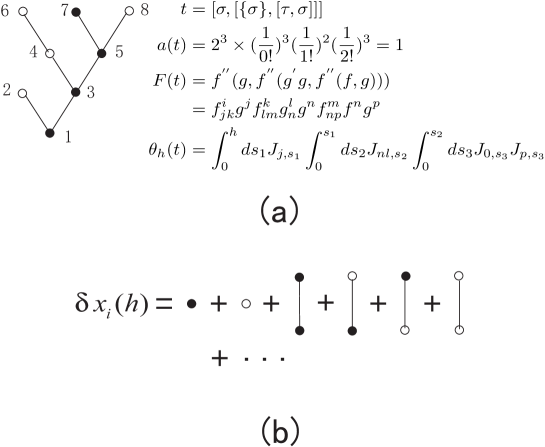
We will first introduce some useful notations [16]. Take the bicolour rooted tree t in Fig.1 as an example, The tree has 8 vertices, each vertex can be colored by white node (\circ) or black node (\bullet) which is the representative of stochastic node (σ𝜎\sigma) or deterministic node (τ𝜏\tau). If t1,,tmsubscript𝑡1subscript𝑡𝑚t_{1},\cdots,t_{m} are bicolour rooted trees, then [t1,,tm]subscript𝑡1subscript𝑡𝑚[t_{1},\cdots,t_{m}] and {t1,,tm}subscript𝑡1subscript𝑡𝑚\{t_{1},\cdots,t_{m}\} are trees in which t1,,tmsubscript𝑡1subscript𝑡𝑚t_{1},\cdots,t_{m} are each joined by a single branch to \bullet or \circ, respectively. We can therefore rewrite the tree t in a compact form [σ,[{σ},[τ,σ]]]𝜎𝜎𝜏𝜎[\sigma,[\{\sigma\},[\tau,\sigma]]]. To conveniently calculate the weight of this tree, we define the following terms: the degree of the vertex C(v)(vt)𝐶𝑣𝑣𝑡C(v)(v\in t) in the BRT is equivalent to the degree of vertex D(v)𝐷𝑣D(v) in the graph theory except the root 1 with C(1)=1+D(1)𝐶11𝐷1C(1)=1+D(1). S is the symmetry factor of the tree t, for example, the trees interchanged the branches joint to vertex 1 or 3 or 5 are regarded as identical with tree t, therefore the symmetry factor of tree t is 2×2×2=822282\times 2\times 2=8. Then tracing the stochastic Taylor expansion of the Eq.(7), we find that the elementary weight of the tree, which is also the coefficient of each term in the expansion, is

a(t)=Si=1n1(C(vi)1)!,𝑎𝑡𝑆superscriptsubscriptproduct𝑖1𝑛1𝐶subscript𝑣𝑖1a(t)=S\prod\limits_{i=1}^{n}\frac{1}{(C(v_{i})-1)!}, (11)

where n is the total number of vertex in the tree and vertex vitsubscript𝑣𝑖𝑡v_{i}\in t. Now we introduce the elementary derivative and elementary integral here [16]. An elementary derivative F(t)𝐹𝑡F(t) can be associated with a BRT such that

F(τ)=f,F(σ)=g,F(t)={f(m)[F(t1),,F(tm)],t=[t1,,tm]g(m)[F(t1),,F(tm)],t={t1,,tm},formulae-sequence𝐹𝜏𝑓formulae-sequence𝐹𝜎𝑔𝐹𝑡casessuperscript𝑓𝑚𝐹subscript𝑡1𝐹subscript𝑡𝑚𝑡subscript𝑡1subscript𝑡𝑚otherwisesuperscript𝑔𝑚𝐹subscript𝑡1𝐹subscript𝑡𝑚𝑡subscript𝑡1subscript𝑡𝑚otherwise\begin{split}&F(\tau)=f,F(\sigma)=g,\\ &F(t)=\begin{cases}f^{(m)}[F(t_{1}),\cdots,F(t_{m})],t=[t_{1},\cdots,t_{m}]\\ g^{(m)}[F(t_{1}),\cdots,F(t_{m})],t=\{t_{1},\cdots,t_{m}\},\end{cases}\end{split} (12)

and the elementary integral can be written as

θs(τ)=J0,s,θs(σ)=Ji,s,θs(t)={0s𝑑u(j=1mθu(tj)),t=[t1,,tm]0sdWi(u)(j=1mθu(tj)),t={t1,,tm}.formulae-sequencesubscript𝜃𝑠𝜏subscript𝐽0𝑠formulae-sequencesubscript𝜃𝑠𝜎subscript𝐽𝑖𝑠subscript𝜃𝑠𝑡casessuperscriptsubscript0𝑠differential-d𝑢superscriptsubscriptproduct𝑗1𝑚subscript𝜃𝑢subscript𝑡𝑗𝑡subscript𝑡1subscript𝑡𝑚otherwisesuperscriptsubscript0𝑠𝑑subscript𝑊𝑖𝑢superscriptsubscriptproduct𝑗1𝑚subscript𝜃𝑢subscript𝑡𝑗𝑡subscript𝑡1subscript𝑡𝑚otherwise\begin{split}&\theta_{s}(\tau)=J_{0,s},\theta_{s}(\sigma)=J_{i,s},\\ &\theta_{s}(t)=\begin{cases}\int_{0}^{s}du(\prod\limits_{j=1}^{m}\theta_{u}(t_{j})),t=[t_{1},\cdots,t_{m}]\\ \int_{0}^{s}\circ dW_{i}(u)(\prod\limits_{j=1}^{m}\theta_{u}(t_{j})),t=\{t_{1},\cdots,t_{m}\}.\end{cases}\end{split} (13)

Fig.1(a) illustrates the elementary weight, derivative and integral graphically.
Refer to caption

Figure 1: Illustration of the BRT method. Fig.1(a) shows a bicolour rooted tree t, and its elementary weight a(t)𝑎𝑡a(t), derivative F(t)𝐹𝑡F(t) and integral θh(t)subscript𝜃𝑡\theta_{h}(t), respectively. Fig.1(b) shows the 0th and 1st derivative terms of stochastic Taylor expansion of δxi(h)𝛿subscript𝑥𝑖\delta x_{i}(h) by the BRT method.

Therefore the stochastic Taylor expansion is given by

δxi(h)=tTa(t)F(t)θh(t)=sum of all the non-isomorphicbicolour rooted trees,𝛿subscript𝑥𝑖subscript𝑡𝑇𝑎𝑡𝐹𝑡subscript𝜃𝑡sum of all the non-isomorphicbicolour rooted trees\begin{split}\delta x_{i}(h)=&\sum\limits_{t\in T}a(t)F(t)\theta_{h}(t)\\ =&\textit{sum of all the non-isomorphic}\\ &\textit{bicolour rooted trees},\\ \end{split} (14)

where T is the set of non-isomorphic bicolour rooted trees. Fig.1(b) illustrates how to use this formula to express δxi(h)=δxi0(h)+δxi1(h)+𝛿subscript𝑥𝑖𝛿superscriptsubscript𝑥𝑖0𝛿superscriptsubscript𝑥𝑖1\delta x_{i}(h)=\delta x_{i}^{0}(h)+\delta x_{i}^{1}(h)+\cdots.

3 Algorithm

Due to the complexity of stochastic Taylor expansion, we only consider Langevin equation (LE) which plays an important part in the fields involving randomness in this paper. An N dimensional set of coupled LEs has the form

qi¨=V(q(t))qiγiqi˙+ξi(t),¨subscript𝑞𝑖𝑉q𝑡subscript𝑞𝑖subscript𝛾𝑖˙subscript𝑞𝑖subscript𝜉𝑖𝑡\ddot{q_{i}}=-\frac{\partial V(\textbf{q}(t))}{\partial q_{i}}-\gamma_{i}\dot{q_{i}}+\xi_{i}(t), (15)

where V(q(t))𝑉q𝑡V(\textbf{q}(t)) is the external potential, γi(i=1,,N)subscript𝛾𝑖𝑖1𝑁\gamma_{i}(i=1,\cdots,N) is a set of friction parameters, ξi(t)subscript𝜉𝑖𝑡\xi_{i}(t) is random noise with zero mean, the correlation relation is

<ξi(t)ξj(t)>=2γiTδijδ(tt),expectationsubscript𝜉𝑖𝑡subscript𝜉𝑗superscript𝑡2subscript𝛾𝑖𝑇subscript𝛿𝑖𝑗𝛿𝑡superscript𝑡<\xi_{i}(t)\xi_{j}(t^{{}^{\prime}})>=2\gamma_{i}T\delta_{ij}\delta(t-t^{{}^{\prime}}), (16)

and the Hamilton canonical equations are

qi˙=pi,pi˙=V(q(t))qiγipi+ξi(t).formulae-sequence˙subscript𝑞𝑖subscript𝑝𝑖˙subscript𝑝𝑖𝑉q𝑡subscript𝑞𝑖subscript𝛾𝑖subscript𝑝𝑖subscript𝜉𝑖𝑡\begin{split}&\dot{q_{i}}=p_{i},\\ &\dot{p_{i}}=-\frac{\partial V(\textbf{q}(t))}{\partial q_{i}}-\gamma_{i}p_{i}+\xi_{i}(t).\end{split} (17)

The form of Eq.(17) where only every second equation has a noise term with constant diffusion coefficient, as well as the potential V(q(t))𝑉q𝑡V(\textbf{q}(t)) is unrelated to p(t)p𝑡\textbf{p}(t), makes it possible to sharply decrease the complexity of Eq.(14) so as to obtain a high order algorithm for LE.

For the Eq.(17), we can translate it into the form

xi˙=fi(X(t))+giξi(t)(i=1,2,,2N)<ξi(t)ξj(t)>=δijδ(tt),formulae-sequence˙subscript𝑥𝑖subscript𝑓𝑖𝑋𝑡subscript𝑔𝑖subscript𝜉𝑖𝑡𝑖122𝑁expectationsubscript𝜉𝑖𝑡subscript𝜉𝑗superscript𝑡subscript𝛿𝑖𝑗𝛿𝑡superscript𝑡\begin{split}&\dot{x_{i}}=f_{i}(X(t))+g_{i}\xi_{i}(t)\ \ \ (i=1,2,...,2N)\\ &<\xi_{i}(t)\xi_{j}(t^{{}^{\prime}})>=\delta_{ij}\delta(t-t^{{}^{\prime}}),\end{split} (18)

where fi(X(t))subscript𝑓𝑖𝑋𝑡f_{i}(X(t)) is equal to xi+1subscript𝑥𝑖1x_{i+1} for odd i and to V(X(t))/xi1γixi𝑉X𝑡subscript𝑥𝑖1subscript𝛾𝑖subscript𝑥𝑖-\partial V(\textbf{X}(t))/\partial x_{i-1}-\gamma_{i}x_{i} for even i, X(t)={x1,x3,,x2N1}X𝑡subscript𝑥1subscript𝑥3subscript𝑥2𝑁1\textbf{X}(t)=\{x_{1},x_{3},...,x_{2N-1}\}, gisubscript𝑔𝑖g_{i} is a set of constants with gi=0subscript𝑔𝑖0g_{i}=0 if i is odd number. Because of the property of V(q(t))𝑉q𝑡V(\textbf{q}(t)), one can find that fjki0superscriptsubscript𝑓𝑗𝑘𝑖0f_{jk}^{i}\neq 0 only if j and k are both odd numbers. From above properties, a key property for the simplification of the stochastic Taylor expansion, that is, fjkigj=0superscriptsubscript𝑓𝑗𝑘𝑖subscript𝑔𝑗0\cdots f_{jk}^{i}g_{j}\cdots=0, can be found. We can rewrite it in the compact form as follow:

,[,σ,],=0,𝜎0\cdots,[\cdots,\sigma,\cdots],\cdots=0, (19)

so if a bicolour rooted tree has this structure, it should have no contribution to the stochastic Taylor expansion.

From the analysis above, one can obtain a general method for solving the Langevin equation numerically. If we want to get a numerical method to the order o(m,n), we should:

(a)For the deterministic part:

Solve it by the standard Runge-Kutta method of order m.

(b)For the stochastic part:

(i)Write down all the non-isomorphic bicolour rooted trees that can avoid the structure (19);

(ii)Attach each vertex with white or black so as to make the tree have order n.

(c)Add up the results of (a) and (b).

Using these three criteria, all the terms up to order o(7,4.5) are,

δxidet(h)=j=06RK(j),δxiran(h)=σ+[σ]+[[σ]]+[[[σ]]]+[τ,[σ]]+[[[[σ]]]]+[τ,[[σ]]]+[[τ],[σ]]+[τ,τ,[σ]]+[[τ,[σ]]]+[[σ],[σ]],δxi(h)=δxidet(h)+δxiran(h).formulae-sequence𝛿subscript𝑥𝑖𝑑𝑒𝑡superscriptsubscript𝑗06𝑅𝐾𝑗formulae-sequence𝛿subscript𝑥𝑖𝑟𝑎𝑛𝜎delimited-[]𝜎delimited-[]delimited-[]𝜎delimited-[]delimited-[]delimited-[]𝜎𝜏delimited-[]𝜎delimited-[]delimited-[]delimited-[]delimited-[]𝜎𝜏delimited-[]delimited-[]𝜎delimited-[]𝜏delimited-[]𝜎𝜏𝜏delimited-[]𝜎delimited-[]𝜏delimited-[]𝜎delimited-[]𝜎delimited-[]𝜎𝛿subscript𝑥𝑖𝛿subscript𝑥𝑖𝑑𝑒𝑡𝛿subscript𝑥𝑖𝑟𝑎𝑛\begin{split}\delta x_{idet}(h)=&\sum\limits_{j=0}^{6}RK(j),\\ \delta x_{iran}(h)=&\sigma+[\sigma]+[[\sigma]]+[[[\sigma]]]+[\tau,[\sigma]]\\ &+[[[[\sigma]]]]+[\tau,[[\sigma]]]+[[\tau],[\sigma]]\\ &+[\tau,\tau,[\sigma]]+[[\tau,[\sigma]]]+[[\sigma],[\sigma]],\\ \delta x_{i}(h)=&\delta x_{idet}(h)+\delta x_{iran}(h).\\ \end{split} (20)

where the RK(j),(j=0,,6)𝑅𝐾𝑗𝑗06RK(j),(j=0,\cdots,6) are the BRTs with j+1𝑗1j+1 deterministic nodes only which are identical to the terms of standard Runge-Kutta method for ODEs. These terms compose the deterministic part of our algorithm, and we can use Runge-Kutta method to solve the deterministic part numerically [17, 19].

Then we try to find a way to calculate the stochastic part in Eq.(20). We here introduce a method to approximate the elementary integral which is developed by P. E. Kloeden and E. Platen [18]. They showed that if W(t)=(W1(t),,WN(t))W𝑡subscript𝑊1𝑡subscript𝑊𝑁𝑡\textbf{W}(t)=(W_{1}(t),\cdots,W_{N}(t)) is an N-dimensional Wiener process on the time interval [0,h]0[0,h], the componentwise Fourier expansion of the Brownian bridge process W(t)thW(h)W𝑡𝑡W\textbf{W}(t)-\frac{t}{h}\textbf{W}(h) is

Wi(t)thWi(h)=12ai0+j=1(aijcos(2jπth)+bijsin(2jπth)),subscript𝑊𝑖𝑡𝑡subscript𝑊𝑖12subscript𝑎𝑖0superscriptsubscript𝑗1subscript𝑎𝑖𝑗2𝑗𝜋𝑡subscript𝑏𝑖𝑗2𝑗𝜋𝑡W_{i}(t)-\frac{t}{h}W_{i}(h)=\frac{1}{2}a_{i0}+\sum\limits_{j=1}^{\infty}(a_{ij}\cos(\frac{2j\pi t}{h})+b_{ij}\sin(\frac{2j\pi t}{h})), (21)

where aij,bijsubscript𝑎𝑖𝑗subscript𝑏𝑖𝑗a_{ij},b_{ij} are N(0,h/2π2j2)𝑁02superscript𝜋2superscript𝑗2N(0,h/2\pi^{2}j^{2}) distributed and pairwise independent, then setting t=0𝑡0t=0 in the equation (21) gives ai0=2j=1aijai0subscript𝑎𝑖02superscriptsubscript𝑗1subscript𝑎𝑖𝑗superscriptsubscript𝑎𝑖0a_{i0}=-2\sum\limits_{j=1}^{\infty}a_{ij}\equiv a_{i}^{0}.

Now, we begin to calculate the stochastic part of Eq.(20). Firstly, let us set the W(0)=0W00\textbf{W}(0)=0, then use equation (21), we can easily find that

σ=a(σ)F(σ)θh(σ)=giJi,h=giWi(h)giωi1,[σ]=fjigjJj0,h=fjigj0h𝑑s10s1𝑑Wj(s2)=fjigj0hWj(s1)𝑑s1=hfjigj(Wj(h)2+aj02)hfjigjωj2,formulae-sequence𝜎𝑎𝜎𝐹𝜎subscript𝜃𝜎superscript𝑔𝑖subscript𝐽𝑖superscript𝑔𝑖subscript𝑊𝑖superscript𝑔𝑖superscriptsubscript𝜔𝑖1delimited-[]𝜎superscriptsubscript𝑓𝑗𝑖superscript𝑔𝑗subscript𝐽𝑗0superscriptsubscript𝑓𝑗𝑖superscript𝑔𝑗superscriptsubscript0differential-dsubscript𝑠1superscriptsubscript0subscript𝑠1differential-dsubscript𝑊𝑗subscript𝑠2superscriptsubscript𝑓𝑗𝑖superscript𝑔𝑗superscriptsubscript0subscript𝑊𝑗subscript𝑠1differential-dsubscript𝑠1superscriptsubscript𝑓𝑗𝑖superscript𝑔𝑗subscript𝑊𝑗2superscriptsubscript𝑎𝑗02superscriptsubscript𝑓𝑗𝑖superscript𝑔𝑗superscriptsubscript𝜔𝑗2\begin{split}\sigma&=a(\sigma)F(\sigma)\theta_{h}(\sigma)=g^{i}J_{i,h}=g^{i}W_{i}(h)\equiv g^{i}\omega_{i}^{1},\\ [\sigma]&=f_{j}^{i}g^{j}J_{j0,h}=f_{j}^{i}g^{j}\int_{0}^{h}ds_{1}\int_{0}^{s_{1}}\circ dW_{j}(s_{2})\\ &=f_{j}^{i}g^{j}\int_{0}^{h}W_{j}(s_{1})ds_{1}\\ &=hf_{j}^{i}g^{j}(\frac{W_{j}(h)}{2}+\frac{a_{j}^{0}}{2})\\ &\equiv hf_{j}^{i}g^{j}\omega_{j}^{2},\\ \end{split} (22)

where Wi(h)Wisubscript𝑊𝑖subscript𝑊𝑖W_{i}(h)\equiv W_{i} is a set of independent Gaussian random variables sampled from N(0,h)𝑁0N(0,h). Similarly calculation gives

[[σ]]=h2fjifkjgkωk3[[[σ]]]=h3fjifkjflkglωl4[τ,[σ]]=h3fjkifjflkglωl5[[[[σ]]]]=h4fjifkjflkfmlgmωm6[τ,[[σ]]]=h4fjkifjflkfmlgmωm7[[τ],[σ]]=h4fjkifljflfmkgmωm8[τ,τ,[σ]]=h42fjklifjfkfmlgmωm9[[τ,[σ]]]=h4fjifkljfkfmlgmωm10[[σ],[σ]]=h32fjkifljglfmkgmΩlm1delimited-[]delimited-[]𝜎superscript2superscriptsubscript𝑓𝑗𝑖superscriptsubscript𝑓𝑘𝑗superscript𝑔𝑘superscriptsubscript𝜔𝑘3delimited-[]delimited-[]delimited-[]𝜎superscript3superscriptsubscript𝑓𝑗𝑖superscriptsubscript𝑓𝑘𝑗superscriptsubscript𝑓𝑙𝑘superscript𝑔𝑙superscriptsubscript𝜔𝑙4𝜏delimited-[]𝜎superscript3superscriptsubscript𝑓𝑗𝑘𝑖superscript𝑓𝑗superscriptsubscript𝑓𝑙𝑘superscript𝑔𝑙superscriptsubscript𝜔𝑙5delimited-[]delimited-[]delimited-[]delimited-[]𝜎superscript4superscriptsubscript𝑓𝑗𝑖superscriptsubscript𝑓𝑘𝑗superscriptsubscript𝑓𝑙𝑘superscriptsubscript𝑓𝑚𝑙superscript𝑔𝑚superscriptsubscript𝜔𝑚6𝜏delimited-[]delimited-[]𝜎superscript4superscriptsubscript𝑓𝑗𝑘𝑖superscript𝑓𝑗superscriptsubscript𝑓𝑙𝑘superscriptsubscript𝑓𝑚𝑙superscript𝑔𝑚superscriptsubscript𝜔𝑚7delimited-[]𝜏delimited-[]𝜎superscript4superscriptsubscript𝑓𝑗𝑘𝑖superscriptsubscript𝑓𝑙𝑗superscript𝑓𝑙superscriptsubscript𝑓𝑚𝑘superscript𝑔𝑚superscriptsubscript𝜔𝑚8𝜏𝜏delimited-[]𝜎superscript42superscriptsubscript𝑓𝑗𝑘𝑙𝑖superscript𝑓𝑗superscript𝑓𝑘superscriptsubscript𝑓𝑚𝑙superscript𝑔𝑚superscriptsubscript𝜔𝑚9delimited-[]𝜏delimited-[]𝜎superscript4superscriptsubscript𝑓𝑗𝑖superscriptsubscript𝑓𝑘𝑙𝑗superscript𝑓𝑘superscriptsubscript𝑓𝑚𝑙superscript𝑔𝑚superscriptsubscript𝜔𝑚10delimited-[]𝜎delimited-[]𝜎superscript32superscriptsubscript𝑓𝑗𝑘𝑖superscriptsubscript𝑓𝑙𝑗superscript𝑔𝑙superscriptsubscript𝑓𝑚𝑘superscript𝑔𝑚superscriptsubscriptΩ𝑙𝑚1\begin{split}[[\sigma]]&=h^{2}f_{j}^{i}f_{k}^{j}g^{k}\omega_{k}^{3}\\ [[[\sigma]]]&=h^{3}f_{j}^{i}f_{k}^{j}f_{l}^{k}g^{l}\omega_{l}^{4}\\ [\tau,[\sigma]]&=h^{3}f_{jk}^{i}f^{j}f_{l}^{k}g^{l}\omega_{l}^{5}\\ [[[[\sigma]]]]&=h^{4}f_{j}^{i}f_{k}^{j}f_{l}^{k}f_{m}^{l}g^{m}\omega_{m}^{6}\\ [\tau,[[\sigma]]]&=h^{4}f_{jk}^{i}f^{j}f_{l}^{k}f_{m}^{l}g^{m}\omega_{m}^{7}\\ [[\tau],[\sigma]]&=h^{4}f_{jk}^{i}f_{l}^{j}f^{l}f_{m}^{k}g^{m}\omega_{m}^{8}\\ [\tau,\tau,[\sigma]]&=\frac{h^{4}}{2}f_{jkl}^{i}f^{j}f^{k}f_{m}^{l}g^{m}\omega_{m}^{9}\\ [[\tau,[\sigma]]]&=h^{4}f_{j}^{i}f_{kl}^{j}f^{k}f_{m}^{l}g^{m}\omega_{m}^{10}\\ [[\sigma],[\sigma]]&=\frac{h^{3}}{2}f_{jk}^{i}f_{l}^{j}g^{l}f_{m}^{k}g^{m}\Omega_{lm}^{1}\\ \end{split} (23)

where

ωi3=Wi6+ai04+bi12ωi4=Wi24+ai012+ai14+bi14ωi5=Wi8+ai06ai14+bi14ωi6=Wi120+ai048+ai18+bi112bi28ωi7=Wi30+ai016+ai18+bi16+bi28ωi8=Wi20+ai016ai18+bi112bi28ωi9=Wi10+ai08ai14+bi16bi24ωi10=Wi40+ai024+bi112+bi24ai0=2j=1aij,bi1=j=11πjbij,ai1=j=11(πj)2aij,bi2=j=11(πj)3bij,formulae-sequencesuperscriptsubscript𝜔𝑖3subscript𝑊𝑖6superscriptsubscript𝑎𝑖04superscriptsubscript𝑏𝑖12superscriptsubscript𝜔𝑖4subscript𝑊𝑖24superscriptsubscript𝑎𝑖012superscriptsubscript𝑎𝑖14superscriptsubscript𝑏𝑖14superscriptsubscript𝜔𝑖5subscript𝑊𝑖8superscriptsubscript𝑎𝑖06superscriptsubscript𝑎𝑖14superscriptsubscript𝑏𝑖14superscriptsubscript𝜔𝑖6subscript𝑊𝑖120superscriptsubscript𝑎𝑖048superscriptsubscript𝑎𝑖18superscriptsubscript𝑏𝑖112superscriptsubscript𝑏𝑖28superscriptsubscript𝜔𝑖7subscript𝑊𝑖30superscriptsubscript𝑎𝑖016superscriptsubscript𝑎𝑖18superscriptsubscript𝑏𝑖16superscriptsubscript𝑏𝑖28superscriptsubscript𝜔𝑖8subscript𝑊𝑖20superscriptsubscript𝑎𝑖016superscriptsubscript𝑎𝑖18superscriptsubscript𝑏𝑖112superscriptsubscript𝑏𝑖28superscriptsubscript𝜔𝑖9subscript𝑊𝑖10superscriptsubscript𝑎𝑖08superscriptsubscript𝑎𝑖14superscriptsubscript𝑏𝑖16superscriptsubscript𝑏𝑖24superscriptsubscript𝜔𝑖10subscript𝑊𝑖40superscriptsubscript𝑎𝑖024superscriptsubscript𝑏𝑖112superscriptsubscript𝑏𝑖24superscriptsubscript𝑎𝑖02superscriptsubscript𝑗1subscript𝑎𝑖𝑗formulae-sequencesuperscriptsubscript𝑏𝑖1superscriptsubscript𝑗11𝜋𝑗subscript𝑏𝑖𝑗formulae-sequencesuperscriptsubscript𝑎𝑖1superscriptsubscript𝑗11superscript𝜋𝑗2subscript𝑎𝑖𝑗superscriptsubscript𝑏𝑖2superscriptsubscript𝑗11superscript𝜋𝑗3subscript𝑏𝑖𝑗\begin{split}\omega_{i}^{3}&=\frac{W_{i}}{6}+\frac{a_{i}^{0}}{4}+\frac{b_{i}^{1}}{2}\\ \omega_{i}^{4}&=\frac{W_{i}}{24}+\frac{a_{i}^{0}}{12}+\frac{a_{i}^{1}}{4}+\frac{b_{i}^{1}}{4}\\ \omega_{i}^{5}&=\frac{W_{i}}{8}+\frac{a_{i}^{0}}{6}-\frac{a_{i}^{1}}{4}+\frac{b_{i}^{1}}{4}\\ \omega_{i}^{6}&=\frac{W_{i}}{120}+\frac{a_{i}^{0}}{48}+\frac{a_{i}^{1}}{8}+\frac{b_{i}^{1}}{12}-\frac{b_{i}^{2}}{8}\\ \omega_{i}^{7}&=\frac{W_{i}}{30}+\frac{a_{i}^{0}}{16}+\frac{a_{i}^{1}}{8}+\frac{b_{i}^{1}}{6}+\frac{b_{i}^{2}}{8}\\ \omega_{i}^{8}&=\frac{W_{i}}{20}+\frac{a_{i}^{0}}{16}-\frac{a_{i}^{1}}{8}+\frac{b_{i}^{1}}{12}-\frac{b_{i}^{2}}{8}\\ \omega_{i}^{9}&=\frac{W_{i}}{10}+\frac{a_{i}^{0}}{8}-\frac{a_{i}^{1}}{4}+\frac{b_{i}^{1}}{6}-\frac{b_{i}^{2}}{4}\\ \omega_{i}^{10}&=\frac{W_{i}}{40}+\frac{a_{i}^{0}}{24}+\frac{b_{i}^{1}}{12}+\frac{b_{i}^{2}}{4}\\ a_{i}^{0}&=-2\sum\limits_{j=1}^{\infty}a_{ij},\ b_{i}^{1}=\sum\limits_{j=1}^{\infty}\frac{1}{\pi j}b_{ij},\\ a_{i}^{1}&=\sum\limits_{j=1}^{\infty}\frac{1}{(\pi j)^{2}}a_{ij},\ b_{i}^{2}=\sum\limits_{j=1}^{\infty}\frac{1}{(\pi j)^{3}}b_{ij},\\ \end{split} (24)

and the first non-Gaussian random variable is

Ωij1=ωi1ωj9+ai0ωj5ωi1ωj120ai0aj012ai0ωj18+bi1bj14+cij8,cij=k=11(πk)2(aikajk+bikbjk).formulae-sequencesuperscriptsubscriptΩ𝑖𝑗1superscriptsubscript𝜔𝑖1superscriptsubscript𝜔𝑗9superscriptsubscript𝑎𝑖0superscriptsubscript𝜔𝑗5superscriptsubscript𝜔𝑖1superscriptsubscript𝜔𝑗120superscriptsubscript𝑎𝑖0superscriptsubscript𝑎𝑗012superscriptsubscript𝑎𝑖0superscriptsubscript𝜔𝑗18superscriptsubscript𝑏𝑖1superscriptsubscript𝑏𝑗14subscript𝑐𝑖𝑗8subscript𝑐𝑖𝑗superscriptsubscript𝑘11superscript𝜋𝑘2subscript𝑎𝑖𝑘subscript𝑎𝑗𝑘subscript𝑏𝑖𝑘subscript𝑏𝑗𝑘\begin{split}\Omega_{ij}^{1}&=\omega_{i}^{1}\omega_{j}^{9}+a_{i}^{0}\omega_{j}^{5}-\frac{\omega_{i}^{1}\omega_{j}^{1}}{20}-\frac{a_{i}^{0}a_{j}^{0}}{12}-\frac{a_{i}^{0}\omega_{j}^{1}}{8}+\frac{b_{i}^{1}b_{j}^{1}}{4}+\frac{c_{ij}}{8},\\ c_{ij}&=\sum\limits_{k=1}^{\infty}\frac{1}{(\pi k)^{2}}(a_{ik}a_{jk}+b_{ik}b_{jk}).\\ \end{split} (25)

We can find that there are only 5 independent variables among ωij,(j=1,,10)superscriptsubscript𝜔𝑖𝑗𝑗110\omega_{i}^{j},(j=1,\cdots,10). Let’s choose ωi1,ωi2,ωi3,ωi4,ωi6superscriptsubscript𝜔𝑖1superscriptsubscript𝜔𝑖2superscriptsubscript𝜔𝑖3superscriptsubscript𝜔𝑖4superscriptsubscript𝜔𝑖6\omega_{i}^{1},\omega_{i}^{2},\omega_{i}^{3},\omega_{i}^{4},\omega_{i}^{6} as the independent variables, then

ωi5=ωi3ωi4ωi7=ωi4ωi6ωi8=12ωi3ωi4+ωi6ωi9=ωi32ωi4+2ωi6ωi10=ωi42ωi6superscriptsubscript𝜔𝑖5superscriptsubscript𝜔𝑖3superscriptsubscript𝜔𝑖4superscriptsubscript𝜔𝑖7superscriptsubscript𝜔𝑖4superscriptsubscript𝜔𝑖6superscriptsubscript𝜔𝑖812superscriptsubscript𝜔𝑖3superscriptsubscript𝜔𝑖4superscriptsubscript𝜔𝑖6superscriptsubscript𝜔𝑖9superscriptsubscript𝜔𝑖32superscriptsubscript𝜔𝑖42superscriptsubscript𝜔𝑖6superscriptsubscript𝜔𝑖10superscriptsubscript𝜔𝑖42superscriptsubscript𝜔𝑖6\begin{split}\omega_{i}^{5}&=\omega_{i}^{3}-\omega_{i}^{4}\\ \omega_{i}^{7}&=\omega_{i}^{4}-\omega_{i}^{6}\\ \omega_{i}^{8}&=\frac{1}{2}\omega_{i}^{3}-\omega_{i}^{4}+\omega_{i}^{6}\\ \omega_{i}^{9}&=\omega_{i}^{3}-2\omega_{i}^{4}+2\omega_{i}^{6}\\ \omega_{i}^{10}&=\omega_{i}^{4}-2\omega_{i}^{6}\end{split} (26)

Now, the last procedure we should do is to determine the five Gaussian random variables Wi,ai0,ai1,bi1,bi2subscript𝑊𝑖superscriptsubscript𝑎𝑖0superscriptsubscript𝑎𝑖1superscriptsubscript𝑏𝑖1superscriptsubscript𝑏𝑖2W_{i},a_{i}^{0},a_{i}^{1},b_{i}^{1},b_{i}^{2} and the non-Gaussian random variable cijsubscript𝑐𝑖𝑗c_{ij}. We truncate cijsubscript𝑐𝑖𝑗c_{ij} to the first term, that is, cij(ai1aj1+bi1bj1)/π2subscript𝑐𝑖𝑗subscript𝑎𝑖1subscript𝑎𝑗1subscript𝑏𝑖1subscript𝑏𝑗1superscript𝜋2c_{ij}\approx(a_{i1}a_{j1}+b_{i1}b_{j1})/\pi^{2}. Since Wi,aij,bijsubscript𝑊𝑖subscript𝑎𝑖𝑗subscript𝑏𝑖𝑗W_{i},a_{ij},b_{ij} are independent and WiN(0,h),aijN(0,h/2π2j2),bijN(0,h/2π2j2)formulae-sequencesimilar-tosubscript𝑊𝑖𝑁0formulae-sequencesimilar-tosubscript𝑎𝑖𝑗𝑁02superscript𝜋2superscript𝑗2similar-tosubscript𝑏𝑖𝑗𝑁02superscript𝜋2superscript𝑗2W_{i}\sim N(0,h),\ a_{ij}\sim N(0,h/2\pi^{2}j^{2}),\ b_{ij}\sim N(0,h/2\pi^{2}j^{2}), we can see that

ai0N(0,h3),bi1N(0,h180),ai1N(0,h1890),bi2N(0,h18900),<ai0ai1>=h90,<ai0ai1>=hπ2,<ai1ai1>=h2π4,<bi1bi2>=h1890,<bi1bi1>=h2π3,<bi2bi1>=h2π5.formulae-sequencesimilar-tosuperscriptsubscript𝑎𝑖0𝑁03formulae-sequencesimilar-tosuperscriptsubscript𝑏𝑖1𝑁0180formulae-sequencesimilar-tosuperscriptsubscript𝑎𝑖1𝑁01890formulae-sequencesimilar-tosuperscriptsubscript𝑏𝑖2𝑁018900formulae-sequenceMissing Operatorformulae-sequenceexpectationsuperscriptsubscript𝑎𝑖0subscript𝑎𝑖1superscript𝜋2formulae-sequenceexpectationsuperscriptsubscript𝑎𝑖1subscript𝑎𝑖12superscript𝜋4formulae-sequenceMissing Operatorformulae-sequenceexpectationsuperscriptsubscript𝑏𝑖1subscript𝑏𝑖12superscript𝜋3expectationsuperscriptsubscript𝑏𝑖2subscript𝑏𝑖12superscript𝜋5\begin{split}a_{i}^{0}\sim&N(0,\frac{h}{3}),\ b_{i}^{1}\sim N(0,\frac{h}{180}),\\ a_{i}^{1}\sim&N(0,\frac{h}{1890}),\ b_{i}^{2}\sim N(0,\frac{h}{18900}),\\ <a_{i}^{0}&a_{i}^{1}>=-\frac{h}{90},\ <a_{i}^{0}a_{i1}>=-\frac{h}{\pi^{2}},\ <a_{i}^{1}a_{i1}>=\frac{h}{2\pi^{4}},\\ <b_{i}^{1}&b_{i}^{2}>=\frac{h}{1890},\ <b_{i}^{1}b_{i1}>=\frac{h}{2\pi^{3}},\ <b_{i}^{2}b_{i1}>=\frac{h}{2\pi^{5}}.\\ \end{split} (27)

Let ϕi1,ϕi2,ϕi3,ϕi4,ϕi5,ϕi6,ϕi7superscriptsubscriptitalic-ϕ𝑖1superscriptsubscriptitalic-ϕ𝑖2superscriptsubscriptitalic-ϕ𝑖3superscriptsubscriptitalic-ϕ𝑖4superscriptsubscriptitalic-ϕ𝑖5superscriptsubscriptitalic-ϕ𝑖6superscriptsubscriptitalic-ϕ𝑖7\phi_{i}^{1},\phi_{i}^{2},\phi_{i}^{3},\phi_{i}^{4},\phi_{i}^{5},\phi_{i}^{6},\phi_{i}^{7} to be seven independent standard Gaussian random variables, then use Eq.(27), we can get

Wi=hϕi1ai0=h3ϕi2ai1=h30(ϕi23+ϕi37)bi1=h180ϕi4bi2=h63(ϕi45+ϕi510)ai1=h(0.175493ϕi2+0.139348ϕi3+0.0210906ϕi6)bi1=h(0.21635ϕi4+0.0617995ϕi5+0.00584342ϕi7)subscript𝑊𝑖superscriptsubscriptitalic-ϕ𝑖1superscriptsubscript𝑎𝑖03superscriptsubscriptitalic-ϕ𝑖2superscriptsubscript𝑎𝑖130superscriptsubscriptitalic-ϕ𝑖23superscriptsubscriptitalic-ϕ𝑖37superscriptsubscript𝑏𝑖1180superscriptsubscriptitalic-ϕ𝑖4superscriptsubscript𝑏𝑖263superscriptsubscriptitalic-ϕ𝑖45superscriptsubscriptitalic-ϕ𝑖510subscript𝑎𝑖10.175493superscriptsubscriptitalic-ϕ𝑖20.139348superscriptsubscriptitalic-ϕ𝑖30.0210906superscriptsubscriptitalic-ϕ𝑖6subscript𝑏𝑖10.21635superscriptsubscriptitalic-ϕ𝑖40.0617995superscriptsubscriptitalic-ϕ𝑖50.00584342superscriptsubscriptitalic-ϕ𝑖7\begin{split}W_{i}&=\sqrt{h}\phi_{i}^{1}\\ a_{i}^{0}&=\sqrt{\frac{h}{3}}\phi_{i}^{2}\\ a_{i}^{1}&=\frac{\sqrt{h}}{30}(-\frac{\phi_{i}^{2}}{\sqrt{3}}+\frac{\phi_{i}^{3}}{\sqrt{7}})\\ b_{i}^{1}&=\sqrt{\frac{h}{180}}\phi_{i}^{4}\\ b_{i}^{2}&=\frac{\sqrt{h}}{63}(\frac{\phi_{i}^{4}}{\sqrt{5}}+\frac{\phi_{i}^{5}}{10})\\ a_{i1}&=\sqrt{h}(-0.175493\phi_{i}^{2}+0.139348\phi_{i}^{3}+0.0210906\phi_{i}^{6})\\ b_{i1}&=\sqrt{h}(0.21635\phi_{i}^{4}+0.0617995\phi_{i}^{5}+0.00584342\phi_{i}^{7})\\ \end{split} (28)

The BRT method gives an algorithm for the Langevin equation so long as we determine the deterministic and the stochastic part of Eq.(20) respectively and add up each other. The deterministic part can be solved by the standard Runge-Kutta algorithm [19], and the stochastic part can be solved by the Eqs.(22)-(23).

4 Numerical simulations

4.1 Energy relaxation in double well

To verify the validity of our algorithm, the Kramers equation will be considered as the severe test for our algorithm. The form is as follow:

q˙(t)=p(t),p˙(t)=V(q(t))γp(t)+ξ(t),formulae-sequence˙𝑞𝑡𝑝𝑡˙𝑝𝑡superscript𝑉𝑞𝑡𝛾𝑝𝑡𝜉𝑡\begin{split}\dot{q}(t)&=p(t),\\ \dot{p}(t)&=-V^{{}^{\prime}}(q(t))-\gamma p(t)+\xi(t),\\ \end{split} (29)

and ξ(t)𝜉𝑡\xi(t) is the Gaussian random force obeying the fluctuation dissipation theorem

<ξ(t)ξ(t)>=2γT.expectation𝜉𝑡𝜉superscript𝑡2𝛾𝑇<\xi(t)\xi(t^{{}^{\prime}})>=2\gamma T. (30)

Our method implies that the algorithm for Eqs.(29)-(30) is,

q(t+h)=qdet(q(t),p(t),h)+qran(q(t),p(t),h),p(t+h)=pdet(q(t),p(t),h)+pran(q(t),p(t),h),formulae-sequence𝑞𝑡subscript𝑞𝑑𝑒𝑡𝑞𝑡𝑝𝑡subscript𝑞𝑟𝑎𝑛𝑞𝑡𝑝𝑡𝑝𝑡subscript𝑝𝑑𝑒𝑡𝑞𝑡𝑝𝑡subscript𝑝𝑟𝑎𝑛𝑞𝑡𝑝𝑡\begin{split}q(t+h)=&q_{det}(q(t),p(t),h)+q_{ran}(q(t),p(t),h),\\ p(t+h)=&p_{det}(q(t),p(t),h)+p_{ran}(q(t),p(t),h),\\ \end{split} (31)

where qdet(q(t),p(t),h)subscript𝑞𝑑𝑒𝑡𝑞𝑡𝑝𝑡q_{det}(q(t),p(t),h) and pdet(q(t),p(t),h)subscript𝑝𝑑𝑒𝑡𝑞𝑡𝑝𝑡p_{det}(q(t),p(t),h) are the results of evolving the equations in the period 0-h by the seventh-order Runge-Kutta algorithm [19] which is used in the ODE, and the stochastic part of Eq.(31) is,

qran(q(t),p(t),h)=2γT[(hω22h2γω23+h3γ2ω24h4γ3ω26)+(h3ω24+2h4γω26)V′′h4p(t)ω210V′′′],pran(q(t),p(t),h)=2γT[(ω21hγω22+h2γ2ω23h3γ3ω24+h4γ4ω26)+(h2ω23+2h3γω243h4γ2ω26)V′′+(h3p(t)ω25+h4γp(t)ω27+h4γp(t)ω28+h4γp(t)ω210)V′′′+h4V′′V′′ω26+h4VV′′′ω28h42V′′′′p2(t)ω29]h3γTV′′′Ω221,formulae-sequencesubscript𝑞𝑟𝑎𝑛𝑞𝑡𝑝𝑡2𝛾𝑇delimited-[]superscriptsubscript𝜔22superscript2𝛾superscriptsubscript𝜔23superscript3superscript𝛾2superscriptsubscript𝜔24superscript4superscript𝛾3superscriptsubscript𝜔26superscript3superscriptsubscript𝜔242superscript4𝛾superscriptsubscript𝜔26superscript𝑉′′superscript4𝑝𝑡superscriptsubscript𝜔210superscript𝑉′′′subscript𝑝𝑟𝑎𝑛𝑞𝑡𝑝𝑡2𝛾𝑇delimited-[]superscriptsubscript𝜔21𝛾superscriptsubscript𝜔22superscript2superscript𝛾2superscriptsubscript𝜔23superscript3superscript𝛾3superscriptsubscript𝜔24superscript4superscript𝛾4superscriptsubscript𝜔26superscript2superscriptsubscript𝜔232superscript3𝛾superscriptsubscript𝜔243superscript4superscript𝛾2superscriptsubscript𝜔26superscript𝑉′′superscript3𝑝𝑡superscriptsubscript𝜔25superscript4𝛾𝑝𝑡superscriptsubscript𝜔27superscript4𝛾𝑝𝑡superscriptsubscript𝜔28superscript4𝛾𝑝𝑡superscriptsubscript𝜔210superscript𝑉′′′superscript4superscript𝑉′′superscript𝑉′′superscriptsubscript𝜔26superscript4superscript𝑉superscript𝑉′′′superscriptsubscript𝜔28superscript42superscript𝑉′′′′superscript𝑝2𝑡superscriptsubscript𝜔29superscript3𝛾𝑇superscript𝑉′′′superscriptsubscriptΩ221\begin{split}q_{ran}(q(t),p(t),h)=&\sqrt{2\gamma T}[(h\omega_{2}^{2}-h^{2}\gamma\omega_{2}^{3}+h^{3}\gamma^{2}\omega_{2}^{4}-h^{4}\gamma^{3}\omega_{2}^{6})\\ +&(-h^{3}\omega_{2}^{4}+2h^{4}\gamma\omega_{2}^{6})V^{{}^{\prime\prime}}-h^{4}p(t)\omega_{2}^{10}V^{{}^{\prime\prime\prime}}],\\ p_{ran}(q(t),p(t),h)=&\sqrt{2\gamma T}[(\omega_{2}^{1}-h\gamma\omega_{2}^{2}+h^{2}\gamma^{2}\omega_{2}^{3}-h^{3}\gamma^{3}\omega_{2}^{4}\\ +&h^{4}\gamma^{4}\omega_{2}^{6})+(-h^{2}\omega_{2}^{3}+2h^{3}\gamma\omega_{2}^{4}-3h^{4}\gamma^{2}\omega_{2}^{6})V^{{}^{\prime\prime}}\\ +&(-h^{3}p(t)\omega_{2}^{5}+h^{4}\gamma p(t)\omega_{2}^{7}+h^{4}\gamma p(t)\omega_{2}^{8}\\ +&h^{4}\gamma p(t)\omega_{2}^{10})V^{{}^{\prime\prime\prime}}+h^{4}V^{{}^{\prime\prime}}V^{{}^{\prime\prime}}\omega_{2}^{6}+h^{4}V^{{}^{\prime}}V^{{}^{\prime\prime\prime}}\omega_{2}^{8}\\ -&\frac{h^{4}}{2}V^{{}^{\prime\prime\prime\prime}}p^{2}(t)\omega_{2}^{9}]-h^{3}\gamma TV^{{}^{\prime\prime\prime}}\Omega_{22}^{1},\end{split} (32)

where ω2i(i=1,,10)superscriptsubscript𝜔2𝑖𝑖110\omega_{2}^{i}(i=1,\cdots,10) and Ω221superscriptsubscriptΩ221\Omega_{22}^{1} have been defined in the previous section.

The double well potential in this example is,

V(q)=q42q2.𝑉𝑞superscript𝑞42superscript𝑞2V(q)=q^{4}-2q^{2}. (33)

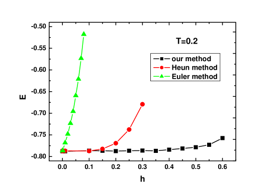
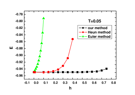
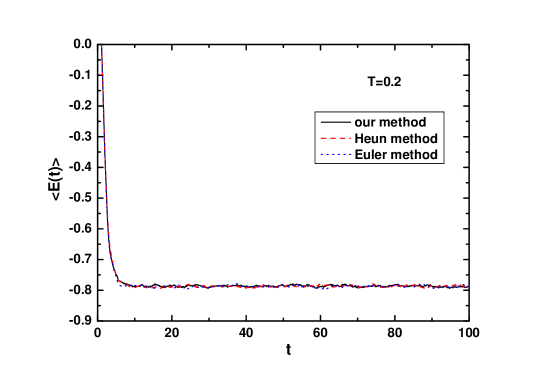
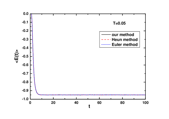
It has two minima located at q=±1𝑞plus-or-minus1q=\pm 1 and a potential barrier with the height ΔV=1Δ𝑉1\Delta V=1 between the two wells. The friction coefficient γ𝛾\gamma is set to 1. The initial condition is chosen on the top of the barrier. The average is taken over 5000 realizations of the Gaussian random force during the trajectory. Fig.2 shows the result which is compared with the Euler method and the Heun method [20]. We perform these three methods at T=0.05 and T=0.2 respectively. We find that the results of these three different methods are almost agreed. Nevertheless, the step size of our method, Heun method and Euler method are 0.1, 0.001 and 0.0001, respectively. The Kramers equation has been simulated extensively by many authors (Ref. [15] and the references therein). As for the convergence, we compare our algorithm with previous algorithms here. Fig.(3) shows the convergence of the three algorithms for solving the Kramers equation. It is evident that our algorithm diverges slowly than the other algorithms as the step size increases.
Refer to caption

Refer to caption

Figure 2: Comparison of different numerical methods for solving the energy relaxation in the double well potential. The friction coefficient γ𝛾\gamma is equal to 1. The average is taken over 5000 realizations for all the algorithms. The solid line is our method with step size 0.1, the dash line is the Heun method with step size 0.001, and the short dash line is the Euler method with the step size 0.0001. Panel a shows the relaxation at high temperature T=0.2 and panel b shows the relaxation at low temperature T=0.05, respectively.

Refer to caption

Refer to caption

Figure 3: The convergence of different numerical methods for solving the Kramers equation. The friction coefficient γ𝛾\gamma is equal to 1. E is the average energy at a certain temperature and h is the step size. Panel a shows the convergence at high temperature T=0.2 and panel b shows the convergence at low temperature T=0.05, respectively.

4.2 Stochastic resonance

Stochastic resonance, which is originally developed to explain the ice ages [21, 22], has spread well beyond physics and left its fingerprints in many other research areas [23, 24], such as complex networks [25], biological systems [26], neuroscience [27, 28] and quantum computing [29]. The governing equations in these very different fields are essentially Langevin equation or its generalizations. We present an example of stochastic resonance in neuroscience to demonstrate our algorithm in the case of time-dependent Langevin equation with the Ornstein-Uhlenbeck noise [23]. An enlightening model in the neuronal dynamical systems is the noise-driven bistable system whose equations can be described as follow:

x¨+γx˙=V(x)+Acos(ωt)+ε(t),<ε(t)ε(t)>=Dλexp(λ|tt|),formulae-sequence¨𝑥𝛾˙𝑥superscript𝑉𝑥𝐴𝜔𝑡𝜀𝑡expectation𝜀𝑡𝜀superscript𝑡𝐷𝜆𝜆𝑡superscript𝑡\begin{split}&\ddot{x}+\gamma\dot{x}=-V^{{}^{\prime}}(x)+A\cos(\omega t)+\varepsilon(t),\\ &<\varepsilon(t)\varepsilon(t^{{}^{\prime}})>=D\lambda\exp(-\lambda|t-t^{{}^{\prime}}|),\\ \end{split} (34)

where ε(t)𝜀𝑡\varepsilon(t) is the Ornstein-Uhlenbeck noise with intensity D and the inverse of characteristic time λ𝜆\lambda, and the system is driven by an external periodic force with amplitude A and frequency ω𝜔\omega.

To use our algorithm to solve Eq.(34) numerically, we should first transform it into,

y˙=1,x˙=p,p˙=γpV(x)+Acos(ωy)+ε,ε˙=λε+λ2Dξ(t),<ξ(t)ξ(t)>=δ(tt).formulae-sequence˙𝑦1formulae-sequence˙𝑥𝑝formulae-sequence˙𝑝𝛾𝑝superscript𝑉𝑥𝐴𝜔𝑦𝜀formulae-sequence˙𝜀𝜆𝜀𝜆2𝐷𝜉𝑡expectation𝜉𝑡𝜉superscript𝑡𝛿𝑡superscript𝑡\begin{split}&\dot{y}=1,\\ &\dot{x}=p,\\ &\dot{p}=-\gamma p-V^{{}^{\prime}}(x)+A\cos(\omega y)+\varepsilon,\\ &\dot{\varepsilon}=-\lambda\varepsilon+\lambda\sqrt{2D}\xi(t),\\ &<\xi(t)\xi(t^{{}^{\prime}})>=\delta(t-t^{{}^{\prime}}).\\ \end{split} (35)

Let yx1,xx2,px3,εx4formulae-sequence𝑦subscript𝑥1formulae-sequence𝑥subscript𝑥2formulae-sequence𝑝subscript𝑥3𝜀subscript𝑥4y\rightarrow x_{1},x\rightarrow x_{2},p\rightarrow x_{3},\varepsilon\rightarrow x_{4}, we can further simplify Eq.(35) into a compact form,

xi˙=fi(X(t))+giξi(t)(i=1,2,3,4),<ξ(t)ξ(t)>=δ(tt),formulae-sequence˙subscript𝑥𝑖subscript𝑓𝑖𝑋𝑡subscript𝑔𝑖subscript𝜉𝑖𝑡𝑖1234expectation𝜉𝑡𝜉superscript𝑡𝛿𝑡superscript𝑡\begin{split}&\dot{x_{i}}=f_{i}(X(t))+g_{i}\xi_{i}(t)\ \ \ (i=1,2,3,4),\\ &<\xi(t)\xi(t^{{}^{\prime}})>=\delta(t-t^{{}^{\prime}}),\\ \end{split} (36)

with

f1(X(t))=1,f2(X(t))=x3,f4(X(t))=λx4,f3(X(t))=γx3V(x2)+Acos(ωx1)+x4,g1=g2=g3=0,g4=λ2D,formulae-sequenceformulae-sequencesubscript𝑓1𝑋𝑡1formulae-sequencesubscript𝑓2𝑋𝑡subscript𝑥3formulae-sequencesubscript𝑓4𝑋𝑡𝜆subscript𝑥4formulae-sequencesubscript𝑓3𝑋𝑡𝛾subscript𝑥3superscript𝑉subscript𝑥2𝐴𝜔subscript𝑥1subscript𝑥4subscript𝑔1subscript𝑔2subscript𝑔30subscript𝑔4𝜆2𝐷\begin{split}&f_{1}(X(t))=1,f_{2}(X(t))=x_{3},f_{4}(X(t))=-\lambda x_{4},\\ &f_{3}(X(t))=-\gamma x_{3}-V^{{}^{\prime}}(x_{2})+A\cos(\omega x_{1})+x_{4},\\ &g_{1}=g_{2}=g_{3}=0,\ g_{4}=\lambda\sqrt{2D},\\ \end{split} (37)

then one can easily find that property (19) is held again.

Accordingly, the numerical method of Eqs.(36)-(37) can be written as follow:

x1(t+h)=x1det(X(t),h)+x1ran(X(t),h),x2(t+h)=x2det(X(t),h)+x2ran(X(t),h),x3(t+h)=x3det(X(t),h)+x3ran(X(t),h),x4(t+h)=x4det(X(t),h)+x4ran(X(t),h),formulae-sequencesubscript𝑥1𝑡subscript𝑥1𝑑𝑒𝑡𝑋𝑡subscript𝑥1𝑟𝑎𝑛𝑋𝑡formulae-sequencesubscript𝑥2𝑡subscript𝑥2𝑑𝑒𝑡𝑋𝑡subscript𝑥2𝑟𝑎𝑛𝑋𝑡formulae-sequencesubscript𝑥3𝑡subscript𝑥3𝑑𝑒𝑡𝑋𝑡subscript𝑥3𝑟𝑎𝑛𝑋𝑡subscript𝑥4𝑡subscript𝑥4𝑑𝑒𝑡𝑋𝑡subscript𝑥4𝑟𝑎𝑛𝑋𝑡\begin{split}x_{1}(t+h)=&x_{1det}(X(t),h)+x_{1ran}(X(t),h),\\ x_{2}(t+h)=&x_{2det}(X(t),h)+x_{2ran}(X(t),h),\\ x_{3}(t+h)=&x_{3det}(X(t),h)+x_{3ran}(X(t),h),\\ x_{4}(t+h)=&x_{4det}(X(t),h)+x_{4ran}(X(t),h),\\ \end{split} (38)

where the deterministic part of Eq.(38) accords with the Ronge-Kutta algorithm for the ODEs, and the stochastic part of Eq.(38) is

x1ran(X(t),h)=0,x2ran(X(t),h)=λ2D[(h2ω43h3(γ+λ)ω44+h4(γ2+γλ+λ2)ω46)h4ω46V′′],x3ran(X(t),h)=λ2D[(hω42h2(γ+λ)ω43+h3(γ2+γλ+λ2)ω44h4(γ3+γ2λ+γλ2+λ3)ω46)+(h3ω44+h4(2γ+λ)ω46)V′′h4x3(t)ω47V′′′],x4ran(X(t),h)=λ2D[ω41hλω42+h2λ2ω43h3λ3ω44+h4λ4ω46].formulae-sequencesubscript𝑥1𝑟𝑎𝑛𝑋𝑡0formulae-sequencesubscript𝑥2𝑟𝑎𝑛𝑋𝑡𝜆2𝐷delimited-[]superscript2superscriptsubscript𝜔43superscript3𝛾𝜆superscriptsubscript𝜔44superscript4superscript𝛾2𝛾𝜆superscript𝜆2superscriptsubscript𝜔46superscript4superscriptsubscript𝜔46superscript𝑉′′formulae-sequencesubscript𝑥3𝑟𝑎𝑛𝑋𝑡𝜆2𝐷delimited-[]superscriptsubscript𝜔42superscript2𝛾𝜆superscriptsubscript𝜔43superscript3superscript𝛾2𝛾𝜆superscript𝜆2superscriptsubscript𝜔44superscript4superscript𝛾3superscript𝛾2𝜆𝛾superscript𝜆2superscript𝜆3superscriptsubscript𝜔46superscript3superscriptsubscript𝜔44superscript42𝛾𝜆superscriptsubscript𝜔46superscript𝑉′′superscript4subscript𝑥3𝑡superscriptsubscript𝜔47superscript𝑉′′′subscript𝑥4𝑟𝑎𝑛𝑋𝑡𝜆2𝐷delimited-[]superscriptsubscript𝜔41𝜆superscriptsubscript𝜔42superscript2superscript𝜆2superscriptsubscript𝜔43superscript3superscript𝜆3superscriptsubscript𝜔44superscript4superscript𝜆4superscriptsubscript𝜔46\begin{split}x_{1ran}&(X(t),h)=0,\\ x_{2ran}&(X(t),h)=\lambda\sqrt{2D}[(h^{2}\omega_{4}^{3}-h^{3}(\gamma+\lambda)\omega_{4}^{4}\\ &+h^{4}(\gamma^{2}+\gamma\lambda+\lambda^{2})\omega_{4}^{6})-h^{4}\omega_{4}^{6}V^{{}^{\prime\prime}}],\\ x_{3ran}&(X(t),h)=\lambda\sqrt{2D}[(h\omega_{4}^{2}-h^{2}(\gamma+\lambda)\omega_{4}^{3}\\ &+h^{3}(\gamma^{2}+\gamma\lambda+\lambda^{2})\omega_{4}^{4}-h^{4}(\gamma^{3}+\gamma^{2}\lambda\\ &+\gamma\lambda^{2}+\lambda^{3})\omega_{4}^{6})+(-h^{3}\omega_{4}^{4}+h^{4}(2\gamma+\lambda)\omega_{4}^{6})V^{{}^{\prime\prime}}\\ &-h^{4}x_{3}(t)\omega_{4}^{7}V^{{}^{\prime\prime\prime}}],\\ x_{4ran}&(X(t),h)=\lambda\sqrt{2D}[\omega_{4}^{1}-h\lambda\omega_{4}^{2}+h^{2}\lambda^{2}\omega_{4}^{3}\\ &-h^{3}\lambda^{3}\omega_{4}^{4}+h^{4}\lambda^{4}\omega_{4}^{6}].\\ \end{split} (39)

The double well potential in this example is,

V(x)=12x2+14x4,𝑉𝑥12superscript𝑥214superscript𝑥4V(x)=-\frac{1}{2}x^{2}+\frac{1}{4}x^{4}, (40)

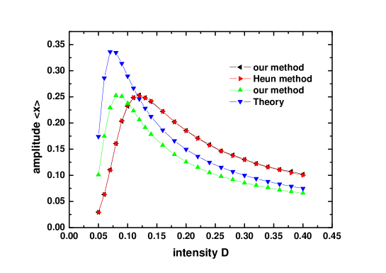
and the periodic driven force’s amplitude A and frequency ω𝜔\omega are 0.03 and 0.01 respectively. We consider the relation between the amplitude of output of the system <x>expectation𝑥<x> and the noise intensity D. The average is taken over 5×1055superscript1055\times 10^{5} realizations and the Heun method is used as a comparison. We then compare our results with the model mentioned in [23]:

x˙=V(x)+Acos(ωt)+ξ(t),<ξ(t)ξ(t)>=2Dδ(tt).formulae-sequence˙𝑥superscript𝑉𝑥𝐴𝜔𝑡𝜉𝑡expectation𝜉𝑡𝜉superscript𝑡2𝐷𝛿𝑡superscript𝑡\begin{split}&\dot{x}=-V^{{}^{\prime}}(x)+A\cos(\omega t)+\xi(t),\\ &<\xi(t)\xi(t^{{}^{\prime}})>=2D\delta(t-t^{{}^{\prime}}).\\ \end{split} (41)

The theoretical result of <x>expectation𝑥<x> in this model is <x>=AD2rk4rk2+ω2expectation𝑥𝐴𝐷2subscript𝑟𝑘4superscriptsubscript𝑟𝑘2superscript𝜔2<x>=\frac{A}{D}\frac{2r_{k}}{\sqrt{4r_{k}^{2}+\omega^{2}}}, where rk=12πexp(ΔVD)subscript𝑟𝑘12𝜋Δ𝑉𝐷r_{k}=\frac{1}{\sqrt{2}\pi}\exp{(-\frac{\Delta V}{D})}.

Refer to caption

Figure 4: Comparison of different numerical methods for the stochastic resonance in the noise-driven bistable system. The periodic driven force’s amplitude A and frequency ω𝜔\omega are 0.03 and 0.01, respectively. The friction coefficient γ𝛾\gamma is equal to 1. The amplitude of output is averaged over 5×1055superscript1055\times 10^{5} trajectories. The black line is our method with step size 0.1 and the red line is the Heun method with step size 0.01. Both the two lines have the characteristic time 1. The green line is our method with step size 0.1 and characteristic time 0.1. The blue line is the theoretical result of Eq.(41).

Fig.(4) shows the results of our simulations. The black line and the red line are the simulations of our method with step size 0.1 and the Heun method with step size 0.01 respectively, with the parameters γ𝛾\gamma and λ𝜆\lambda equal to 1. We now see that the results of our method and the Heun method are almost the same, however, the step size of our method is larger than the one used in Heun method. The parameters of the green line is the same as the black line except λ=10𝜆10\lambda=10, that is, the characteristic time is shorter, and in this condition, the Ornstein-Uhlenbeck noise is closer to the Gaussian noise. We can find that the resonant noisy intensity (the maximum of the line) shifts left when we shorten the characteristic time. In other words, lengthening the characteristic time can enhance the noise resistance of the system. The blue line is the theoretical result of Eq.(41). Since the influence of the inertia term x¨¨𝑥\ddot{x}, we can see that the amplitude of output <x>expectation𝑥<x> of the theoretical result is greater than our numerical result as shown in the green line.

5 Conclusion

We have proposed the bicolour rooted tree method to do the stochastic Taylor expansion systematically. This method can be used to solve the stochastic differential equation numerically. In this paper, we focus on the Langevin equation which is widely used in modern science. A high order algorithm o(7,4.5) is derived in this paper. Comparing with other usual algorithms, our method is advantageous in computational efficiency and accuracy. We present our method in the two examples. In the first example of energy relaxation in the double well, we show our method gives the same results as presented in other papers, and the convergence is better than the other algorithms. In the second example, we propose an algorithm for the time-dependent Langevin equation with the Ornstein-Uhlenbeck noise, and the result of our algorithm is the same as the one obtained by Heun method. It shows our algorithm is suitable for the Langevin equation regardless of the time-dependence of the equation. However, the readers should note that we only provide the algorithm for Eq.(17) which satisfies the property (19) since this property can drastically reduce the complexity of Eq.(14). For the other type of SDEs that the property (19) can not be held, such as the Hodgkin-Huxley model in neuroscience [27], interested readers can design their own algorithms based on the Eq.(14). For the purpose of using our method in the more difficult situations, one can consider the case that the diffusion coefficients are variable. All in all, we have provided a systematic scheme for searching the high order algorithm for the SDE and find that it can reduce drastically when deal with the Langevin equation.

Acknowledgments

The authors thank Prof. Yong Zhang for useful discussions and Dr. Jigger Cheh, Shaoqiang Yu for helping with the preparation of the paper. We also thank the anonymous referees for their helpful advice. This research was partly supported by National Basic Research Program of China (973 program) (Contract No. 2007CB814800) and National Natural Science Foundation of China (Contract No. 10475067).

References

  • [1] A. Glück, H. Hüffel, Phys. Lett. B 659 (2008) 447.
  • [2] E.V. Sukhorukov, A.N. Jordan, Phys. Rev. Lett. 98 (2007) 136803.
  • [3] S. Chandrasekhar, Rev. Mod. Phys. 15 (1943) 1.
  • [4] D.T. Gillespie, J. Chem. Phys. 113 (2000) 297.
  • [5] A.L.S. Chua, C.A. Haselwandter, C. Baggio, D.D. Vvedensky, Phys. Rev. E 72 (2005) 051103.
  • [6] C. Forrey, M. Muthukumar, Biophys. J. 91 (2006) 25.
  • [7] A. Naji, J. Chem. Phys. 126 (2007) 235103.
  • [8] J.P. Bouchaud, R. Cont, Eur. Phys. J. B 6 (1998) 543.
  • [9] Y. Gong, B. Xu, X. Ma, Chem. Phys. Lett. 458 (2008) 351.
  • [10] B. Geislinger, R. Kawai, Phys. Rev. E 74 (2006) 011912.
  • [11] S. Wallin, K.B. Zeldovich, E.I. Shakhnovich, J. Mol. Biol. 368 (2007) 884.
  • [12] Y. Wang, Q. Li, Biophys. Chem. 136 (2008) 32.
  • [13] R. Filliger, P. Reimann, Phys. Rev. Lett. 99 (2007) 230602.
  • [14] J. Berges, D. Sexty, Nucl. Phys. B 799 (2008) 306.
  • [15] E. Hershkovitz, J. Chem. Phys. 108 (1998) 9253.
  • [16] K. Burrage, P.M. Burrage, Appl. Numer. Math. 22 (1996) 81.
  • [17] J.C. Butcher, The Numerical Analysis of Ordinary Differential Equations, Wiley, London, 1987.
  • [18] P.E. Kloeden, E. Platen, The Numerical Solution of Stochastic Differential Equations, Springer-Verlag, Berlin, 1992.
  • [19] Our research group has an integrator using the 7th order Runge-Kutta method, the readers can refer to these two papers for more details: J.R. Dormand, P.J. Prince, Celest. Mech. Dyn. Astr. 18 (1978) 223; A. Huta, V. Penjak, Appl. Math. 29 (1984) 411.
  • [20] A. Greiner, W. Strittmatter, J. Honerkamp, J. Stat. Phys. 51 (1988) 95.
  • [21] R. Benzi, S. Sutera, A. Vulpiani, J. Phys. A 14 (1981) L453; R. Benzi, G. Parisi, A. Sutera, A. Vulpiani, Tellus 34 (1982) 10.
  • [22] C. Nicolis, G. Nicolis, Tellus 33 (1981) 225.
  • [23] L. Gammaitoni, P. Hänggi, P. Jung, F. Marchesoni, Rev. Mod. Phys. 70 (1998) 223.
  • [24] L. Gammaitoni, P. Hänggi, P. Jung, F. Marchesoni, Eur. Phys. J. B 69 (2009) 1.
  • [25] Matjaž Perc, Phys. Rev. E 76 (2007) 066203.
  • [26] P. Hänggi, ChemPhysChem 3 (2002) 285.
  • [27] Mahmut Ozer, Matjaž Perc, Muhammet Uzuntarla, Phys. Lett. A 373 (2009) 964.
  • [28] Qingyun Wang, Matjaž Perc, Zhisheng Duan, Guanrong Chen, Chaos 19 (2009) 023112.
  • [29] A. Rivas, N.P. Oxtoby, S.F. Huelga, Eur. Phys. J. B 69 (2009) 51.