Evolution of Social-Attribute Networks:
Measurements, Modeling, and Implications using Google+

Abstract

Understanding social network structure and evolution has important implications for many aspects of network and system design including provisioning, bootstrapping trust and reputation systems via social networks, and defenses against Sybil attacks. Several recent results suggest that augmenting the social network structure with user attributes (e.g., location, employer, communities of interest) can provide a more fine-grained understanding of social networks. However, there have been few studies to provide a systematic understanding of these effects at scale.

We bridge this gap using a unique dataset collected as the Google+ social network grew over time since its release in late June 2011. We observe novel phenomena with respect to both standard social network metrics and new attribute-related metrics (that we define). We also observe interesting evolutionary patterns as Google+ went from a bootstrap phase to a steady invitation-only stage before a public release.

Based on our empirical observations, we develop a new generative model to jointly reproduce the social structure and the node attributes. Using theoretical analysis and empirical evaluations, we show that our model can accurately reproduce the social and attribute structure of real social networks. We also demonstrate that our model provides more accurate predictions for practical application contexts.

1 Introduction

Online social networks (e.g., Facebook, Google+, Twitter) have become increasingly important platforms for interacting with people, processing information and diffusing social influence. Thus understanding social-network structure and evolution has important implications for many aspects of network and system design including bootstrapping reputation via social networks (e.g., [39]), defenses against Sybil attacks (e.g., [14]), leveraging social networks for search [1], and recommender systems with social regularization [35].

Traditional social network studies have largely focused on understanding the topological structure of the social network, where each user can be viewed as a node and a specific relationship (e.g., friendship, co-authorship) is represented by a link between two nodes. More recently, there has been growing interest in augmenting this social network with user attributes, which we call as Social-Attribute Network (SAN). User attributes could be static (e.g., school, major, employer and city derived from user profiles), or dynamic (e.g., online interest and community groups). Recent studies have demonstrated the promise of social-attribute networks in applications such as link prediction [58, 17], attribute inference [17, 58], and community detection [62].

Despite the growing importance of such social-attribute networks in social network analysis applications, there have been few efforts at systematically measuring and modeling the evolution of social-attribute networks. Most prior work in the measurement and modeling space focuses primarily on the social structure [3, 4, 13, 26, 28, 33, 38]. Measuring social-attribute networks can simultaneously inform us the properties of social network structure, attribute structure, and how such attributes impact social network structure.

In this paper, we present a detailed study of the evolution of social-attribute networks using a unique large-scale dataset collected by crawling the Google+ social network struture and its user profiles. This dataset offers a unique opportunity for us as we were fortunate to observe the complete evolution of the social network and its growth to around 30 million users within a span of three months.

We observe novel patterns in the growth of the Google+ social-attribute network. First, we observe that the social reciprocity of Google+ is lower than many traditional social networks and is closer to that of Twitter. Second, in contrast to many prior networks, the social degree distributions in Google+ are best modeled by a lognormal distribution. Third, we observe that assortativity of Google+ social network is neutral while many other social networks own positive assortativities. Fourth, we also see that the distinct phases (initial launch, invite only, public release) in the timeline of Google+ naturally manifest themselves in the social and attribute structures. Fifth, for the generalized attribute metrics (that we define), while some attribute metrics mirror their social counterparts (e.g., diameter), several show distributions and trends that are significantly different (e.g., clustering coefficient, attribute degree). Finally, via the social-attribute network framework, we study the impact of user attributes on the social structure and observe that nodes sharing common attributes are likely to have higher social reciprocity and that some attributes have much stronger influence than others (e.g., Employer vs. City).

Based on our observations, we develop a new generative model for SANs. Our model includes two new components, i.e., attribute-augmented preferential attachment and attribute-augmented triangle-closing, which extend the classical preferential attachment [5, 27] and triangle-closing [29, 43, 53, 2], respectively. Using both theoretical analysis and empirical evaluation, we show that our model can reproduce SANs that accurately reflect the true ones with respect to various network metrics and real-world applications. Such a generative model has a lot of applications [30] such as network extrapolation and sampling, network visualization and compression, and network anonymization [44].

To summarize, the key contributions of this work are:

• We perform the first study of the evolution of social-attribute networks using Google+. We observe novel phenomena in standard social structure metrics and new attribute-related metrics (that we define) and how attributes impact the social structure.

• We develop a measurement-driven generative model for the social-attribute network that models the impact of user attributes into the network evolution.

• Using both theoretical analysis and empirical evaluation, we validate that our model can accurately reproduce real social-attribute networks.

2 Preliminaries and Dataset

In this section, we begin with some background on augmenting social network structure with attributes. Then, we describe how we collected the Google+ data and how we augment the Google+ social network with user attribute information. We also present some basic measurements describing the evolution of the Google+.

2.1 Social-Attribute Network (SAN)

In this section, we review the definition of Social-Attribute Network (SAN) [17] and introduce the basic notations used in the rest of this paper.

Given a directed social network $G$, in which nodes are users and edges represent friend relationships between users, and $M$ distinct binary attributes, which could be static (e.g., name of employer, name of school, major, etc.) or dynamic (e.g., interest groups), a SAN is an augmented network with $M$ additional nodes where each such node corresponds to a specific binary attribute. For each node $u$ in $G$ with attribute $a$, we create an undirected link between $u$ and $a$ in the SAN.

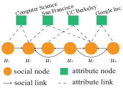
Figure 1: Illustration of a SAN with six social nodes and four attribute nodes. Note that the social links between users are directed whereas the attribute-user links are undirected.

Nodes in a SAN corresponding to nodes in $G$ are called social nodes and denoted as the set $V_{s}$, while nodes representing attributes are called attribute nodes and denoted as the set $V_{a}$. Figure 1 shows an example SAN. Links between social nodes are called social links and denoted as the set $E_{s}$, while links between social nodes and attribute nodes are called attribute links and denoted as the set $E_{a}$. Thus a Social-Attribute Network is denoted as $SAN=(V_{s},V_{a},E_{s},E_{a})$.

For a given social or attribute node $u$ in a SAN, we denote its attribute neighbors as $\Gamma_{a}(u)=\{v|v\in V_{a},(u,v)\in E_{a}\}$, social neighbors as $\Gamma_{s}(u)=\{v|v\in V_{s},(v,u)\in E_{s}\cup E_{a}\ or\ (u,v)\in E_{s}\cup E_{a}\}$, social in neighbors as $\Gamma_{s,in}(u)=\{v|(v,u)\in E_{s}\}$ and social out neighbors as $\Gamma_{s,out}(u)=\{v|(u,v)\in E_{s}\}$. Note that an attribute node can only have social neighbors.

2.2 Google+ Data

Google+ was launched with an invitation-only test phase on June 28, 2011, and opened to everyone 18 years of age or older on September 20, 2011. We believed this was a tremendous opportunity to observe the real-world evolution of a large-scale social-attribute network. Thus, we began to crawl daily snapshots of public Google+ social network structure and user profiles; our crawls lasted from July 6 to October 11, 2011. The first snapshot was crawled by breadth-first search (without early stopping). On subsequent days, we expanded the social structure from the previous snapshot. For most snapshots, our crawl finished within one day as Google did not limit the crawl rate during that time.

We believe our crawl collected a large Weakly Connected Component (WCC) of Google+. This may be surprising as many past attempts on Flickr, Facebook, YouTube etc., were unable to do so [38]. The key difference is that these were only able to access outgoing links. In contrast, each user in Google+ has both an outgoing list (i.e., “in your circles”) and an incoming list (i.e., “have you in circles”). This allows us to access both outgoing and incoming links making it feasible to crawl the entire WCC.

We have two points of reference that suggest our coverage is high ($\geq$ 70%): 1) TechCrunch estimated the number of Google+ users on July 12, 2011 is around 10 million [52]; our crawled snapshot on the same day has 7 million users. (2) Google announced 40 million users had joined Google+ in middle October [19]; our crawled snapshot on October 11 has around 30 million users.

We take each user $u$ in Google+ as a social node in SAN, and connect it to her outgoing friends via outgoing links and incoming friends via incoming links. We use four attribute types School, Major, Employer and City that were available and easy to extract. Specifically, we find all distinct schools, majors, employers and cities that appear in at least one user profile and use them as attribute nodes. Recall that a social node $u$ is connected to attribute node $a$ via an undirected link if $u$ has attribute $a$. In this way, we construct a SAN from each crawled snapshot, resulting in 79 SANs during the period from July 6 to October 11, 2011.

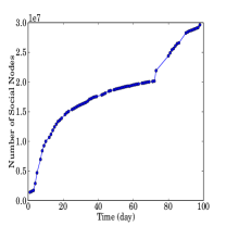
(a) Social nodes

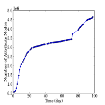
(b) Attribute nodes

Figure 2: Growth in the number of social and attribute nodes in the Google+ dataset.

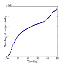
(a) Social links

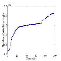
(b) Attribute links

Figure 3: Growth in the number of social and attribute links in the Google+ dataset

Figures 2 and 3 show the temporal evolution of the number of nodes and links in the Google+ SAN. From the results we clearly see three distinct phases in the evolution of Google+: Phase I from day one to day 20, which corresponds to the early days of Google+ whose size increased dramatically; Phase II from day 21 to day 75, during which Google+ went into a stabilized increase phase; and Phase III from day 76 to day 98, when Google+ opened to public (i.e., without requiring an invitation), resulting in a dramatic growth again. We point this out because we observe a similar three-phase evolution pattern for almost all network metrics that we analyze in the subsequent sections.

In the following sections, we use the last or largest snapshot, unless we are interested in the time-varying behavior.

Potential biases:  We would like to acknowledge two possible biases. First, users may keep some of their friends or circles private. In this case, we can only see the publicly visible list. Thus we may not crawl the entire WCC and underestimate the node degrees. However, as discussed earlier, we obtain a very large connected component that covers more than 70% of known users which is sufficiently representative. Second, users may choose not to declare their attributes, in which case we may underestimate the impact of attributes on the social structure. However, we find that roughly 22% of users declare at least one attribute which represents a statistically large sample from which to draw conclusions. Furthermore, by validating the attribute-related results via further subsampling the attributes we have, we show that our attributes are representative of the entire attributes.

3 Social Structure of the
Google+ SAN

In this section, we begin by presenting several canonical network metrics commonly used for characterizing social networks such as the reciprocity, density, clustering coefficient, and degree distribution [38, 25, 28, 41]. These metrics are useful to expose the inherent structure of a social network in terms of the friend relationships and whether there are “community” structures beyond a one-hop friend relationship. It is particularly useful to revisit these metrics in the context of Google+ both because of its scale and because it enables a somewhat hybrid relationship model compared to other networks such as Facebook, Twitter, Flickr, and email networks. Furthermore, since we have a unique opportunity to observe the network as it grew, we also analyze how these properties changed as the Google+ SAN evolved.

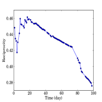
(a) Reciprocity

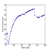
(b) Social density

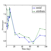
(c) Diameter

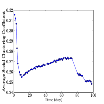
(d) Social clustering coefficient

Figure 4: Evolution of four key metrics: reciprocity, density, diameter and clustering coefficient on the Google+ SAN. In each case, we observe distinct behaviors in the three phases corresponding to early initialization, time to public release, and time after public release.

3.1 Reciprocity

The reciprocity metric for directed social networks represents the fraction of social links that are mutual; i.e., if there is a $A\rightarrow B$ edge what is the likelihood of the reverse $B\rightarrow A$ edge. Previous work studied the global reciprocities for specific snapshots of social networks and measured it to be $0.62$ on Flickr, $0.79$ on YouTube [38], and $0.22$ on Twitter [28]. We focus on the evolution of global reciprocity for Google+ in Figure 4a. The result shows an interesting behavior where the reciprocity fluctuates in Phase I, decreases in Phase II and decreases even faster in Phase III. We speculate that this arises because of the hybrid nature of Google+. Initially many people treat the network like a traditional social network (e.g., Facebook) where the relationships are mutual. However, as time progresses and people appear to become familiar with the Twitter-like publisher-subscriber model also offered by Google+, the reciprocity decreases.

3.2 Density

The ratio of links-to-nodes, $\frac{|E_{s}|}{|V_{s}|}$, captures the density of a social network. To put this in context, previous studies show that the social density increases over time on citation and affiliation networks [33], on Facebook [4], and fluctuates in an increase-decrease-increase fashion on Flickr [26], and is relatively constant on email communication networks [25].

Figure 4b shows the evolution of this social density metric in Google+. We observe that social density in Google+ network has a sharp decrease followed by an increase in Phase I, a continued increase in Phase II, and a sudden drop in Phase III (when Google+ opened to the public) followed by a steady increase again. This three-phase pattern can be explained in conjunction with the trends in Figures 2a and 3a. In the early part of Phase I, even though the rate of users joining Google+ is high, the rate of adding links is low, possibly because many of a user’s existing friends have not yet joined. This causes social density to decrease. As users acquire friends with a rate higher than the rate of new users in later part of Phase I and the same trend continuing in Phase II, the social density increases. In Phase III, the number of users in Google+ had a sudden jump due to the public release but the number friendship links increases less dramatically, which once again causes the social density to drop significantly around t=70, but then starts slowly increasing again. Our findings have implications for network modeling. Specifically, many network models either assume constant density [5, 24] or power-law densification [33], which is not consistent with Google+.

3.3 Diameter

In directed social networks, the distance between two user nodes $u$ and $v$, $dist(u,v)$ is defined as the length of the shortest directed path whose head is $v$ and tail is $u$. Note that only social links $E_{s}$ are used in this definition. We find that the distribution of the distance between nodes has a dominant mode at a distance of six, with most nodes (90%) having a distance of 5, 6, or 7 (not shown).

Based on the distance distribution, we can also define the effective diameter as the 90-th percentile distance (possibly with some interpolation) between every pair of connected nodes [33]. Unfortunately, computing the effective diameter is infeasible for large networks, so we use the HyperANF approximation algorithm [8], which has been shown to be able to approximate diameter with high accuracy.

Previous work observed effective diameter shrinks in citation networks, autonomous networks and affiliation network [33], in Flickr and Yahoo! 360 [26], and in Cyworld [3]. However, we observe that the effective diameter follows a three-phase evolution as seen in Figure 4c, which again can be explained in conjunction with the trends in Figures 2a and 3a. In Phase I, user joining rate outpaces link creation rate, causing the diameter to increase; in Phase II, user joining rate is lower than link acquisition rate, resulting in decreasing diameter; and in Phase III user joining rate is much higher, resulting in a diameter increasing phase again. Again, our observations have implications for network modeling. Existing network models either assume logarithmically growing diameter [55, 5] or shrinking diameter [30, 33].

3.4 Clustering Coefficient

Given a network $G$ and node $u$, $u$’s clustering coefficient is defined as

$$c(u)=\frac{L(u)}{|\Gamma_{s}(u)|(|\Gamma_{s}(u)|-1)},$$

where $L(u)$ is the number of links among $u$’s social neighbors $\Gamma_{s}(u)$ and the average social clustering coefficient is defined as $C_{s}=\frac{1}{|V_{s}|}\sum_{u\in V_{s}}c(u)$ [55]. Intuitively, this captures the community structure among a user’s friends.

Again, computing the average clustering coefficient is expensive. Thus, we extend the constant-time approximate algorithm proposed by Schank et al. for undirected networks [45], and develop an algorithm to approximate the clustering coefficients for a directed network. With $\lceil\frac{\mathrm{ln}2\nu}{2\epsilon^{2}}\rceil$ random samples, our constant time algorithms can bound the error of average clustering coefficient within $\epsilon$ with probability at least $1-\frac{1}{\nu}$. In practice, we set the error to be $\epsilon=0.002$ and $\nu=100$. Algorithm details and theoretical analysis can be found in Appendix A.

Kossinets et al. [25] observed constant average social clustering coefficient over time in an email communication network. However, we find that the evolution of average social clustering coefficient of Google+, which is shown in Figure 4d, again follows a three-phase evolution pattern where the clustering coefficient dramatically decreases in Phase I, increases slowly in Phase II and decreases again in Phase III. Our findings indicate that the community structure among users’ friends is highly dynamic, which inspires us to do dynamic community detection.

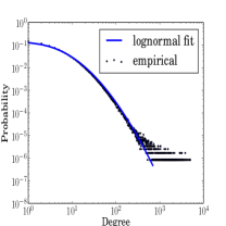
(a) Outdegree

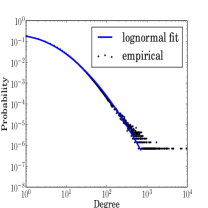
(b) Indegree

Figure 5: Indegree and outdegree distributions for the social nodes in the Google+ SAN along with their best-fit curves. We observe that both are best modeled by a discrete lognormal distribution unlike many networks that suggest power-law distributions.

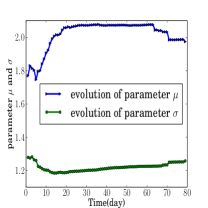
(a) Outdegree

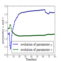
(b) Indegree

Figure 6: Evolution of the lognormal parameters for the indegree and outdegree distributions.

3.5 Degree Distributions

Next, we focus on the social indegree and outdegree of users in Google+. In each case, we are also interested in identifying an empirical best-fit distribution using the tool [54, 10], which compares fits of several widely used distributions (e.g., power-law, lognormal, power-law with cutoff using) with respect to goodness-of-fit. We find that unlike many studies on social networks, in which social degrees usually follow a power-law distribution [13, 38], social degrees are best captured by a discrete lognormal distribution in Google+. Recall that a random variable $x\in\mathbb{Z^{+}}$ follows a power-law distribution if $p(x=k)\propto k^{-\alpha}$, where $\alpha$ is the exponent of the power-law distribution. On the other hand, a random variable $x\in\mathbb{Z^{+}}$ follows a discrete lognormal distribution if $p(x=k)\propto\frac{1}{k}\text{exp}(-\frac{(\text{ln}k-\mu)^{2}}{2\sigma^{2}})$ [7], where $\mu$ and $\sigma$ are the mean and standard deviation respectively of the lognormal distribution.

Figure 5 shows these degree distributions and their discrete lognormal fits, and Figure 6 shows the evolutions of the parameters for the fitted discrete lognormal distributions. We see the evolution of the outdegree and indegree distributions follows a similar trend but with the fluctuation differing in magnitude (Figures 6a, 6b).

Lognormally distributed degree distributions imply that there are probabilistically more low degree social nodes in Google+ than those in power-law distributed networks.

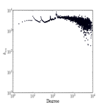
(a) $k_{nn}$ metric

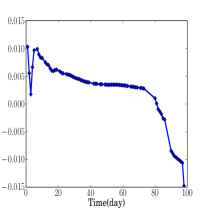
(b) Assortativity

Figure 7: Two metrics for capturing the joint-degree distribution: (a) $k_{nn}$ shows a log-log plot of the outdegree versus the average indegree of friends and (b) shows the evolution of the assortativity coefficient.

3.6 Joint Degree Distribution

Last, we examine the joint degree distribution (JDD) of the Google+ social structure. JDD is useful for understanding the preference of a node to attach itself to nodes that are similar to itself. One way to approximate the JDD is using the degree correlation function $k_{nn}$, which maps outdegree to the average indegree of all nodes connected to nodes of that outdegree [42, 38]. An increasing $k_{nn}$ trend indicates high-degree nodes tend to connect to other high-degree nodes; a decreasing $k_{nn}$ represents the opposite trend. Figure 7a shows the $k_{nn}$ function for Google+ social structure.

The JDD can further be quantified using the assortativity coefficient $r$ that can range from -1 to 1 [41]. $r$ is positive if $k_{nn}$ is positively correlated to node degree $k$. Figure 7b illustrates the evolution of the assortativity coefficient. We observe that $r$ keeps decreasing in all three phases but at different rates. Furthermore, unlike many traditional social networks where the assortativity coefficient is typically positive—0.202 for Flickr, 0.179 for LiveJournal and 0.072 for Orkut [38, 41]—Google+ has almost neutral assortativity close to 0. The neutral assortativity can possibly be explained by the hypothesis that Google+ is a hybrid of two ingredients, i.e., a traditional social network and a publisher-subscriber network (e.g., Twitter). Traditional social networks usually have positive assortativity; publisher-subscriber networks often have negative assortativity because high-degree publisher nodes tend to be connected to low-degree subscriber nodes. Thus a hybrid of them results in a network with neutral assortativity. The evolution pattern of Google+’ assortativity coefficient (i.e., positive in Phase I, around 0 in Phase II, and negative in Phase III) manifests the competing process of the two ingredients of Google+. More specifically, the traditional network ingredient slightly wins in Phase I, resulting in a slightly positive assortativity coefficient. A draw between them in Phase II results in the neutral assortativity. In Phase III, the publisher-subscriber ingredient wins, resulting in a slightly negative assortativity coefficient. This implies that Google+ is more and more like a publisher-subscriber network.

3.7 Summary of Key Observations and Implications

Analyzing the social structure of Google+ and its evolution over time, we find that:

• In contrast to many traditional networks, we find that Google+ has low reciprocity, the social degree distribution is best modeled by a lognormal distribution rather than a power-law distribution, and the assortativity is neutral rather than positive.

• Google+ is somewhere between a traditional social network (e.g., Flickr) and a publisher-subscriber network (e.g., Twitter), reflecting the hybrid interaction model that it offers. Moreover, it’s more and more closer to a publisher-subscriber network.

• The evolutionary patterns of various network metrics in Google+ are different from those in many traditional networks or assumptions of various network models. These findings imply that existing models cannot explain the underlying growing mechanism of Google+, and we need to design new models for reproducing social networks similar to Google+.

4 Attribute Structure of the
Google+ SAN

In the previous section we looked at well-known social network metrics. In this section, we focus on analyzing the attribute structure of the Google+ SAN. To this end, we extend the metrics from the previous section to the attributes as well. Finally, we show the importance of using attributes in understanding the social structure by studying their impact on metrics we analyzed earlier (e.g., reciprocity, clustering coefficient, and degree distribution). These attribute-related studies will characterize the attribute structure, give us insights about the underlying growing mechanism of Google+, and eventually guide us design a new generative model for Google+ SAN.

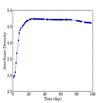
(a) Attribute density

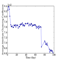
(b) Clustering coefficient

Figure 8: Evolution of the attribute density and average attribute clustering coefficient in the Google+ SAN.

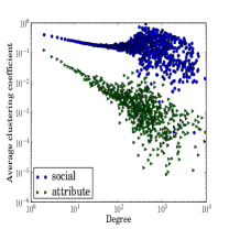
(a) Distributions in the original SAN

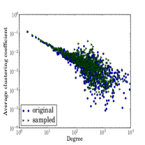
(b) Comparison with a subsampled SAN

Figure 9: Distributions of clustering coefficient with respect to node degrees. (a) Comparison of social and attribute clustering coefficient distributions in the original SAN. (b)Comparison of distributions of attribute clustering coefficients in the original SAN and the subsampled SAN.

4.1 Attribute Metrics

Density:  We consider a natural extension of the social density metric from

5 LABEL:

sec:socialdensity and define attribute density as $\frac{|E_{a}|}{|V_{a}|}$. Different from our observations with social density in Figure 4b, in Figure 8a, We observe the attribute density increases rapidly in Phase I, stays relatively flat in Phase II, and slightly decreases in Phase III. The reason for the decrease in Phase III is the large volume of new (i.e., non-invitation) users joining Google+ with many new attribute nodes whose social degrees are small.

Diameter:  We extend the distance metric from

6 LABEL:

sec:structure:distance to define the attribute distance between two attribute nodes $a$ and $b$ as $dist(a,b)=\text{min}\{dist(u,v)|u\in\Gamma_{s}(a),v\in\Gamma_{s}(b)\}+1$. Intuitively, attribute distance is the minimum number of social nodes that a attribute node has to traverse before reaching to the other one; i.e., attribute distance is the distance between two attribute communities. Similarly, we can consider the effective diameter using this attribute distance. Figure 4c also shows the evolution of the attribute diameter and shows that it very closely mirrors the social diameter.

Clustering coefficient:  Similarly, we generalize the social clustering coefficient from

7 LABEL:

sec:socialclustering to define the attribute clustering coefficient $c(u)$ for the attribute node $u$, and the average attribute clustering coefficient as $C_{a}=\frac{1}{|V_{a}|}\sum_{u\in V_{a}}c(u)$. This attribute clustering coefficient $c(u)$ characterizes the power of attribute $u$ to form communities among users who have the attribute $u$. Compared to Figure 4d, we find in Figure 8b that the average attribute clustering coefficient evolves in a different pattern since it’s relatively stable in Phase II.

We also show the distribution of average social and attribute clustering coefficients as a function of node degree in Figure 9a. We observe that both social and attribute clustering coefficients follow a power-law distribution with respect to node degrees, but attribute clustering coefficient distribution has a larger exponent. Moreover, we see that in general attribute clustering coefficients are lower because many shared attributes (e.g., city or major) will not naturally translate into a social relationship.

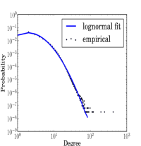
(a) Attribute degree of social nodes

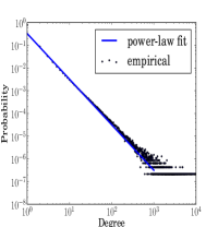
(b) Social degree of attribute nodes

Figure 10: Distributions of attribute-induced degrees in the Google+ SAN along with their best fits. The attribute degree of social nodes is best modeled by a lognormal whereas the social degree of attribute nodes is best modeled by a power-law distribution.

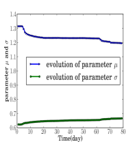
(a) Attribute degree of social nodes

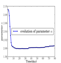
(b) Social degree of attribute nodes

Figure 11: Evolution in lognormal and power-law parameters for the attribute and social degree distributions

Degree distributions:  As discussed earlier, SANs introduce edges between social and attribute nodes. Thus, we consider two new notions of node degrees: (1) social degree of attribute nodes (i.e., the number of users that have this attribute) and (2) attribute degree of social nodes (i.e., the number of attributes each user has). We find that the attribute degree of social nodes is best modeled by a lognormal distribution whereas the social degree of attribute nodes is best modeled by a power-law distribution. Figure 10 and Figure 11 show the degree distributions and evolution of their fitted parameters.

In terms of the evolution, we find the attribute degree evolution seen in Figure 11 is significantly different from the previous observation in Figure 6: its mean decreases in Phase I, remains roughly constant in Phase II, and decreases again in Phase III. However, its standard deviation increases slightly in all phases. Finally, for the social degree which follows a power-law distribution, the exponent decreases fast in Phase I, and increases slightly in Phase II and Phase III.

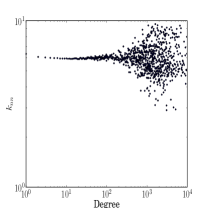
(a) Attribute $k_{nn}$

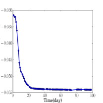
(b) Evolution of assortativity

Figure 12: (a) Joint degree of attribute nodes: Log-log plot of the social degree versus the average attribute degree of social neighbors of attribute nodes. (b) The evolution of the attribute assortativity coefficient.

Joint degree distribution:  Next, we extend the joint degree distribution (JDD) analysis to attribute nodes. For each social degree $k$, we compute $k_{nn}$ as the average attribute degree of social neighbors of attribute nodes that have social degree $k$. Intuitively, it captures the tendency of attribute nodes with high social degree to connect to social nodes with high attribute degree; i.e., if many nodes share a particular attribute, then are these nodes likely have many attributes? Figure 12 shows the $k_{nn}$ function for attribute JDD and the evolution of the attribute assortativity. Intuitively, we expect this relationship to be neutral and the result confirms this intuition; e.g., there are many Google+ users in New York but that does not imply the people in New York have many attributes. One interesting observation is that attribute assortativity coefficient evolves slightly differently compared to social assortativity coefficient (Figure 7b); it is stable in Phase III whereas social assortativity decreases significantly.

7.1 Influence on Social Network Structure

Next, we look at how attributes influence the social structure of the Google+ SAN w.r.t the metrics discussed in

8 LABEL:

sec:structure.

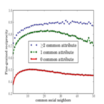
(a) Reciprocity

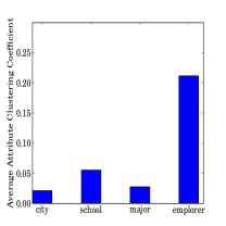
(b) Clustering coefficients

Figure 13: Influence of attribute on reciprocity and clustering coefficients.

Reciprocity:  We study how the number of common attribute neighbors influences reciprocity in conjunction with the number of common social neighbors. Let $a$ and $s$ denote the number of attribute and social neighbors of a given node, respectively. For each pair $(s,a)$, we compute $r_{s,a}$ as the percentage of links that are reciprocal among all the links whose endpoints have $s$ social neighbors and $a$ attribute neighbors.

To compute this, we look at all one directional links at the snapshot collected halfway and then compute the number of such links that become bidirectional at the last snapshot. We split these by the number of common social and attribute neighbors between these nodes at the halfway stage and show the $r_{s,a}$ values in Figure 13. We see that the reciprocity is almost twice as high for nodes that share common attribute neighbors compared to nodes without common attributes, regardless of the number of common social neighbors. While sharing common social neighbors improves link reciprocity, there is a natural diminishing returns property beyond 10 common social neighbors, and even decreasing for much larger values. We speculate that nodes sharing too many social neighbors are likely users with many “weak” ties. For recent reciprocity prediction problem [9, 21], our findings imply that any reciprocity predictor should incorporate node attributes instead of pure social structure metrics.

Clustering coefficient:  Next, we compute the average attribute clustering coefficient for the 4 attribute types: Employer, School, Major and City. For example, we compute the attribute clustering coefficients for all attribute nodes belonging to the attribute type Employer, and then average them to obtain the average attribute clustering coefficient for Employer. Figure 13b shows that attribute types vary in their influence on forming communities and that users with the same Employer attributes are much more likely to form communities than users sharing other attribute types. This has interesting implications for link prediction and attribute inference.

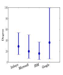
(a) Employer

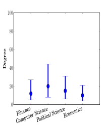
(b) Major

Figure 14: Influence of attribute on social degree

Degree distribution:  For brevity, we only focus on the Employer and Major attributes and show the result for the top attribute values observed within each category. We plot the median, 25^th, and 75^th percentile of the social outdegree of nodes that have these attribute values in Figure 14. We see that the users with Employer=Google and Major=Computer Science are likely to have higher degrees. We also computed the full degree distributions for these attribute values and saw that they follow different lognormal distributions (not shown). We speculate this could be a specific artifact of the Google+ network as many of the early adopters likely consist of Google employees and users in the IT/CS industry.

8.1 Validation via Subsampling

One natural question is whether the attributes of 22% of users we collected is a good representative of the entire attributes. To this end, we use subsampling method to validate our attribute-related results. We use attribute clustering coefficient distribution with respect to node degrees as an example, and observe similar results for other metrics. For each user with attributes, we remove her attributes with probability 0.5, from which we obtain a subsampled SAN. Then we calculate the attribute clustering coefficient distributions for the original and this subsampled SANs. Figure 9b shows that the results of the original and subsampled SANs are almost identical. Given the assumption that whether a user fills in her attributes is a random and independent event, our results demonstrate that the attributes of 22% of users is a representative sample of the attributes of all the users.

8.2 Summary of Key Observations and Implications

In this section, we studied the attribute structure of the Google+ SAN and how such attribute structure impacts the social structure. Our key observations are:

• While some attribute metrics mirror their social counterparts (e.g., diameter), several show distributions and trends that are significantly different (e.g., clustering coefficient, attribute degree). These observations will guide us to design models for SAN.

• We confirm that attributes have interesting impact on the social structure. e.g., nodes are likely to have higher reciprocity if they share common attributes. These findings have various implications. For instance, reciprocity predictor should incorporate node attributes.

• We also observe that some attribute types naturally have stronger influence than others. For example, users sharing the same employer have higher probability to be linked compared to users sharing the same city. Data mining tasks such as link prediction and attribute inference should potentially benefit from these findings.

9 A Generative Model For SAN

From the previous sections, we have seen novel phenomena in the social and attribute structure of the Google+ SAN and that the attribute structure impacts the social structure significantly. A natural question is whether we can create an accurate generative network model that can reproduce both the social and attribute structures we observe. Such a generative model can help us understand the growing mechanism of SAN, and allow other applications such as network extrapolation and sampling, network visualization and compression, and network anonymization [30].

Prior work on generative models focus primarily on the social structure [5, 24, 2, 33, 29]. Consequently, these approaches cannot model the attribute structure or their impact on social structure. To address this gap, we provide a new generative model taking into account the attribute structure from first principles rather than overlaying it after-the-fact. To this end, we extend a prior generative model [29], using attribute-augmented models for link generation and addition , which are key building blocks for such generative models. As we will show, this provides more realistic synthetic SAN that closely matches the Google+ SAN.

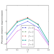
(a) PAPA model

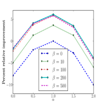
(b) LAPA model

Figure 15: Comparison between Power Attribute Preferential Attachment (PAPA) and Linear Attribute Preferential Attachment (LAPA) models. All result numbers are percentage of relative improvements over the loglikelihood of the PA model, i.e., with $\alpha$ =1 and $\beta$ = 0.

9.1 Building Block 1:
Attribute-Augmented Preferential Attachment

Leskovec et al. showed that the Preferential Attachment (PA) [5] is a suitable choice for creating edges [29]. The key idea in PA is that a new node $u$ is likely to connect to an existing node $v$ with a probability proportional to $v$’s degree. As we saw earlier, users who share attributes are also more likely to be connected. Thus, we consider two ways to augment the PA model:

• Power Attribute Preferential Attachment (PAPA):
  $f(u,v)$ $\propto$ $d_{i}(v)^{\alpha}(1+a(u,v)^{\beta})$

• Linear Attribute Preferential Attachment (LAPA):
  $f(u,v)$ $\propto$ $d_{i}(v)^{\alpha}(1+\beta\cdot a(u,v))$

Here, $f(u,v)$ is the probability with which social node $u$ adds a link to social node $v$, $d_{i}(v)$ is the indegree of $v$ and $a(u,v)$ is the number of common attributes that social nodes $u$ and $v$ share. Notice that when $\alpha$ = $\beta$ = 0, both reduce to a uniform distribution (i.e., $v$ is sampled uniformly at random) and when $\alpha$=1,$\beta$=0 both reduce to the PA model.

The relative improvement of a model with parameter $\alpha,\beta$ over the PA model is defined as $\frac{l_{PA}-l(\alpha,\beta)}{l_{PA}}$, where $l$ denote the log-likelihood of the model with respect to the empirically observed Google+ SAN. Figure 15 shows the relative improvements of these models over the PA model for varying values of $\alpha,\beta$. First, LAPA models perform better than PAPA models, which indicates that attribute likely influence friend requests in a linear way. Second, the PA model ($\alpha$ =1, $\beta$ = 0) is 7.9% better than a uniform random model ($\alpha$ =0, $\beta$ = 0). A LAPA model with $\alpha$ =1 and $\beta$ = 200 achieves a further 6.1% improvement over the PA model. Third, $\alpha=1$ achieves the best loglikelihood for any given $\beta$, which indicates that social degree has a linear effect on friend requests. In summary, we conclude that there is a combined linear effect of both social degree and attributes.

9.2 Building Block 2:
Attribute-Augmented Triangle-Closings

Triangle closing, where a node $u$ selects a node $v$ from its 2-hop neighbors and adds an edge, is an essential part of many generative network models [29, 61, 33, 2, 43, 53]. We explore if node attributes can improve triangle closing.

In the context of SAN, we can consider two types of triangle-closing: one is closing a triangle with no attribute node involved (e.g., $u_{4}\rightarrow u_{2}$ in Figure 1), and the other is closing a triangle which includes an attribute node (e.g., $u_{1}\rightarrow u_{2}$ in Figure 1). Following prior work, we refer them as triadic and focal closure respectively [25]. In the friend requests we observe in Google+, 84% percent are triadic (common friend), 18% percent are focal (common attribute), and 15% percent are cases where the nodes share both common friends and common attributes (e.g., $u_{6}\rightarrow u_{5}$ in Figure 1).

This suggests the importance of incorporating attributes in the triangle closure. To this end, we consider three models:

• Baseline: Select a social neighbor $v$ within a 2-hop radius uniformly at random.

• Random-Random (RR): Select a social neighbor $w\in\Gamma_{s}(u)$ uniformly at random, and then select a social neighbor $v\in\Gamma_{s}(w)$ uniformly at random which is shown to have very good performance in previous work [29].

• Random-Random-SAN (RR-SAN): select a neighbor $w\in\Gamma_{s}(u)\cup\Gamma_{a}(u)$ uniformly at random, and then select a social neighbor $v\in\Gamma_{s}(w)$ uniformly at random.

We compare these models using friend requests that are triadic closures, focal closures, or both. Our experimental results confirm that RR model performs 14% better than the Baseline model [29], and our RR-SAN model performs 36% better than RR model. This confirms that attributes play a significant role in the triangle-closing phenomenon as well and has natural implications for applications such as link prediction and friend recommendation.

1 T, simulated time steps

2 Initialization.

3 for $1\leq t\leq T$ do

4       Social node arrival. Sample a set of new social nodes $V_{t,new}$.

5       for $v_{new}\in V_{t,new}$ do

6             Attribute degree sampling. Sample the number of attributes $n_{a}(v_{new})$ for $v_{new}$ from a lognormal distribution.

7             for $1\leq i\leq n_{a}(v_{new})$ do

8                   Attribute linking.

9                  

10            end

11            First outgoing linking.

12            lifetime sampling.

13             sleep time sampling.

14            

15      end Collect woken social nodes $V_{t,woken}$.

16       for $v_{woken}\in V_{t,woken}$ do

17             Outgoing linking.

18             sleep time sampling.

19            

20      end

end

Algorithm 1 Social-Attribute Network Model

9.3 Our Generative Model for SAN

Our stochastic process models several key aspects of SAN evolution: node joining, how nodes issue outgoing links and receive incoming links, and how they link to attribute nodes. The key differences from prior work [29] are the two building blocks we described earlier: Linear Attribute Preferential Attachment (LAPA) and Random-Random-SAN (RR-SAN) triangle-closing.

Here, nodes arrive at some pre-determined rate. On arrival, each node picks an initial set of attributes and social neighbors (using the LAPA model). After joining the network, each node subsequently “sleeps” for some time, wakes up, and adds new links based on the RR-SAN model. We describe the model formally in Algorithm 1 and discuss each step next. From the analysis below, we find that the key step for generating lognormal social outdegree distribution is to make the lifetime of nodes follow a truncated normal distribution.

• Initialization: The SAN is initialized with a few social and attribute nodes and links. We observed that the starting point has no detectable influence when the number of initialization nodes is small compared to the overall network. We currently use a complete social-attribute network with 5 social nodes and 5 attribute nodes.

• Social node arrival: Social nodes arrive as predicted by a node arrival function $N(t)$, which could be estimated from real social networks. In our simulations, we simply let $N(t)=1$ modeling each node arrival as a discrete time step.

• Attribute degree: Each node picks some number of attributes sampled from a lognormal distribution with mean $\mu_{a}$ and variance $\sigma_{a}^{2}$.

• Attribute linking: Each new social node $v_{\mathit{new}}$ with $n_{a}(v_{\mathit{new}})$ attributes, we connect it to $n_{a}(v_{\mathit{new}})$ attribute nodes with the stochastic process defined as follows: for each attribute, with probability $p$, a new attribute node $a$ is generated; otherwise an existing attribute node $a$ is chosen with probability proportional to its social degree.

• First outgoing links: Each new node issues an outgoing link to a social node according to the LAPA model.

Lifetime sampling: The lifetime $l$ of $v_{\mathit{new}}$ is sampled from a truncated normal distribution, i.e., $p(l)\propto\text{exp}(-\frac{(l-\mu_{l})^{2}}{2\sigma_{l}^{2}})$ for $l\geq 0$. (Prior models use an exponentially distributed lifetime value [29, 61].)

Sleep time sampling: Sleep time $s$ of any node $v$ with outdegree $d_{o}$ can be sampled from any distribution with mean $m_{s}/d_{o}$. Our model only depends on mean sleep time. The intuition of making mean sleep time reversely proportional to outdegree is that a node with larger outdegree has higher tendency to issue outgoing links. (Prior models assume a power-law with cutoff distributed lifetime value [29, 61].)

Outgoing linking. Each woken social node $v_{\mathit{woken}}$ issues a new outgoing link according to our RR-SAN triangle-closing model.

9.4 Theoretical Analysis

By design, the attribute degree distribution of social nodes follows a lognormal distribution. Next, we show via analysis that the outdegree of social nodes and the social degree of attribute nodes follow a lognormal and power-law distribution respectively. For brevity, we provide a high-level sketch of the proofs.

Let $\phi(x)$ and $Φ\Phi(x)$ denote the probability density function and cumulative density function of standard normal distribution. Let $\gamma_{l}=-\frac{\mu_{l}}{\sigma_{l}}$, $g(\gamma)=\frac{\phi(\gamma)}{1-\Phi(\gamma)}$ and $\delta(\gamma)=g(\gamma)(g(\gamma)-\gamma)$.

Theorem 1

If the sleep time is sampled from some distribution with mean $m_{s}/d_{o}$, then the social out degrees of SANs generated by our model follow a lognormal distribution with mean $(\mu_{l}+\sigma_{l}g(\gamma_{l}))/m_{s}$ and variance $\sigma_{l}^{2}(1-\delta(\gamma_{l}))/m_{s}^{2}$.

Proof 9.2.

For any social node $v$, assume its final outdegree is $D_{o}$, then we have

$$\sum_{d_{o}=1}^{D}s(d_{o})\leq l,$$

where $s(d_{o})$ is the random sleep time whose mean is $m_{s}/d_{o}$. Thus, with mean-field approximation, we obtain

$$m_{s}\sum_{d_{o}=1}^{D}\frac{1}{d_{o}}\leq l.$$

Moreover, according to Euler’s asymptotic analysis on harmonic series, we have

$$\sum_{d_{o}=1}^{D}\frac{1}{d_{o}}\approx\text{ln}D_{o}.$$

That is, $\text{ln}D_{o}\approx l/m_{s}$. Lifetime $l$ is also a normal distribution truncated for $l\geq 0$, thus having mean $\mu_{l}+\sigma_{l}g(\gamma_{l})$ and variance $\sigma_{l}^{2}(1-\delta(\gamma_{l}))$. Thus, $\text{ln}D_{o}$ follows a truncated normal distribution with mean $\mu_{o}=(\mu_{l}+\sigma_{l}g(\gamma_{l}))/m_{s}$ and variance $\sigma_{o}^{2}=\sigma_{l}^{2}(1-\delta(\gamma_{l}))/m_{s}^{2}$. So $D_{o}$ follows a lognormal distribution with mean $\mu_{o}$ and variance $\sigma_{o}^{2}$.

Next, we derive the distribution of social degree of attribute nodes using mean-field rate equations [6].

Theorem 9.3.

The social degrees of attribute nodes in the SANs generated by our model follow a power-law distribution with exponent $\frac{2-p}{1-p}$.

Proof 9.4.

Without loss of generality, we assume one attribute link joins the SAN at each discrete time step. Let $D_{i}$ denote the social degree of the attribute node $i$ that joins the network at time $t_{i}$. According to the stochastic process in our algorithm, we have

$$\frac{dD_{i}}{dt}=\frac{(1-p)D_{i}}{\sum_{i}D_{i}}=\frac{(1-p)D_{i}}{t+m_{0}}$$

,where $m_{0}$ is the initial number of attribute links. Solving this ordinary differential equation with initial condition $D_{i}=1$ at $t=t_{i}$ gives us

$$D_{i}=(\frac{t+m_{0}}{t_{i}+m_{0}})^{(1-p)}.$$

So the probability of $D_{i}<D$ is

$$Pr(D_{i}<D)=1-Pr(t_{i}+m_{0}\leq(t+m_{0})D^{-\frac{1}{1-p}}).$$

According to our model, $Pr(t_{i})$ has a uniform distribution over the set $\{1,2,\cdots,t\}$. Thus we obtain

$$Pr(D_{i}<D)=1-\frac{(t+m_{0})D^{-\frac{1}{1-p}}-m_{0}}{t}.$$

Then the distribution of $D_{i}$ can be calculated as

$$Pr(D)=\frac{dPr(D_{i}\leq D)}{dD}=\frac{t+m_{0}}{t(1-p)}D^{-\frac{2-p}{1-p}}.$$

As $t\rightarrow\infty$, we obtain $Pr(D)\propto D^{-\frac{2-p}{1-p}}$. So the social degrees of attribute nodes follow a power-law distribution with exponent $\frac{2-p}{1-p}$.

Mitzenmacher [40] did a comprehensive study on generative models (e.g., PA, multiplicative models, random monkey) for power-law and lognormal distributions. In this work, we have proposed two new generative models.

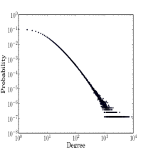
(a) Social outdegree

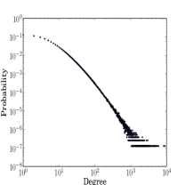
(b) Social indegree

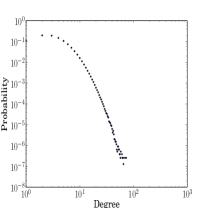
(c) Attribute degree of social nodes

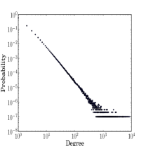
(d) Social degree of attribute nodes

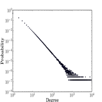
(e) Social outdegree

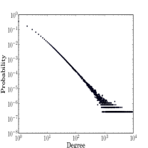
(f) Social indegree

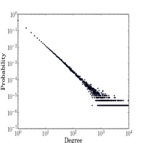
(g) Attribute degree of social nodes

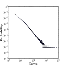
(h) Social degree of attribute nodes

Figure 16: Degree distributions of synthetically generated SAN using our model in (a)-(d) vs. Zhel shown in (e)-(h).

10 Evaluation

In this section, we validate our SAN generative model. Because the SAN area is still very nascent there are few standard models of comparison. We pick the closest generative model by Zheleva et al [61]. Note that their model is actually orthogonal to ours since it’s modeling dynamic node attributes while ours is modeling static node attributes. Furthermore, their original model generates undirected social networks. In order to compare with our model and directed Google+ SANs, we extend their model to generate directed social networks. We refer to the extended model as the Zhel model throughout this section. We start with network metrics, including single-node degree distribution, joint degree distribution and clustering coefficient. Then, following the spirit of [43], we also evaluate our model using real application contexts.

For comparison, we use the Google+ snapshot crawled on July 15, 2011, which has roughly 10 million nodes and we believe it is representative of Google+ SAN. Using this Google+ snapshot, we run a guided greedy search to estimate appropriate parameters for our model and Zhel to generate synthetic SAN that best match the Google+.

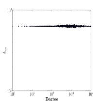
(a) JDD of attribute nodes

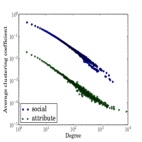
(b) Clustering coefficient

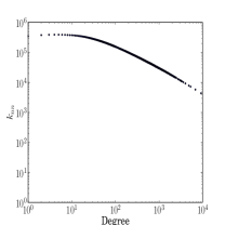
(c) JDD of attribute nodes

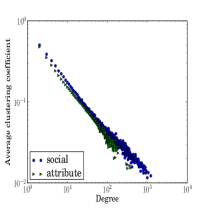
(d) Clustering coefficient

Figure 17: Joint degree and clustering coefficient distributions of our model (a)–(b) vs. Zhel in (c)–(d).

10.1 Network Metrics

In this section, we qualitatively compare our model to the Zhel model, and demonstrate that our model can generate synthetic SAN that better reproduces various network metrics closer to Google+ SAN.

Degree distributions:  We first examine the degree distributions of the synthetic SAN generated by our model and the Zhel model in Figure 16. The most visually evident result looking at Figure 16a and Figure 16b is that our model can generate synthetic networks with social indegree and outdegree following lognormal distributions similar to the Google+ SAN that we saw in Figure 5. In contrast, Figure 16f and Figure 16e confirm that the Zhel model generates indegree and outdegree following power-law distributions. Similarly, comparing Figure 16c and 16g to Figure 10a, the attribute degree of social nodes in our model follows the lognormal distribution that matches that of the Google+ SAN, whereas the Zhel model generates attribute degrees that follow a power-law distribution. Finally, Figure 16d and 16h confirm that both our model and Zhel generate social degrees of attribute nodes that follow power-law distribution, which is again consistent with Google+ SAN from Figure 10b.

Joint degree distributions:  The ability to mirror more fine-grained properties beyond the degree distributions has been shown to be a key metric for evaluating generative models [37]. Thus, we look at the joint degree distribution approximated by degree correlation function $k_{nn}$ in Figure 17a and 17c for our model and Zhel. Compared to Figure 12, we see that the JDD of attribute nodes in our model generated SAN matches Google+ SAN much better than Zhel. We observe similar pattern for JDD of social nodes.

Clustering coefficient:  Fig. 17b and Fig. 17d shows the clustering coefficient distributions of synthetic SANs generated by our model and Zhel, respectively. When comparing them to Fig. 9a we see that our model generates synthetic SAN with both social and attribute clustering coefficient distributions matching well to those of Google+ SAN, which is not the case for Zhel.

Significance of building blocks:  Recall that our model has two key building blocks that extend preferential attachment via LAPA and also extending triangle closing via focal closure. A natural question is what each of these components contribute toward the overall generative model.

First, we investigate how LAPA impacts the structure of the generated SAN in our model. To this end, we consider an intermediate model with the classical PA (but with the RR-SAN enabled) and compute the previous metrics for SANs generated by this intermediate model. We find that all metrics except the distribution of social indegree are qualitatively the same. Figure 18a shows that the distribution of social indegree of the synthetic SAN generated by our intermediate model is very close to a power-law distribution, different from the lognormal distribution generated by our full model shown in Figure 16b and derived from the real Google+ SAN shown in Figure 5. This suggests that the LAPA component is necessary for modeling a key aspect of the Google+ SAN.

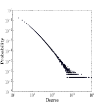
(a) Social indegree w/o LAPA

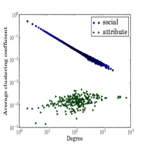
(b) Clustering coefficient w/o focal closure

Figure 18: The effect of LAPA and focal closure.

Second, we investigate the impact of RR-SAN. The key metric impacted by the focal closure component of RR-SAN is the attribute clustering coefficient. Figure 18b shows the social and attribute clustering coefficients of synthetic SANs generated by our model without RR-SAN (with classical RR enabled). Looking at Figure 17b and Figure 18b together, we see that RR-SAN has a significant impact on the attribute clustering coefficient.

These results confirm both attribute-augmented building blocks, LAPA and RR-SAN, play important but complementary roles in our model in generating synthetic SAN that closely mirrors the real Google+ SAN.

10.2 Application Fidelity

Next, we use two real-world application contexts to evaluate the fidelity of our generative model and the Zhel model with respect to a real Google+ snapshot. In each case, we use the metric of interest relevant to each application. Note that all these applications only rely on the social structure.

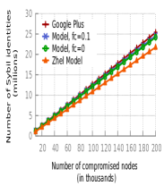
(a) Sybil defense

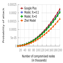
(b) Anonymous communication

Figure 19: Application fidelity of our model. (a) Sybil defense: SybilLimit false negatives as a function of number of compromised nodes. (b) Social network based anonymity: Probability of end-to-end timing analysis as a function of number of compromised nodes.

Sybil defense:  In a Sybil attack [14], a single entity emulates the behavior of a large number of identities to compromise the security and privacy properties of a system. Sybil attacks are of particular concern in decentralized systems, which lack mechanisms to vet identities and perform admission control. Several recent works have proposed the use of social trust relationships to mitigate Sybil attacks [14, 59]. Next, we show the fidelity of our model using a representative social network based Sybil defense mechanism called SybilLimit [59].

In order to prevent an adversary from obtaining a large number of attack edges (edges between compromised and honest users), SybilLimit bounds the effective node degree in the social network topology. Following their guidelines, we also imposed a node degree bound of 100 in evaluating their proposal on the different SANs. Figure 19a depicts the number of Sybil identities that an adversary can insert, as a function of number of compromised nodes in the network. We compromised the nodes uniformly at random, and set the SybilLimit parameter $w=10$. The parameter $fc$ governs the attribute link weight in our RR-SAN component; $fc=0$ means no focal closure.

We can see that (a) SybilLimit results using the synthetic topology generated by our model are a close match to the real Google+ data, and (b) our model outperforms the baseline approach (Zhel model). For example, when the number of compromised nodes is 200,000 the average number of Sybil identities in the Google+ topology is about 25.3 million, while our model predicts 24.5 million (error of 3.1% using $fc=0.1$). In contrast, the baseline approach has almost 4$\times$ worse error with a prediction error of 12.5%. This shows the importance of using attribute information to influence the structure of the social structure (the Zhel model only uses the social structure to influence the attribute structure.)

Anonymous communication:  Anonymous communication aims to hide user identity (IP address) from the recipient (destination) or from third parties on the Internet such as autonomous systems. The Tor network [12] is a deployed system for anonymous communication that serves hundreds of thousands of users a day. It is widely used by political dissidents, journalists, whistle-blowers, and even law enforcement/military. Recent work [22, 11] has proposed leveraging social links in building anonymous paths for improving resistance to attackers. For example, the Drac [11] system selects proxies (onion routers) by performing a random walk on the social network. For low-latency communications, if the first and the last hops of the forwarding path (onion routing circuit) are compromised, then the adversary can perform end-to-end timing analysis and break user anonymity. Figure 19b depicts the probability of end-to-end timing analysis when random walks on social networks are performed for anonymous communication, using the Google+ social network and our synthetic network. Similar to our SybilLimit experiments, we compromise nodes uniformly at random in the network, and impose an upper bound of 100 on the node degree. Again, we can see the accuracy of our model, as well as the improvement over prior work.

10.3 Summary

Via evaluating our model with respect to network metrics and real-world applications, we find that:

• Our model can reproduce SANs that well match Google+ SAN with respect to various network metrics (e.g., degree distributions, joint degree distributions and clustering coefficients.), but the Zhel model cannot match several metrics (e.g., social degree distributions, joint degree distributions and clustering coefficient.).

• Our model also performs better than the Zhel model for real-world applications such as Sybil defense and anonymous communication.

• The two attribute-augmented building blocks, i.e., LAPA and RR-SAN, play important but complementary roles in our model.

11 Discussion

Using attributes to strengthen defenses:  Our evaluation largely focuses on how our model better matches the real-world SAN. We hypothesize that several attack defenses (e.g., Sybil proofing) can also be enhanced by taking into account the attribute structure. For example, we could check if the attribute structure of the nodes matches normal nodes, or even if an attacker manages to obtain a “compromised” edge to one node we can limit the influence of this compromised edge by checking the attribute structure.

LAPA Computation:  The LAPA model as described requires a costly linear time (in number of nodes) step when a new node arrives. This is because we have to consider the number of common attributes between the new node and each current node, unlike PA which only needs the global degree distribution. Fortunately, we can approximate LAPA using a practical heuristic. The high-level idea is to pick one of the new node’s attributes at random and use PA within the nodes having this attribute. This approximates LAPA as nodes sharing more attributes are more likely to get selected.

Dynamic attributes:  Our model currently focuses on static attributes that nodes pick when they join the SAN. In our future work, we plan to incorporate dynamic attributes, and investigate whether the static attribute structure also influences the selection of dynamic attributes. Note that static attributes influence the social structure in our model while the dynamic attributes are influenced by the social structure in the model from Zheleva et al [61].

Parameter inference:  We currently use a guided greedy search to empirically estimate model parameters. While this works quite well, we plan to develop a more rigorous parameter inference algorithm based on maximum-likelihood principle [31, 57].

Parsimoniousness of our model:  In

12  

10, we have shown that each component of our model is necessary. However, it’s an interesting future work to design a more parsimonious model.

Implications for social network designs:  Our results that users sharing common employer attributes are more likely to be linked than users sharing other attributes can help design a better friend recommendation system, which is a very fundamental component of online social networks.

Relationship to heterogeneous networks:  Our SAN can be viewed as a heterogeneous network since it consists of multiple types of nodes and links. Heterogeneous networks are shown recently to work better than traditional homogeneous networks for various data mining tasks such as link prediction [17, 58, 48, 49], attribute inference [17, 58] and community detection [51, 50, 62]. It is an interesting future work to generalize our new attribute-related metrics and generative model to other heterogeneous networks.

13 Related Work

Given the growing role of social networks in users’ lives and the potential for using such insights for building better systems and applications, there is a rich literature on measuring and modeling social networks. Next, we discuss our work in the context of this related work. At a high-level, our specific new contributions are: (1) we characterize the evolution of a new large-scale network (Google+), and (2) we provide measurement-driven insights and models on the impact of attributes on social network evolution.

Measuring social networks:  Many prior efforts characterize social networks using the network metrics we also describe in

14 LABEL:

sec:structure [26, 28, 29, 38, 25]. Most of these focus on static snapshots; a few notable work also focus on evolutionary aspects similar to our work [3, 56, 4]. With multiple Google+ snapshots crawled around its public release, Schioberg et al. [46] studied a few network metrics, geographic distribution of the users and links, and correlation of users’ public information of Google+.

Concurrently, Gonzalez et al. [18] characterize several key features of Google+ during its first 10 months, and compare them to those of Facebook and Twitter. Using a static Google+ snapshot crawled after its public release, Magno et al. [36] identify the key differences between Google+ and Facebook and Twitter, study the adoption patterns of Google+ in different countries, and characterize the variation of privacy concerns across different cultures. Zhao et al. [60] study the early evolution of the Renren social network, and analyze its network dynamics at different granularities to determine their influence on individual users. While we follow the spirit of these works, our work is unique in terms of the specific dataset (i.e., three phases of Google+), the scale of the network, and the fact that we had a singular opportunity to study the evolution across different phases.

There has been recent realization of the importance of user attributes in characterizing social networks [38, 61]. These focus on the influence of social structure on dynamic node attributes (e.g., interest groups). Our work focuses on the orthogonal dimension of analyzing and modeling the influence of static node attributes on social structure formation using Google+.

Modeling social networks:  There are two broad classes of models for generating social networks: static and dynamic. Static models try to reproduce a single static network snapshot [15, 55, 37, 47]. Dynamic models can provide insights on how nodes arrive and create links; these include models such as preferential attachment [5], copying [24], nearest neighbor [2], forest fire [33]. Sala et al. [43] evaluated such models using both network metrics and application benchmarks and showed that the nearest neighbor model outperforms others. The dynamic/generative model by Leskovec et al. mimics the nearest neighbor model in a dynamic setting [29], and thus we use it as our starting point in

15 LABEL:

sec:model, However, these models are known to generate networks with power-law degree distributions. Many social networks including Google+, however, exhibit lognormal degree distributions [16, 32, 34]. Our dynamic model extends these prior work to provably generate a lognormal distribution for social outdegree. Our model also provides a more general framework by capturing both social and attribute structure.

Modeling social-attribute networks:  There has been relatively little work on generating SANs, though a few recent work jointly generating both social structure and node attributes can be viewed as SAN models; the most relevant work is from Zheleva et al. [61] and Kim and Leskovec [23]. Zheleva et al. [61] focus on dynamic attributes; their model generates undirected networks with power-law distribution for social degree and non-lognormal distribution for attribute degree (see Figure 16). Kim and Leskovec model the social and attribute structure simultaneously [23]. Here, both the social degree of attribute nodes and attribute degrees of social nodes follow binomial distribution, which differs from empirically observed SANs. Our model can generate SANs that we confirm through both analysis and simulations to be consistent with real SANs.

16 Conclusion

Using a unique dataset collected by crawling Google+ since its launch in June 2011, we provide a first-principled understanding of the attribute structure and its impact on the social structure and their evolutions with the SAN model. We observe several interesting phenomena in the structure and evolution of Google+. For example, the social degree distributions are lognormal, the assortativity is neural while many other social networks have positive assortativities, and the distinct phases in the evolution manifest themselves in the network structure. We also provide new metrics for characterizing the attribute structure and demonstrate that attributes can significantly impact the social structure. Building on these empirical insights, we provide a new generative model for SANs and validate that it is close to the real Google+ SAN using both network metrics and real application contexts. We believe that our work is one of the first steps in this regard and that there are several interesting directions for future work to harness the power of using the attribute structure for designing better social network based systems and applications.

17 Acknowledgments

We would like to thank Mario Frank, our shepherd Ben Zhao and the anonymous reviewers for their insightful feedback. This work is supported by the NSF TRUST under Grant No. CCF-0424422, NSF Detection under Grant no. 0842695, by the AFOSR under MURI Award No. FA9550-09-1-0539, by the Office of Naval Research under MURI Grant No. N000140911081, the NSF Graduate Research Fellowship under Grant No. DGE-0946797, the DoD National Defense Science and Engineering Graduate Fellowship, by Intel through the ISTC for Secure Computing, and by a grant from the Amazon Web Services in Education program. Any opinions, findings, and conclusions or recommendations expressed in this material are those of the author(s) and do not necessarily reflect the views of the funding agencies.

Input: $(SAN,\Omega,K)$, where $SAN=(V_{s},V_{a},E_{s},E_{a})$, $\Omega$ is the set of nodes whose average clustering coefficient $C_{\Omega}$ is approximated and $K$ is the number of samples needed.

Output: Approximate average clustering coefficient $\tilde{C}_{\Omega}$.

1 begin

2       $L\longleftarrow 0$

3       $k\longleftarrow 0$

4       while $k<K$ do

5             $k\longleftarrow k+1$

6             Sample a node $u$ uniformly at random from $\Omega$

7             Sample a pair of nodes $v$ and $w$ uniformly at random from $u^{\prime}s$ social neighbors $\Gamma_{s}(u)$

8             $L\longleftarrow L+F(v,u,w)$

9            

10      end $\tilde{C}_{\Omega}\longleftarrow L/(2^{I}K)$

11      

12end

Algorithm 2 Constant Time Approximate Algorithm for Computing the Average Clustering Coefficient

Appendix A A Constant Time Algorithm for Approximating Clustering Coefficients

Before going to details of the algorithm and analysis, we introduce a few notations. In both directed or undirected SANs, a triple $t$ consists of three nodes $(v,u,w)$ satisfying $v,w\in\Gamma_{s}(u)$, where $u$ is called the center and $v,w$ are called the endpoints of $t$. Moreover, $\alpha_{t}$ and $\beta_{t}$ denote respectively the center node and the two endpoints of $t$.

For a directed SAN and a set of triples $T$, we define a mapping $F:T\longrightarrow\{0,1,2\}$, where $F(t=(v,u,w))=0$ if $v$ and $w$ are not connected, $F(t=(v,u,w))=1$ if they are connected by one directed link and $F(t=(v,u,w))=2$ if they are reciprocally linked. For an undirected SAN, the mapping is defined as $F:T\longrightarrow\{0,1\}$, where $F(t=(v,u,w))=0$ if $v$ and $w$ are not connected, otherwise $F(t=(v,u,w))=1$. Let $I$ be an indicator variable of the directedness of a SAN, where $I=0$ when the SAN is undirected, otherwise $I=1$. With the indicator variable $I$, we have $0\leq F(t)\leq 2^{I}$, which is useful for deriving the approximation bounds in the follows.

For any set of nodes $\Omega$, their average clustering coefficient can be represented as $C_{\Omega}=\frac{1}{|\Omega|}\sum_{u\in\Omega}c(u)=2^{-I}\sum_{t\in T_{\Omega}}\frac{1}{|\Omega|\tau(\alpha_{t})}F(t)$, where $T_{\Omega}=\{t|\alpha_{t}\in\Omega\}$ and $\tau(\alpha_{t})=\frac{1}{2}|\Gamma_{s}(\alpha_{t})|(|\Gamma_{s}(\alpha_{t})|-1)$ is the number of triples whose center node is $\alpha_{t}$. If $t$ is a uniformly distributed random variable over $\Omega$, then we have $C_{\Omega}=2^{-I}E[F(t)]$. This observation informs us the design of our approximate algorithm, which is shown in Algorithm 2. Our algorithm computes the average social clustering coefficient when setting $\Omega=V_{s}$, and the average attribute clustering coefficient when setting $\Omega=V_{a}$. Note that our algorithm can also be used to compute average clustering coefficient distribution with respect to node degrees. The following theorem bounds the error of our algorithm.

Theorem A.5.

With the number of samples $K=\lceil\frac{\mathrm{ln}2\nu}{2\epsilon^{2}}\rceil$, the approximated average clustering coefficient $\tilde{C}_{\Omega}$ output by our algorithm satisfies $|\tilde{C}_{\Omega}-C_{\Omega}|\leq\epsilon$ with probability at least $1-\frac{1}{\nu}$.

Proof A.6.

Assume $t_{1},t_{2},\cdots,t_{K}$ are $K$ independently and uniformly distributed random variables over the triple set $T_{\Omega}$. Then we have $C_{\Omega}=E[\frac{1}{2^{I}K}\sum_{i=1}^{K}F(t_{i})]$. According to Hoeffding’s bound [20], we obtain

$$Pr(|\frac{1}{K}\sum_{i=1}^{K}F(t_{i})-E[\frac{1}{K}\sum_{i=1}^{K}F(t_{i})]|\geq 2^{I}\epsilon)\leq 2e^{-2K\epsilon^{2}}.$$

Thus,

$$Pr(|\tilde{C}_{\Omega}-C_{\Omega}|\leq\epsilon)\geq 1-2e^{-2K\epsilon^{2}}.$$

So we get $K=\lceil\frac{\mathrm{ln}2\nu}{2\epsilon^{2}}\rceil$ by setting $\nu=2e^{-2k\epsilon^{2}}$.

References

- [1] Microsoft Bing Social vs. Google Search Plus Your World: Showdown. http://www.pcworld.com/article/255476/microsoft_bing_social_vs_google_search_plus_your_world_showdown.html.
- [2] A. Vazquez. Growing network with local rules: Preferential attachment, clustering hierarchy, and degree correlations. Physical Review E (2003).
- [3] Ahn, Y.-Y., Han, S., Kwak, H., Moon, S., and Jeong, H. Analysis of topological characteristics of huge online social networking services. In WWW (2007).
- [4] Backstrom, L., Boldi, P., Rosa, M., Ugander, J., and Vigna, S. Four degrees of separation. In WebSci (2012).
- [5] Barabási, A.-L., and Albert, R. Emergence of scaling in random networks. Science 286 (1999), 509–512.
- [6] Barabási, A.-L., Albert, R., and Jeong, H. Mean-field theory for scale-free random networks. Physica A 272 (1999).
- [7] Bi, Z., Faloutsos, C., and Korn., F. The dgx distribution for mining massive, skewed data. In KDD (2001).
- [8] Boldi, P., Rosa, M., and Vigna, S. Hyperanf: Approximating the neighbourhood function of very large graphs on a budget. In WWW (2011).
- [9] Cheng, J., Romero, D., Meeder, B., and Kleinberg, J. Predicting reciprocity in social networks. In IEEE Conference on Social Computing (2011).
- [10] Clauset, A., Shalizi, C. R., and Newman, M. E. J. Power-law distributions in empirical data. SIAM Review, 51 (2009).
- [11] Danezis, G., Diaz, C., Troncoso, C., and Laurie, B. Drac: an architecture for anonymous low-volume communications. In PETS (2010).
- [12] Dingledine, R., Mathewson, N., and Syverson, P. Tor: The second-generation onion router. In USENIX Security (2004).
- [13] Dong, Z.-B., Song, G.-J., Xie, K.-Q., and Wang, J.-Y. An experimental study of large-scale mobile social network. In WWW (2009).
- [14] Douceur, J. R. The sybil attack. In Proc. IPTPS (2002).
- [15] Erdős, P., and Rényi., A. On random graphs i. Publ. Math. Debrecen 6 (1959), 290–297.
- [16] Gómez, V., Kaltenbrunner, A., and López, V. Statistical analysis of the social network and discussion threads in slashdot. In WWW (2008).
- [17] Gong, N. Z., Talwalkar, A., Mackey, L., Huang, L., Shin, E. C. R., Stefanov, E., Shi, E., and Song, D. Jointly predicting links and inferring attributes using a social-attribute network (san). In SNA-KDD (2012).
- [18] Gonzalez, R., Cuevas, R., Rejaie, R., and Cuevas, A. Google+ or google-?: Examining the popularity of the new OSN. In arXiv:1205.5662v2 (2012).
- [19] Google evidence of the high coverage of our crawled dataset. https://plus.google.com/106189723444098348646/posts/EanXz8fLwDh.
- [20] Hoeffding, W. Probability inequalities for sums of bounded random variables. Journal of the American Statistical Association 58, 301 (1963), 713–721.
- [21] Hopcroft, J., Lou, T., and Tang, J. Who will follow you back? reciprocal relationship prediction. In CIKM (2011).
- [22] Johnson, A., Syverson, P. F., Dingledine, R., and Mathewson, N. Trust-based anonymous communication: adversary models and routing algorithms. In ACM CCS (2011).
- [23] Kim, M., and Leskovec, J. Multiplicative attribute graph model of real-world networks. Internet Mathematics 8, 1-2 (2012), 113–160.
- [24] Kleinberg, J. M., Kumar, S. R., Raghavan, P., Rajagopalan, S., and Tomkins, A. The web as a graph: Measurements, models and methods. In Proceedings of the International Conference on Combinatorics and Computing (1999).
- [25] Kossinets, G., and Watts, D. Empirical analysis of an evolving social network. Science (2006).
- [26] Kumar, R., Novak, J., and Tomkins, A. Structure and evolution of online social networks. In KDD (2006).
- [27] Kumar, R., Raghavan, P., Rajagopalan, S., Sivakumar, D., Tomkins, A., and Upfal, E. Stochastic models for the web graph. In FOCS (2000).
- [28] Kwak, H., Lee, C., Park, H., and Moon, S. What is twitter, a social network or a news media? In WWW (2010).
- [29] Leskovec, J., Backstrom, L., Kumar, R., , and Tomkins, A. Microscopic evolution of social networks. In KDD (2008), pp. 462–470.
- [30] Leskovec, J., Chakrabarti, D., Kleinberg, J., Faloutsos, C., and Ghahramani, Z. Kronecker graphs: An approach to modeling networks. Journal of Machine Learning Research (JMLR) (2010).
- [31] Leskovec, J., and Faloutsos, C. Scalable modeling of real graphs using kronecker multiplication. In Proceedings of ICML (2007), pp. 497–504.
- [32] Leskovec, J., and Horvitz, E. Planetary-scale views on a large instant-messaging network. In WWW (2008).
- [33] Leskovec, J., Kleinberg, J. M., and Faloutsos, C. Graphs over time: densification laws, shrinking diameters and possible explanations. In KDD (2005), pp. 177–187.
- [34] Liben-Nowell, D., Novak, J., Kumar, R., Raghavan, P., and Tomkins, A. Geographic routing in social networks. PNAS 102, 33 (2005).
- [35] Ma, H., Zhou, D., Liu, C., Lyu, M. R., and King, I. Recommender systems with social regularization. In WSDM (2011).
- [36] Magno, G., Comarela, G., Saez-Trumper, D., Cha, M., and Almeida, V. New kid on the block: Exploring the google+ social graph. In IMC (2012).
- [37] Mahadevan, P., Krioukov, D., Fall, K., and Vahdat, A. Systematic topology analysis and generation using degree correlations. In SIGCOMM (2006).
- [38] Mislove, A., Marcon, M., Gummadi, K. P., Druschel, P., and Bhattacharjee, B. Measurement and analysis of online social networks. In Proc. of ACM SIGCOMM Internet Measurement Conference (2007).
- [39] Mislove, A., Post, A., Gummadi, K. P., and Druschel, P. Ostra: Leveraging trust to thwart unwanted communication. In Proc. NSDI (2008).
- [40] Mitzenmacher, M. A brief history of generative models for power law and lognormal distributions. Internet Mathematics 1, 2 (2003), 226–252.
- [41] Newman, M. E. J., and Park, J. Why social networks are different from other types of networks. Phys. Rev. E 68, 3 (2003).
- [42] Pastor-Satorras, R., Vazquez, A., and Vespignani, A. Dynamical and correlation properties of the Internet. Phys. Rev. Lett. 87 (2001).
- [43] Sala, A., Cao, L., Wilson, C., Zablit, R., Zheng, H., and Zhao, B. Y. Measurement-calibrated graph models for social network experiments. In WWW (2010).
- [44] Sala, A., Zhao, X., Wilson, C., Zheng, H., and Zhao, B. Y. Sharing graphs using differentially private graph models. In IMC (2011).
- [45] Schank, T., and Wagner, D. Approximating clustering coefficient and transitivity. Journal of Graph Algorithms and Applications 9, 2 (2005), 265–275.
- [46] Schioberg, D., Schneider, F., Schioberg, H., Schmid, S., Uhlig, S., and Feldmann, A. Tracing the birth of an osn: Social graph and profile analysis in google+. In WebSci (2012).
- [47] Stanton, I., and Pinar, A. Constructing and sampling graphs with a prescribed joint degree distribution. CoRR abs/1103.4875 (2012).
- [48] Sun, Y., Barber, R., Gupta, M., Aggarwal, C. C., and Han, J. Co-author relationship prediction in heterogeneous bibliographic networks. In ASONAM (2011).
- [49] Sun, Y., Han, J., Aggarwal, C. C., and Chawla, N. V. When will it happen?: relationship prediction in heterogeneous information networks. In WSDM (2012).
- [50] Sun, Y., Norick, B., Han, J., Yan, X., Yu, P. S., and Yu, X. Integrating meta-path selection with user-guided object clustering in heterogeneous information networks. In KDD (2012).
- [51] Sun, Y., Yu, Y., and Han, J. Ranking-based clustering of heterogeneous information networks with star network schema. In 2009.
- [52] TechCrunch evidence of the high coverage of our crawled dataset. http://techcrunch.com/2011/07/12/google-users-10-million-chart/.
- [53] Toivonen, R., Kovanen, L., Kivelä, M., Onnela, J.-P., a, J. S., and Kaski, K. A comparative study of social network models: Network evolution models and nodal attribute models. Social Networks 31 (2009), 240–254.
- [54] Tools for fitting degree distributions. http://tuvalu.santafe.edu/$\sim$aaronc/powerlaws/.
- [55] Watts, D. J., and Strogatz, S. H. Collective dynamics of ‘small-world’ networks. Nature 393 (JUNE 1998).
- [56] Wilson, C., Boe, B., Sala, A., Puttaswamy, K. P., and Zhao, B. Y. User interactions in social networks and their implications. In Proc. of the 4th ACM European conference on Computer systems (2009).
- [57] Wiuf, C., Brameier, M., Hagberg, O., and Stumpf, M. P. A likelihood approach to analysis of network data. PNAS 103, 20 (2006).
- [58] Yang, S., Long, B., Smola, A., Sadagopan, N., Zheng, Z., and Zha, H. Like like alike - joint friendship and interest propagation in social networks. In WWW (2011).
- [59] Yu, H., Gibbons, P. B., Kaminsky, M., and Xiao, F. Sybillimit: A near-optimal social network defense against sybil attacks. In Proc. IEEE Symposium on Security and Privacy (2008).
- [60] Zhao, X., Sala, A., Wilson, C., Wang, X., Gaito, S., Zheng, H., and Zhao, B. Y. Multi-scale dynamics in a massive online social network. In Proc. of ACM SIGCOMM Internet Measurement Conference (2012).
- [61] Zheleva, E., Sharara, H., and Getoor, L. Co-evolution of social and affiliation networks. In KDD (2009).
- [62] Zhou, Y., Cheng, H., and Yu, J. X. Graph clustering based on structural/attribute similarities. In VLDB (2009).