Progress on Partial Edge Drawings

Abstract

Recently, a new way of avoiding crossings in straight-line drawings of non-planar graphs has been investigated. The idea of partial edge drawings (PED) is to drop the middle part of edges and rely on the remaining edge parts called stubs. We focus on a symmetric model (SPED) that requires the two stubs of an edge to be of equal length. In this way, the stub at the other endpoint of an edge assures the viewer of the edge’s existence. We also consider an additional homogeneity constraint that forces the stub lengths to be a given fraction $\delta$ of the edge lengths ($\delta$-SHPED). Given length and direction of a stub, this model helps to infer the position of the opposite stub.

We show that, for a fixed stub–edge length ratio $\delta$, not all graphs have a $\delta$-SHPED. Specifically, we show that $K_{241}$ does not have a $1/4$-SHPED, while bandwidth-$k$ graphs always have a $\Theta(1/\sqrt{k})$-SHPED. We also give bounds for complete bipartite graphs. Further, we consider the problem MaxSPED where the task is to compute the SPED of maximum total stub length that a given straight-line drawing contains. We present an efficient solution for 2-planar drawings and a 2-approximation algorithm for the dual problem.

1 Introduction

In the layout of graphs, diagrams, or maps, one of the central problems is to avoid the interference of elements such as crossing edges in graph drawings or overlapping labels on maps. This is a form of visual clutter. Clutter avoidance is the objective of a large body of work in graph drawing, information visualization, and cartography. In this paper, we treat a specific aspect of clutter avoidance; we focus on completely removing edge crossings in straight-line drawings of non-planar graphs. Clearly, this is not possible in any of the traditional graph drawing styles that insist on connecting the geometric representations of two adjacent vertices (e.g., small disks) by a closed Jordan curve (e.g., segments of straight lines). In such drawings of non-planar graphs, some pairs of edge representations must cross (or overlap). This is a serious problem when displaying dense graphs.

Previous Work.

Becker et al. [BEW95] have taken a rather radical approach to escape from this dilemma. They wanted to visualize network overload between the 110 switches of the AT&T long distance telephone network in the U.S. on October 17, 1989, when the San Francisco Bay area was hit by an earthquake. They used straight-line segments to connect pairs of switches struck by overload; the width of the segments indicated the severeness of the overload. Due to the sheer number of edges of a certain width, the underlying map of the U.S. was barely visible. They solved this problem by drawing only a certain fraction (roughly 10%) of each edge; the part(s) incident to the switch(es) experiencing the overload. We call these parts the stubs of an edge. The resulting picture is much clearer; it shows a distinct east–west trend among the edges with overload.

Peng et al. [PLCP12] used splines to bundle edges, e.g., in the dense graph of all U.S. airline connections. In order to reduce clutter, they increase the transparency of edges towards the middle. They compared their method to other edge bundling techniques [HvW09, GHNS11], concluding that their method, by emphasizing the stubs, is better in revealing directional trends.

Burch et al. [BVKW12] recently investigated the usefulness of partial edge drawings of directed graphs. They used a single stub at the source vertex of each edge. They did a user study (with 42 subjects) which showed that, for one of the three tasks they investigated (identifying the vertex with highest out-degree), shorter stubs resulted in shorter completion times and smaller error rates. For the two other tasks (deciding whether a highlighted pair of vertices is connected by a path of length one/two) the error rate went up with decreasing stub length; there was just a small dip in the completion time for a stub–edge length ratio of 75%.

A similar, but less radical approach, is the use of edge casing. Eppstein et al. [EvKMS09] have investigated how to optimize several criteria that encode the above–below behavior of edges in given graph drawings. They introduce three models (i.e., legal above–below patterns) and several objective functions such as minimizing the total number of above–below switches or the maximum number of switches per edge. For some combinations of models and objectives, they give efficient algorithms, for one they show NP-hardness; others are still open. Edge casings were re-invented by Rusu et al. [RFJR11] with reference to Gestalt principles.

Dickerson et al. [DEGM05] proposed confluent drawings to avoid edge crossings. In their approach, edges are drawn as locally monotone curves; edges may overlap but not cross.

We build on and extend the work of Bruckdorfer and Kaufmann [BK12] who formalized the problem of partial edge drawings (PEDs) and suggested several variants. A PED is a straight-line drawing of a graph in which each edge is divided into three segments: a middle part that is not drawn and the two segments incident to the vertices, called stubs, that remain in the drawing. In this paper, we require all PEDs to be crossing-free, i.e., that no two stubs intersect. We consider stubs relatively open sets, i.e., to not contain their endpoints. In the symmetric case (SPED), both stubs of an edge must be the same length; in the homogeneous case (HPED), the ratio of stub length over edge length is the same over all edges. A $\delta$-SHPED is a symmetric homogeneous PED with ratio $\delta$.

Bruckdorfer and Kaufmann showed, among others, that $K_{n}$ (and thus, any $n$-vertex graph) has a $1/\sqrt{4n/\pi}$-SHPED. They also proved that the $j$-th power of any subgraph of a triangular tiling is a $1/(2j)$-SHPED. They introduced the optimization problem MaxSPED where the aim is to maximize the total stub length (or ink) in order to turn a given geometric graph into a SPED. They presented an integer linear program for MaxSPED and conjectured that the problem is NP-hard. Indeed, there is a simple reduction from Planar3SAT [KS12]. Figure 1b depicts a maxSPED of the straight-line drawing in Figure 1a, i.e., a SPED that is a solution to MaxSPED. We have slightly shrunken the stubs in the maxSPED so that they do not touch. For comparison, Figure 1c depicts a SHPED with maximum ratio $\delta$.

(a) with crossings

(b) as a maxSPED

(c) as a maxSHPED

Figure 1: Various drawings of a 13-vertex graph.

Contribution.

In this paper, we focus on the symmetric case. A pair of stubs of equal length pointing towards each other at the opposite endpoints of an edge is, for the viewer of a SPED, a valuable witness that the connection actually exists. If the drawing is additionally homogeneous, finding the other endpoint of a stub is made easier since its approximate distance can be estimated from the stub length.

• We show that not all graphs admit a 1/4-SHPED; see Sect. 2. Indeed, $K_{n}$ does not have a 1/4-SHPED for any $n>240$. If we restrict vertices to be mapped to points in convex and one-sided convex position, the bound drops to 22 and 16, respectively. Our proof technique carries over to other values of the stub–edge length ratio $\delta$.

• Recall that Bruckdorfer and Kaufmann [BK12] showed that $K_{n}$ (and thus, any $n$-vertex graph) has a $1/\sqrt{4n/\pi}$-SHPED. We improve their result for specific graph classes, namely for complete bipartite graphs and for bandwidth-$k$ graphs; see Sect. 3. The latter we show to have $\Theta(1/\sqrt{k})$-SHPEDs independently of their sizes.

• Then we turn to the optimization problem MaxSPED; see Sect. 4. For the class of 2-planar graphs, we can solve the problem efficiently; given a 2-planar drawing of a 2-planar graph with $n$ vertices, our algorithm runs in $O(n\log n)$ time. For general graphs, we have a 2-approximation algorithm with respect to the dual problem MinSPED: minimize the amount of ink that has to be erased in order to turn a given drawing into a SPED.

Notation.

In this paper, we always identify the vertices of the given graph with the points in the plane to which we map the vertices. The graphs we consider are undirected; we use $uv$ as shorthand for the edge connecting $u$ and $v$. If we refer to the stub $uv$ then we mean the piece of the edge $uv$ incident to $u$; the stub $vu$ is incident to $v$.

2 Upper Bounds for Complete Graphs

In this section, we show that not any graph can be drawn as a $1/4$-SHPED. Note that $1/4$ is an interesting value since it balances the drawn and the erased parts of each edge. Yet, our proof techniques generalize to $\delta$-SHPEDs for arbitrary but fixed $0<\delta<1/2$. We start with a simple proof for the scenario where we insist that vertices are mapped to specific point sets, namely point sets in convex or one-sided convex position. We say that a convex point set is one-sided if its convex hull contains an edge of a rectangle enclosing the point set.

Theorem 2.1

There is no set of 17 points in one-sided convex position on which the graph $K_{17}$ can be embedded as $1/4$-SHPEDs, respectively.

Proof

We assume, to the contrary of the above statement, that there is a set $P$ of 17 points in one-sided convex position that admits an embedding of $K_{17}$ as a $1/4$-SHPED. Consider the edge $e=uv$ that witnesses the one-sidedness of $P$. We can choose our coordinate system such that $u=(0,0)$, $v=(1,0)$ and all other points lie above $e$. We split the area above $e$ into twelve interior-disjoint vertical strips of equal width, see Figure 2.

We first show that the union of the six innermost strips contains at most six points of $P$. Otherwise there would be a strip $S$ that contains two points $a$ and $b$ of $P$. Let $a$ be the one closer to $u$. Since $S$ is one of the six innermost strips, the stub $av$ intersects the right boundary of $S$ (below the stub $bv$), and the stub $bu$ intersects the left boundary of $S$ (below the stub $au$). Point $a$ lies above stub $bu$ and point $b$ lies above stub $av$. Hence, stubs $av$ and $bu$ intersect.

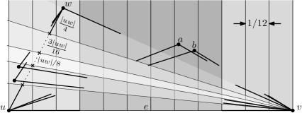
Figure 2: Sketch of the argument why no 17 points in one-sided convex position can be used to embed $K_{17}$ as a $1/4$-SHPED.

So at least eleven points of $P$ must lie in the union of the three leftmost and the three rightmost strips. We may assume that the union $S_{\mathrm{left}}$ of the three leftmost strips contains at least six points. Let $w$ be the rightmost point in $P\cap S_{\mathrm{left}}$. We subdivide the edge $uw$ into five pieces whose lengths are $1/4$, $3/16$, $1/8$, $3/16$, and $1/4$ of the length of $uw$. Each piece contains its endpoint that is closer to one of the endpoints of $uw$. The innermost piece contains both of its endpoints. Now consider the cones with apex $v$ spanned by the five pieces of $uw$. We claim that no cone contains more than one point.

Our main tool is the following. Let $t$ be a point in $(P\cap S_{\mathrm{left}})\setminus\{u,w\}$. Then the stub $tv$ intersects the right boundary of $S_{\mathrm{left}}$ and, hence, also the edge $uw$ that separates $P\cap S_{\mathrm{left}}$ from $P\setminus S_{\mathrm{left}}$. It remains to note that in each cone, any point has a stub to $u$ or $w$ (whichever is further away from the cone) that intersects the boundary of the cone. ∎

Theorem 2.1 can be used to derive a first upper bound on general point sets as follows.

Corollary 1

For any $n>\binom{30}{15}$, the graph $K_{n}$ does not admit a $1/4$-SHPED.

Proof

By a result of Erdős and Szekeres [ES35], any set of more than $\binom{2k-4}{k-2}$ points in general position contains a subset of $k$ points that form a one-sided convex set. Combining this with Theorem 2.1 and plugging in $k=17$ yields the claimed bound. ∎

We now vastly improve upon the bound of Corollary 1. Let $P$ be the point set in the plane, and let $l$ and $r$ be the two points on the convex hull that define the diameter of $P$, which is the largest distance between any two points. We rotate $P$ such that the line $lr$ is horizontal and $l$ is on the left-hand side. Now let $R$ be the smallest enclosing axis-aligned rectangle that contains $P$, and let $t$ and $b$ be the top- and bottommost points in $R$, respectively. Accordingly, let $R_{t}$ be the part of $R$ above (and including) $lr$ and let $R_{b}=R\setminus R_{t}$. We consider the two rectangles separately and assume that the interior of $R_{t}$ is not empty. (In our proof we argue, for any interior point, using only its stubs towards the three boundary points $l$, $r$, and $t$.)

We subdivide $R_{t}$ into 26 cells such that for each point in a cell the three stubs to $l$, $r$, and $t$ intersect the boundary of that cell; see Figure 3. For each cell, we prove, in the remainder of this section, an upper bound on the maximum number of points it can contain. Summing up these numbers (see again Figure 3), we get a bound of 121 points in total. Since we may have a symmetric subproblem below $lr$, we double this number, subtract 2 because of double-counting $l$ and $r$, and finally get the following theorem.

Theorem 2.2

For any $n>240$, the graph $K_{n}$ does not admit a $1/4$-SHPED.

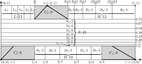
Figure 3: Partition of the enclosing rectangle $R_{t}$ into cells. We have labeled each cell or group of cells with the maximum number of points that it can contain.

We now prove Theorem 2.2 by upperbounding, for each cell in Figure 3, the number of points it contains.

For ease of presentation, we stretch $R_{t}$ in y-direction to make it a square. Clearly, this operation does not change the crossing properties. We assume that the side length of $R_{t}$ is $1$. We further assume that the coordinates of $l$, $r$, and $t$, are $(0,0)$, $(0,1)$, and $(t,1)$, respectively. Note that, by the choice of $r$ and $l$, there are no other points on the left and right boundary of $R_{t}$ (otherwise $lr$ would not be the diameter of $P$). By symmetry, we may further assume that $0<t\leq 1/2$. For a point $p$, we call stub $pt$ the upper stub of $p$, $pr$ its right stub, $pl$ its left stub, and both $pr$ and $pl$ its lower stubs.

For $p\in\{l,r,t\}$, let $C_{p}\subset R_{t}$ be the axis-parallel rectangle spanned by $p$ and the endpoints of the two stubs that go from $p$ to the two other boundary points. Note that $C_{l},C_{r}$, and $C_{t}$ (all shaded in Figure 3) are squares of size $1/4\times 1/4$.

The middle strip.

We first consider the middle strip $S=[0,1]\times[1/4,3/4]$. In order to upperbound the number of points that $S$ contains, we subdivide $S$ into eight horizontal strips, $S_{1},\dots,S_{8}$, from top to bottom. For $i=1,\dots,8$, let $a_{i}$ and $b_{i}$ be (the y-coordinates of) the lower and upper boundaries of $S_{i}$. We will fix $a_{i}$ and $b_{i}$ such that, for any point $p$ in $S_{i}$, each of $pl$, $pr$, and $pt$ intersects either $a_{i}$ or $b_{i}$.

Observe that, for any point in $S_{i}$, it holds that its lower stubs intersect $a_{i}$ if

$$3/4\cdot b_{i}\leq a_{i},$$ (1)

whereas its upper stubs intersect $b_{i}$ if

$$a_{i}+(1-a_{i})/4=(3a_{i}+1)/4\geq b_{i}.$$ (2)

We may assume that $S_{i}$ contains a point $p_{i}$ on $b_{i}$; otherwise we simply let $p_{i}$ be the topmost point in $S_{i}$ and restrict $S_{i}$ to the part between $a_{i}$ and $p_{i}$. Let

$$c_{i}=3/4\cdot b_{i}$$ (3)

be the y-coordinate where the lower stubs of points on $b_{i}$ end. We identify $c_{i}$ with the line $y=c_{i}$. For any point $p$ in $S_{i}$, let $I_{p}$ be the part of $c_{i}$ delimited by the lower stubs of $p$. Observe that, for $p,q\in S_{i}$ with $q\neq p$, it holds that $I_{p}$ and $I_{q}$ are disjoint. This is due to the fact that the upper stubs of $p$ and $q$ both intersect $b_{i}$. Let $\delta_{p}$ be the length of $I_{p}$. We say that $p$ consumes $\delta_{p}$. By the intercept theorem, we obtain that $p$ consumes $\delta_{p}/1\geq(a_{i}-c_{i})/a_{i}$ (which is what a point on $a_{i}$ would consume). The point $p_{i}$ on $b_{i}$ consumes $\delta_{p_{i}}/1=(b_{i}-c_{i})/b_{i}=1/4$; hence, the other points together can consume at most $3/4$.

To show that $S_{i}$ contains at most five points besides $p_{i}$, we choose $a_{i}$ and $b_{i}$ such that

$$6\cdot\frac{a_{i}-c_{i}}{a_{i}}\geq 3/4.$$ (4)

(The reason for allowing equality is that the left or right boundaries of $S_{i}$ do not contain any points and hence, none of the intervals on $c_{i}$ intersects the boundary of $R_{t}$.)

Combining Eqs. 3 and 4 yields $a_{i}\geq 6/7\cdot b_{i}$. This automatically implies Eq. 1, so the upper stubs of all points in $S_{i}$ intersect $b_{i}$. Additionally, we require Eq. 2 ($a_{i}\geq(4b_{i}-1)/3$) to make sure that the lower stubs of all points in $S_{i}$ intersect $a_{i}$.

Now we can fix the upper and lower boundaries of the strips. We start with $b_{1}=3/4$ and then repeatedly set $a_{i}$ to the tighter of the two lower bounds (which, for $a_{i}\leq 3/5$ is always the first one). This yields the following values:

$$\begin{array}[]{lcccl}a_{1}&=&2/3&=&b_{2},\\ a_{2}&=&4/7&=&b_{3},\\ a_{3}&=&4/7\cdot 6/7&=&b_{4},\\ a_{4}&=&4/7\cdot 6^{2}/7^{2}&=&b_{5},\\ a_{5}&=&4/7\cdot 6^{3}/7^{3}&=&b_{6},\\ a_{6}&=&4/7\cdot 6^{4}/7^{4}&=&b_{7},\\ a_{7}&=&4/7\cdot 6^{5}/7^{5}&=&b_{8},\text{ and}\\ a_{8}&=&1/4.&&\end{array}$$

So, each of the eight strips contains at most six vertices. As it turns out, we can tighten the analysis for $S_{1}$ and $S_{8}$. Each point in $S_{1}$ consumes at least $(a_{1}-c_{1})/a_{1}=5/32$. As above, all such points (except $p_{1}$) together must consume less than $3/4$. Therefore, $S_{1}$ contains at most five points. Each point in $S_{8}$ consumes $(a_{8}-c_{8})/a_{8}=24337/7^{6}\approx 0.21$; hence, $S_{8}$ contains at most four points.

Let’s summarize.

Lemma 1

The middle strip $S$ contains at most 45 points.

The middle part of the bottom strip.

We consider the rectangle $B=[1/4,3/4]\times[0,1/4]$ of length $1/2$ and height $1/4$ between the cells $C_{l}$ and $C_{r}$. Similarly as for the middle strip, we construct five cells $B_{1}$ to $B_{5}$ such that all stubs to the extreme points $r,l$ and $t$ cross the cell boundaries. We denote the left and right boundaries of cell $B_{i}$ by $a_{i}$ and $b_{i}$ and set $a_{1}=1/4$, $b_{1}=a_{2}=1/3$, $b_{2}=a_{3}=4/9$, $b_{3}=a_{4}=5/9$, $b_{4}=a_{5}=2/3$, $b_{5}=3/4$. Clearly, for every point $p$ in any cell $B_{i}$, it holds that the stubs $pl$ and $pr$ intersect the left and right boundaries $a_{i}$ and $b_{i}$, respectively. For the upper stub $pt$, we only know that it crosses the horizontal line $y=1/4$, but not necessarily the upper boundary of $B_{i}$. We say that a point $p$ is a medial point in cell $B_{i}$ if its stub $pt$ does intersect the upper boundary of $B_{i}$. We observe that no two medial points can lie in the same cell $B_{i}$ without causing stub intersections. Thus, for another point $q$ in $B_{i}$, the stub $qt$ must intersect either $a_{i}$ or $b_{i}$. We call such a point a lateral point.

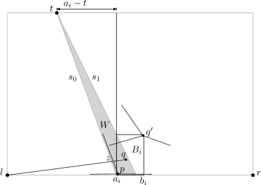
Figure 4: A cell $B_{i}$ with a medial point $q^{\prime}$ and a lateral point $p$ whose stubs do not intersect. The two lateral points $p$ and $q$ cannot both exist since the stubs $pt$ and $ql$ must intersect. (The vertical axis in this figure is scaled by $2/3$.)

In the following, we show that there can be at most one lateral point in any cell $B_{i}$. Without loss of generality, we can assume that $t<a_{i}$. We consider the two rays $s_{0}$ and $s_{1}$ from $t$ through the two corners $(a_{i},0)$ and $(a_{i},1/4)$ of $B_{i}$, see Fig. 4. These two rays define a wedge $W$. Let $p$ and $q$ be two lateral points in $B_{i}$; then $p$ and $q$ must lie in $B_{i}\cap W$. Let $p$ be the point whose ray from $t$ is left of the ray from $t$ through $q$. Then the two line segments $\overline{ql}$ and $\overline{pt}$ must intersect in a point $z$ (otherwise the stubs $pr$ and $qt$ would necessarily cross). Let $\delta_{q}=|\overline{qz}|/|\overline{zl}|$. To avoid a crossing between the stubs $pt$ and $ql$, we need that $|qz|\geq 1/4(|qz|+|zl|)$, or equivalently, that $\delta_{q}\geq 1/3$.

Using the intercept theorem, we observe that $\delta_{q}$ is maximized if $p$ lies on $s_{0}$, $q$ lies on $s_{1}$, and they both lie on the x-axis. We apply the intercept theorem once more for the line $x=a_{i}$ and the line supported by $s_{1}$ to show that in this case $|\overline{qz}|=(a_{i}-t)/3$. Using $|\overline{zl}|=a_{i}$, we get $\delta_{q}=1/3\cdot(1-t/a_{i})<1/3$. This contradicts $\delta_{q}\geq 1/3$. Thus, each cell $B_{i}$ contains at most one lateral and at most one medial point.

We summarize.

Lemma 2

The lower rectangle $B$ contains at most 10 points.

The left and the right part of the upper strip.

In the following, we consider the rectangles $L=[0,3t/4]\times[3/4,1]$ and $R=[(3t+1)/4,1]\times[3/4,1]$, separated by the upper central square $C_{t}$, which has size $1/4\times 1/4$, is adjacent to $t$, and is defined by the stubs $tl$ and $tr$. Recall that we assume $0<t\leq 1/2$.

We subdivide $R$ into five height-$1/4$ rectangles $R_{1},\dots,R_{5}$, from left to right, and analyze how many points each rectangle can contain at most. The analysis for $L$ is symmetric.

Note that the two lower stubs of any point in $R$ intersects the horizontal line $y=3/4$. To make sure that the upper stub of any point in cell $R_{i}$ intersects the left boundary with x-coordinate $a_{i}$ of $R_{i}$, the x-coordinate $b_{i}$ of the right boundary of $R_{i}$ has to fulfill $(b_{i}-t)/4\geq b_{i}-a_{i}$ and, hence, $b_{i}\leq(4a_{i}-t)/3$. (Note that we assume that the right boundary of $R_{i}$ is not part of $R_{i}$.) This yields the following boundaries.

$$\begin{array}[]{lcccl}&&3/4\cdot t+1/4&=&a_{1},\\ b_{1}&=&2/3\cdot t+1/3&=&a_{2},\\ b_{2}&=&5/9\cdot t+4/9&=&a_{3},\\ b_{3}&=&11/27\cdot t+16/27&=&a_{4},\\ b_{4}&=&17/81\cdot t+64/81&=&a_{5},\text{ and}\\ b_{5}&=&1.&&\end{array}$$

Observe that the lower stubs of all points in the same cell have to be nested: Let $p$ be a point in a cell $R_{i}$ and consider the line $s$ through $l$ and $p$. Assume there is a point $q$ above $p$ such that the lower stubs of $p$ and $q$ are not nested. Then $q$ has to be to the right of $s$. However, by the way the width of $R_{i}$ is constructed, the left stub of $q$ intersects the vertical line $a_{i}$. So, the left stub of $q$ intersects the right stub of $p$.

Now we analyze how many points can be stacked on top of each other in each subrectangle, depending on its width, its distance to $t$, and the $l$-shadow of the stub $tr$, i.e., the set of all points $p$ such that the stubs $tr$ and $pl$ intersect.

Consider first $R_{1}$. Observe that the left stub of any point $p$ in $R_{1}$ must leave $R_{1}$ through its bottom edge. Otherwise $p$ would lie in the $l$-shadow of $tr$. Hence, there are no two points with nested lower stubs in $R_{1}$. Otherwise the left stub of the upper point would intersect the upper stub of the lower point. Thus, $R_{1}$ contains at most one point.

For the remaining four subrectangles it is easy to see that they contain at most five points each. This yields to following lemma.

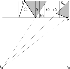
Figure 5: The lines from point $l$ to the endpoints of the stubs $tr$ and $pt$ give rise to (gray) $l$-shadows where no point can be placed.

Lemma 3

The rectangles $L$ and $R$ each contain at most 21 points.

The $(1/4\times 1/4)$-squares $C_{l}$, $C_{r}$, and $C_{t}$.

Our approach for this part follows a suggestion of Gašper Fijavž. We consider the square $C_{l}$; for the two other squares $C_{r}$ and $C_{t}$, we can argue analogously and get the same bound. Let $l,p_{1},\dots,p_{k}$ be the set of points contained in $C_{l}$.

First, we observe that the stubs from $p_{1},\dots,p_{k}$ to $t$ and $r$ intersect the upper and right boundary of $C_{l}$. Hence, the points $p_{1},\dots,p_{k}$ together with their stubs to $r$ and $t$ form a nested structure. This means that we can order the points such that, for $i=2,\dots,k$, the point $p_{i}$ lies between the stubs of $p_{i-1}$, the point $p_{k}$ being innermost. Now we define $\alpha_{1},\alpha_{2},\dots,\alpha_{k}$ to be the angles at point $r$ formed by the lines $\overline{rl}$ and $\overline{rp_{i}}$. Analogously, we have angles $\beta_{1},\dots,\beta_{k}$ at point $t$. We consider only the angles of type $\alpha_{i}$. Analogous observations hold for the angles of type $\beta_{i}$, and the resulting bounds are the same.

From the nesting, we see that the sequence $\alpha_{i}$, $i=1,\dots,k$ is monotonously increasing. Even stronger, we have the following claim.

Claim

For $1<i\leq k$ it holds that $\alpha_{i}\geq 1.3\cdot\alpha_{i-1}$.

Proof

Consider the segment from point $l$ to $p_{i}$. We subdivide it into four segments of equal length; see Fig. 7. This defines the four angles $\gamma_{1},\dots,\gamma_{4}$ by the connecting lines from point $r$. We have $\alpha_{i}=\gamma_{1}+\dots+\gamma_{4}$ and $\alpha_{i-1}\leq\gamma_{1}+\gamma_{2}+\gamma_{3}=:\gamma$. It remains to prove that $\alpha_{i}\geq 1.3\gamma$.

The ratio of $\gamma_{4}$ and $\gamma$ and, hence, the ratio of $\alpha_{i}$ and $\gamma$ is smallest if the angle $\angle r,p_{i},l$ is minimized, i.e., if $p_{i}$ lies in the upper left corner of $C_{l}$. Hence, $\alpha_{i}/\gamma\geq\arctan(1/4)/\arctan(3/16)>1.3$. Note that in general $p_{i}$ must be to the right of stub $lt$, so the ratio is even slightly better. ∎

Next, we restrict the range of the smallest and largest angle. Then we can easily compute the number $k$ of points.

Let $s$ be the endpoint of the stub $l{p_{k}}$. Consider the two lines $\overline{ts}$ and $\overline{rs}$. The point $p_{1}$, which defines the angle $\alpha_{1}$ and $\beta_{1}$ respectively, has to lie either above $\overline{rs}$ or to the right of $\overline{ts}$ or both. We assume, without loss of generality, the first case, so the angle formed by $l,r,s:=\bar{\alpha}\leq\alpha_{1}$. We call the length of the base line, which is the distance between $l$ and $r$, to be $d=1$.

Figure 6: Angles increase by a factor of at least $1.3$.

Figure 7: Ratio between the smallest and the largest angle.

We compute $\tan(\bar{\alpha})=h_{s}/d-l_{s}=(h_{k}/4)/d-l_{s}$ and $\tan(\alpha_{k})=h_{k}/(d-4l_{s})=h_{k}/(d-4l_{s})$; see Figure 7, where $h_{k}$ and $h_{s}$ are the minimum distances of $p_{k}$ and $s$, respectively, to the base line $\overline{lr}$. This yields the ratio

$$\frac{\tan\bar{\alpha}}{\tan\alpha_{k}}=\frac{h_{k}}{4(d-l_{s})}\frac{d-4l_{s}}{h_{k}}=1-\frac{3d}{4(d-l_{s})}=1-\frac{3}{4(1-l_{s}/d)}.$$

Using $l_{s}\leq(1/4)^{2}$, this yields $\tan\bar{\alpha}/\tan\alpha_{k}\geq 1/5$. From the Taylor seriesexpansion of the tangent function we know that $\tan\alpha>\alpha$, for all $0<\alpha<\pi/2$, in particular $\tan\alpha=c_{\alpha}\alpha$ with $c_{\alpha}>1$ monotonically increasing with $\alpha$.

Hence, we conclude that

$$\frac{\alpha_{1}}{\alpha_{k}}=\frac{c_{\alpha_{k}}\tan\alpha_{1}}{c_{\alpha_{1}}\tan\alpha_{k}}>\frac{\tan\bar{\alpha}}{\tan\alpha_{k}}\geq 1/5.$$

This yields $\alpha_{k}\geq(1.3)^{k-1}\cdot\alpha_{1}>(1.3)^{k-1}\cdot 1/5\cdot\alpha_{k}$, which in turn implies $k<\log 5/\log 1.3+1\leq 6.2$.

If $p_{1}$ lies to the right of $\overline{ts}$, we analogously obtain

$$\frac{\beta_{1}}{\beta_{k}}>1-\frac{3}{4(1-l_{s}/d)}$$

where $d>1$ is the distance of $l$ and $t$ and $l_{s}\leq 1/4\cdot\sqrt{2}/4$ is the length of the projection of the segment $\overline{ls}$ to the line $lt$, hence $\beta_{1}>1/6\cdot\beta_{k}$.

Arguing along the lines of the first case, we get $\beta_{k}>(1.3)^{k-1}\cdot 1/6\cdot\beta_{k}$, and derive $k<7.9$.

Lemma 4

The squares $C_{l}$, $C_{t}$, and $C_{r}$ each contain at most eight points.

This finishes the proof of Theorem 2.2.

3 Improved Bounds for Specific Graph Classes

In this section, we improve, for specific graph classes, the result of Bruckdorfer and Kaufmann [BK12] which says that $K_{n}$ (and thus, any $n$-vertex graph) has a $1/\sqrt{4n/\pi}$-SHPED. In other words, $K_{n}$ has a $\delta$-SHPED if $n\leq\pi/(4\delta^{2})$. We give two constructions for complete bipartite graphs and one for graphs of bounded bandwidth.

Complete Bipartite Graphs.

Our first construction is especially suitable if both sides of the bipartition have about the same size. The drawing is illustrated in Figure 8a. Note that in the figure the x- and y-axes are scaled differently.

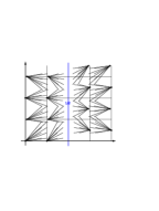
(a) $1/4$-SHPED of $K_{8,8}$

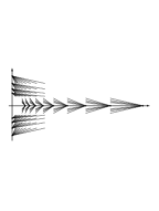
(b) $1/4$-SHPED of $K_{8,9}$

Figure 8: Two methods for drawing complete bipartite graphs as SHPEDs.

Theorem 3.1

The complete bipartite graph $K_{n,n}$ has a $\delta$-SHPED if

$$n\leq\left\lfloor\frac{1}{\delta}\right\rfloor\cdot\left\lfloor\left\lfloor\frac{\log 1/2}{\log(1-\delta)}\right\rfloor\right\rfloor,$$

where $\lfloor\lfloor r\rfloor\rfloor$ denotes the largest integer that is strictly less than $r$.

Proof

Let $k=\left\lfloor\frac{1}{\delta}\right\rfloor$ and $\ell=\left\lfloor\left\lfloor\frac{\log 1/2}{\log(1-\delta)}\right\rfloor\right\rfloor$. The latter implies that $(1-\delta)^{\ell}>\frac{1}{2}$.

Divide the plane at the vertical line $x=1/2$ into two half planes, one for each side of the bipartition, to which we will refer as the right-hand side and the left-hand side. In each half plane draw the $n$ vertices on a (perturbed) $k\times\ell$ grid. More precisely, for a horizontal line, let $\epsilon\geq 0$ such that $(1-\delta)^{\ell}>\frac{1}{2}+\epsilon$. Draw the vertices with x-coordinates

$$(1-\delta)^{i}-\epsilon\text{ and }1-(1-\delta)^{i}+\epsilon,i=0,\dots,\ell-1.$$

Draw the vertices on the left-hand side with y-coordinates $0,\dots,k-1$ and the vertices on the right-hand side with y-coordinates $0+\sigma,\dots,k-1+\sigma$ where $0<\sigma<1$ is chosen such that no two vertices on the right-hand side are collinear with a vertex on the left-hand side and vice versa. All edges are between a vertex on the left-hand side and a vertex on the right-hand side.

Then for any two vertices the bounding boxes of their incident stubs are disjoint up to their boundaries. Intersections of the stubs on the boundaries can be avoided by a suitable choice of $\epsilon$.

1. If $v$ is a vertex on the right-hand side with x-coordinate $(1-\delta)^{i}-\epsilon$. Then the projection to the x-axis of the longest edge incident to $v$ has length $(1-\delta)^{i}-\epsilon$. Hence all stubs incident to $v$ are in the vertical strip bounded by $x=(1-\delta)^{i}-\epsilon$ and $x=(1-\delta)^{i}-\epsilon-\delta((1-\delta)^{i}-\epsilon)\geq(1-\delta)^{i+1}-\epsilon>1/2$. The latter inequation follows since $i+1\leq\ell$.

2. Let $v_{i}$ be a vertex with y-coordinate $\sigma+i$, $i=0,\dots,k-1$. Then the projection to the y-axis of the longest edge incident to $v_{i}$ and above $v$ has length $k-1-i-\sigma$ while the projection to the y-axis of the longest edge incident to $v_{i}$ and below $v$ has length $i+\sigma$. Hence the projection to the y-axis of the stubs incident to $v_{i}$ and $v_{i+1}$ do not intersect if $\delta(k-1-i-\sigma)+\delta(i+1+\sigma)<1$ which is fulfilled if $k<1/\delta$. If $k=1/\delta$ then draw the vertices on the horizontal lines $y=i$ and $y=i+\sigma$ for even $i$ with $\epsilon=0$ and the vertices on the other horizontal lines with a slightly positive $\epsilon$ such that the end points of the stubs do not intersect.

A symmetric argument holds for the vertices on the left-hand side. ∎

Our second construction is especially suitable if one side of the bipartition is much larger than the other. The drawing is illustrated in Figure 8b.

Theorem 3.2

For any integers $n>0$ and $k<{\log\delta}/{\log(1-\delta)}$, the complete bipartite graph $K_{2k,n}$ has a $\delta$-SHPED.

Proof

Draw the $n$ vertices on the x-axis with x-coordinate $x_{i}=1/(1-\delta)^{i-1},i=1,\dots,n$ and the $2k$ vertices on the y-axis with y-coordinate $y_{i}=1/(1-\delta)^{i-1},i=1,\dots,k$ and $-y_{i},i=1,\dots,k$. All edges are between a vertex on the y-axis and a vertex on the x-axis. To show that no stubs intersect, we establish the following two properties on the regions that contain the stubs.

1. The stubs incident to $(0,\pm y_{i}),i=2,\dots,k$ are in the horizontal strip bounded by $y=\pm y_{i}$ and $y=\pm y_{i-1}$:

   The projection to the y-axis of any stub incident to $(0,y_{i})$ has length $\delta\cdot y_{i}$, hence it stops at $y=(1-\delta)\cdot\left(\frac{1}{1-\delta}\right)^{i-1}=\left(\frac{1}{1-\delta}\right)^{i-2}=y_{i-1}$.

2. The stubs incident to $(0,x_{i}),i=2,\dots,n$ are in the rectangle bounded by $y=\pm(1-\delta)$, $x=x_{i-1}$, and $x=x_{i}$ (where $x_{0}=1-\delta$):

   As above, the projection of any stub incident to $(0,x_{i})$ stops at $x=x_{i-1}$. The absolute value of the projection to the y-axis is bounded by $\delta\cdot y_{k}=\delta\cdot\left(\frac{1}{1-\delta}\right)^{k-1}$ which is less than $1-\delta$ if $k<{\log\delta}/{\log(1-\delta)}$.

Since the stubs incident to $(0,\pm y_{1})$ lie in the horizontal strip bounded by $y=\pm 1$ and $y=\pm(1-\delta)$, it follows that any two stubs are disjoint. ∎

Graphs of Bounded Bandwidth.

Recall that the $k$-circulant graph $C_{n}^{k}$ with $n$ vertices and $0\leq k<n$ is the undirected simple graph whose vertex set is $\{v_{0},\dots,v_{n-1}\}$ and whose edge set is $\{v_{i}v_{j}\colon|j-i|\leq k\}$. When we specify the index of a vertex, we implicitly assume calculation modulo $n$. Note that $C_{n}^{1}=C_{n}$ and $C_{n}^{n/2}=K_{n}$. We provide $\delta$-SHPED constructions for $k$-circulant and bandwidth-$k$ graphs where $\delta=\Theta\big{(}1/\sqrt{k}\,\big{)}$. For ease of presentation, we assume that $\sqrt{k}$ and $n\big{/}\sqrt{k}$ are integers.

First, let $G$ be a graph of bandwidth $k$, i.e., the vertices of $G$ can be ordered $v_{1},\dots,v_{n}$ and for each edge $v_{i}v_{j}$ it holds that $|j-i|\leq k$. We draw $G$ as a $\delta$-SHPED as follows. We map the vertices of $G$ to the vertices of an integer grid of $\big{(}n\big{/}\sqrt{k}\times\sqrt{k}\,\big{)}$ points such that the sequence of vertices $v_{1},\dots,v_{n}$ traverses the grid column by column in a snake-like fashion, see Figure 9a.

The distance from any vertex to its $k$-th successor is at most $\sqrt{\big{(}\sqrt{k}-1\big{)}^{2}+k}<\sqrt{2k}$, see the two dashed line segments in Figure 9a. Setting $\delta=1/\big{(}2\sqrt{2k}\,\big{)}$ ensures that each stub is contained in the radius-$1/2$ disks centered at the vertex to which it is incident; see Figure 9a. Since the disks are pairwise disjoint, so are the stubs.

For the $k$-circulant graph $C_{n}^{k}$, we modify this approach such that start and end of the snake coincide. In other words, we deform our rectangular section of the integer grid into an annulus; see Figure 9b. We additionally assume that $n/\sqrt{k}$ is even.

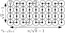
(a) path case

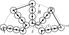
(b) circle case

Figure 9: SHPEDs for bandwidth-$k$ and $k$-circulant graphs.

The inner circle circumscribes a regular $\big{(}n/\sqrt{k}\,\big{)}$-gon $\Pi$ of edge length 1.

We place the vertices of $C_{n}^{k}$ on rays that go from the center of the annulus through the vertices of $\Pi$. On each ray, we place $\sqrt{k}$ vertices at distance 1 from one another, starting from the inner circle and ending at the outer circle. The sequence again traverses the stacks of vertices in a snake-like fashion.

A vertex $v$ can be reached from its $j$-th ($j<k$) successor $s$, by traversing at most $3\sqrt{k}-2$ segments of length 1: at most $\sqrt{k}-1$ segments from $s$ to the inner circle, at most $\sqrt{k}$ segments on the inner circle, and at most $\sqrt{k}-1$ segments from the inner circle to $v$. Hence, the maximum distance of two adjacent vertices is less than $3\sqrt{k}$, and we can choose $\delta=1/(6\sqrt{k})$.

Theorem 3.3

Let $2\leq k\leq n$ and assume that $\sqrt{k}$ and $n\big{/}\sqrt{k}$ are integers. Then any graph of bandwidth $k$ has a $1\big{/}\big{(}2\sqrt{2k}\,\big{)}$-SHPED. If additionally $n\big{/}\sqrt{k}$ is even, the $k$-circulant graph $C_{n}^{k}$ has a $1\big{/}\big{(}6\sqrt{k}\,\big{)}$-SHPED.

4 Geometrically Embedded SPEDs

Bruckdorfer and Kaufmann [BK12] gave an integer-linear program for MaxSPED and conjectured that the problem is NP-hard. Indeed, there is a simple reduction from Planar3SAT [KS12]. In this section, we first show that the problem can be solved efficiently for the special case of graphs that admit a 2-planar geometric embedding. Then we turn to the dual problem MinSPED of minimizing the ink that has to be erased in order to turn a given drawing into a SPED.

4.1 Maximizing Ink in Drawings of 2-Planar Graphs

In this section we prove that, given a 2-planar geometric embedding $\Gamma$ of a 2-planar graph $G$ with $n$ vertices, we can compute a maxSPED, i.e., a SPED that maximizes the total stub length, in $O(n\log n)$ time. Recall that a graph $G$ is 2-planar if it admits a simple drawing on the plane where each edge is crossed at most twice.

Given $G$ and $\Gamma$, we define a simple undirected graph $C$ as follows. $C$ has a vertex $v_{e}$ for each edge $e$ of $G$. Two vertices $v_{e}$ and $v_{e^{\prime}}$ of $C$ are connected by an edge if and only if $e$ and $e^{\prime}$ form a crossing in $\Gamma$. Such a graph is in general non-connected. Furthermore, since the maximum degree of $C$ is $2$, a connected component of $C$ is either a path (possibly formed by only one edge) or a cycle.

Let $C_{i}$ be a connected component of $C$. We define a total ordering of the vertices of $C_{i}$. Namely, if $C_{i}$ is a path such an ordering is directly defined by the order of its vertices along the path (rooted at an arbitrary end vertex). If $C_{i}$ is a cycle, we simply delete an arbitrary edge of the cycle, obtaining again a path and the related order. That means, if we consider the subdrawing $\Gamma_{i}$ of $\Gamma$ induced by the vertices of $C_{i}$ (edges of $G_{i}$), such a drawing is formed by an ordered sequence of edges (according to the ordering of the vertices of $C_{i}$), $e_{1},\dots,e_{n_{i}}$, such that $e_{j}$ crosses $e_{(j+1)\bmod n_{i}}$ for $j=1,\dots,n_{i}-1$ in case of a path, and $j=1,\dots,n_{i}$ in case of a cycle.

We will use the following notation: $l_{j}$ is the total length of the edge $e_{j}$; $x_{j}^{\prime}$ is the length of the shortest stub of $e_{j}$ defined by the crossing between $e_{j-1}$ and $e_{j}$, called the backward stub; $x_{j}^{\prime\prime}$ is the length of the shortest stub of $e_{j}$ defined by the crossing between $e_{j}$ and $e_{j+1}$, called the forward stub. See also Figure 10.

Figure 10: Notation used in the DP.

Consider now the subdrawing $\Gamma_{i}$, and assume that $e_{1},\dots,e_{n_{i}}$ form a path in $C_{i}$. If $n_{i}=2$, the maximum total length of the stubs is $k_{\mathrm{opt}}=\max\{l_{1}+2x_{2}^{\prime},l_{2}+2x_{1}^{\prime\prime}\}$.

In the general case, we can process the path edge by edge, having at most three choices for each edge: $(i)$ we can draw it entirely, $(ii)$ we can draw only its backward stubs, or $(iii)$ we can draw only its forward stubs. The number of choices we have at any step is influenced only by the previous step, while the best choice is determined only by the rest of the path. Following this approach, let $\gamma_{i}$ be a maxSPED for $\Gamma_{i}$ and consider the choice done for the first edge $e_{1}$ of the path. The total length of the stubs in $\gamma_{i}$, minus the length of the stubs assigned to $e_{1}$, represents an optimal solution for $\Gamma_{i}\setminus e_{1}$, under the initial condition defined by the first step, otherwise, $\gamma_{i}$ could be improved, a contradiction. I.e., the optimality principle holds for our problem. Thus, we can exploit the following dynamic programming (DP) formulation, where $O_{\mathrm{in}}(e_{j})$ describes the maximum total length of the stubs of $e_{j},\dots,e_{n_{i}}$ under the choice $(i)$ for $e_{j}$, $O_{\mathrm{out}}^{\prime}(e_{j})$ describes the choice $(ii)$ and $O_{\mathrm{out}}^{\prime\prime}(e_{j})$ describes the choice $(iii)$.

$$O_{\mathrm{in}}(e_{j}) =\begin{cases}l_{j}+\max\{O_{\mathrm{out}}^{\prime}(e_{j+1}),O_{\mathrm{out}}^{\prime\prime}(e_{j+1})\}&\text{if $x_{j+1}^{\prime}\geq x_{j+1}^{\prime\prime}$,}\\ l_{j}+O_{\mathrm{out}}^{\prime}(e_{j+1})&\text{if $x_{j+1}^{\prime}<x_{j+1}^{\prime\prime}$.}\end{cases}$$ (5a)

$$O_{\mathrm{out}}^{\prime}(e_{j}) =\begin{cases}2x_{j}^{\prime}+\max\{O_{\mathrm{out}}^{\prime}(e_{j+1}),O_{\mathrm{out}}^{\prime\prime}(e_{j+1})\}&\text{if $x_{j}^{\prime}>x_{j}^{\prime\prime}$ and $x_{j+1}^{\prime}\geq x_{j+1}^{\prime\prime}$,}\\ 2x_{j}^{\prime}+O_{\mathrm{out}}^{\prime}(e_{j+1})&\text{if $x_{j}^{\prime}>x_{j}^{\prime\prime}$ and $x_{j+1}^{\prime}<x_{j+1}^{\prime\prime}$,}\\ \lx@intercol 2x_{j}^{\prime}+\max\{O_{\mathrm{in}}(e_{j+1}),O_{\mathrm{out}}^{\prime}(e_{j+1}),O_{\mathrm{out}}^{\prime\prime}(e_{j+1})\}\qquad\quad\;\;\;\text{if $x_{j}^{\prime}\leq x_{j}^{\prime\prime}$.}\hfil\lx@intercol\end{cases}$$ (5b)

$$O_{\mathrm{out}}^{\prime\prime}(e_{j}) =2x_{j}^{\prime\prime}+\max\{O_{\mathrm{in}}(e_{j+1}),O_{\mathrm{out}}^{\prime}(e_{j+1}),O_{\mathrm{out}}^{\prime\prime}(e_{j+1})\}$$ (5c)

In case of a path, we store in a table the values of $O_{\mathrm{in}}(e_{j})$, $O_{\mathrm{out}}^{\prime}(e_{j})$ and $O_{\mathrm{out}}^{\prime\prime}(e_{j})$, for $j=1,\dots,n_{i}$, through a bottom-up visit of the path (from $e_{n_{i}}$ to $e_{1}$). Since $e_{1}$ and $e_{n_{i}}$ do not cross, we have $x_{1}^{\prime}=l_{1}/2$ and $x_{n_{i}}^{\prime\prime}=l_{n_{i}}/2$. Then, the maximal value of ink is given by $k_{\mathrm{opt}}=\max\{O_{\mathrm{in}}(e_{1}),O_{\mathrm{out}}^{\prime}(e_{1}),O_{\mathrm{out}}^{\prime\prime}(e_{1})\}$. See Figure 11 for an example.

In case of a cycle, we have that $e_{1}$ and $e_{n_{i}}$ cross each other, thus, in order to compute the table of values we must assume an initial condition for $e_{n_{i}}$. Namely, we perform the bottom-up visit from $e_{n_{i}}$ to $e_{1}$ three times. The first time we consider as initial condition that $e_{n_{i}}$ is entirely drawn (choice $O_{\mathrm{in}}(e_{n_{i}})$), the second time we consider only the backward stubs drawn (choice $O_{\mathrm{out}}^{\prime}(e_{n_{i}})$), and the third time we consider only the forward stubs drawn (choice $O_{\mathrm{out}}^{\prime\prime}(e_{n_{i}})$). Every initial condition will lead to a table where, in general, we do not have all the three possible choices for $e_{1}$ (i.e., some choices are forbidden due to the initial condition). Performing the algorithm for every possible initial condition and choosing the best value yields the optimal solution $k_{\mathrm{opt}}$.

(a)

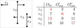
(b)

Figure 11: (a) A 2-planar drawing $\Gamma$ and (b) a maxSPED of $\Gamma$ computed by the DP algorithm.

The algorithm described above leads to the following result.

Theorem 4.1

Let $G$ be a graph with $n$ vertices, and let $\Gamma$ be a 2-planar geometric embedding of $G$. A maxSPED of $\Gamma$ can be computed in $O(n\log n)$ time.

Proof

Consider the above described algorithm, based on the DP formulation defined by the set of equations (5). We already showed how this algorithm computes a maxSPED of $\Gamma$. The construction of the graph $C$ requires time $O(m\log m)$ with a standard sweep-line algorithm for computing the $O(m)$ line-segment intersections [BO79]. Once $C$ has been constructed, ordering its vertices requires $O(n_{C})$ time, where $n_{C}\in O(m)$ is the number of vertices of $C$. Performing a bottom-up visit and up to three top-down visits of every path or cycle takes $O(m)$ time. Thus, the overall time complexity is $O(n\log n)$, since for 2-planar graphs $m\in O(n)$ [PT97]. ∎

We finally observe that the restricted $0/1$-MaxSPED problem for 2-planar drawings, where each edge is either drawn or erased completely, may be solved through a different approach. Indeed, we can exploit a maximum-weight SAT formulation in the CNF+($\leq$2) model, where each variable can appear at most twice and only with positive values [PS07]. Roughly speaking, we map each edge to a variable, with the weight of the variable equal to the length of its edge, and define a clause for each crossing. Applying an algorithm of Porschen and Speckenmeyer [PS07] for CNF+($\leq$2) solves $0/1$-MaxSPED in $O(n^{3})$ time. However, our algorithm solves a more general problem in less time.

4.2 Erasing Ink in Arbitrary Graph Drawings

In this section, we consider the problem MinSPED, which is dual to MaxSPED. In MinSPED, we are given a graph with a straight-line drawing (i.e., a geometric graph), and the task is to erase as little of the edges as possible in order to make it a SPED.

We will exploit a connection between the NP-hard minimum-weight 2-SAT problem (MinW2Sat) and MinSPED. Recall that MinW2Sat, given a 2-SAT formula, asks for a satisfying variable assignment that minimizes the total weight of the true variables. There is a 2-approximation algorithm for MinW2Sat that runs in $O(vc)$ time and uses $O(c)$ space, where $v$ is the number of variables and $c$ is the number of clauses of the given 2-SAT formula [BYR01].

Theorem 4.2

MinSPED can be 2-approximated in time quadratic in the number of crossings of the given geometric graph.

Proof

Given an instance $G$ of MinSPED, we construct an instance $\varphi$ of MinW2Sat as follows. Let $e$ be an edge of $G$ with $k$ crossings. Then $e$ is split into $k+1$ pairs of edge segments $e_{0},\dots,e_{k}$ as shown in Figure 12. If we order the edges that cross $e$ in increasing order of the distance of their crossing point to the closer endpoint of $e$, we can assign each segment pair $e_{i}$ for $i\geq 1$ to the $i$th edge $f^{i}$ crossing $e$, in this order. We also say that edge $f^{i}$ induces segment pair $e_{i}$. Any valid maximal (non-extensible) partial edge drawing of $e$ is the union $\bigcup_{i=0}^{j}e_{i}$ of all pairs of edge segments up to some index $j\leq k$.

Figure 12: Edge $e$ is split into four pairs of edge segments; pairs are labeled equally.

We model all pairs of (induced) edge segments as truth variables $\hat{e}_{1},\dots,\hat{e}_{k}$ with the interpretation that the pair $e_{i}$ is not drawn if $\hat{e}_{i}=\mathit{true}$. The pair $e_{0}$ is always drawn. For $i=1,\dots,k$, we introduce the clause $(\neg\hat{e}_{i+1}\Rightarrow\neg\hat{e}_{i})\equiv(\hat{e}_{i+1}\lor\neg\hat{e}_{i})$. This models that $e_{i+1}$ can only be drawn if $e_{i}$ is drawn. Moreover, for every crossing between two edges $e$ and $f$, we introduce the clause $(e_{i}\lor f_{j})$, where $e_{i}$ is the segment pair of $e$ induced by $f$ and $f_{j}$ is the segment pair of $f$ induced by $e$. This simply means that at least one of the two induced segment pairs is not drawn and thus the crossing is avoided.

Now we assign a weight $w_{e,i}$ to each variable $\hat{e}_{i}$, which is either the absolute length $|e_{i}|$ of $e_{i}$ if we are interested in ink, or the relative length $|e_{i}|/(2|e|)$ if we are interested in relative stub lengths ($\delta$). Then minimizing the value $\sum_{\hat{e}_{i}\in\text{Var}(\varphi)}w_{e,i}\hat{e}_{i}$ over all valid variable assignments minimizes the weight of the erased parts of the edges in the given geometric graph

The 2-approximation algorithm for MinW2Sat yields a 2-approximation for the problem to erase the minimum ink from the given straight-line drawing of $G$. It runs in $O(vc)=O(I^{2})\subseteq O(m^{4})$ time since our 2-SAT formula has $O(I)\subseteq O(m^{2})$ variables and clauses, where $m$ is the number of edges of $G$ and $I$ is the number of intersections in the drawing of $G$. ∎

If we encode the primal problem (maximize ink) using 2SAT, we cannot hope for a similar positive result. The reason is that the tool that we would need, namely an algorithm for the problem MaxW2Sat dual to MinW2Sat would also solve maximum independent set (MIS). For MIS, however, no $(n^{1-\varepsilon})$-approximation exists unless ${\cal NP}={\cal ZPP}$ [Hås99].

To see that MaxW2Sat can be used to encode MIS, use a variable $\hat{v}$ for each vertex $v$ of the given (graph) instance $G$ of MIS and, for each edge $\{u,v\}$ of $G$, the clause $(\hat{u}\vee\hat{v})$. Let $\varphi$ be the conjunction of all such clauses. Then finding a satisfying truth assignment for $\varphi$ that maximizes the number of false variables (i.e., all variable weights are 1) is equivalent to finding a maximum independent set in $G$. Note that this does not mean that maximizing ink is as hard to approximate as MIS.

Acknowledgments. We thank Ferran Hurtado and Yoshio Okamoto for invaluable pointers to results in discrete geometry. We thank Emilio Di Giacomo, Antonios Symvonis, Henk Meijer, Ulrik Brandes, and Gašper Fijavž for helpful hints and intense discussions. We thank Jarek Byrka for the link between ink maximization and MIS. Thanks to Thomas van Dijk for drawing Figure 1 (and implementing the ILP behind it).

References

- [BEW95] Richard A. Becker, Stephen G. Eick, and Allan R. Wilks. Visualizing network data. IEEE Trans. Visual. Comput. Graphics, 1(1):16–28, 1995.
- [BK12] Till Bruckdorfer and Michael Kaufmann. Mad at edge crossings? Break the edges! In Evangelos Kranakis, Danny Krizanc, and Flaminia Luccio, editors, Proc. 6th Int. Conf. Fun with Algorithms (FUN’12), volume 7288 of LNCS, pages 40–50. Springer-Verlag, 2012.
- [BO79] J. L. Bentley and T. A. Ottmann. Algorithms for reporting and counting geometric intersections. IEEE Trans. Comput., 28(9):643–647, 1979.
- [BVKW12] Michael Burch, Corinna Vehlow, Natalia Konevtsova, and Daniel Weiskopf. Evaluating partially drawn links for directed graph edges. In Marc van Kreveld and Bettina Speckmann, editors, Proc. 19th Int. Symp. Graph Drawing (GD’11), volume 7034 of LNCS, pages 226–237. Springer-Verlag, 2012.
- [BYR01] R. Bar-Yehuda and D. Rawitz. Efficient algorithms for integer programs with two variables per constraint. Algorithmica, 29:595–609, 2001.
- [DEGM05] Matthew Dickerson, David Eppstein, Michael T. Goodrich, and Jeremy Yu Meng. Confluent drawings: Visualizing non-planar diagrams in a planar way. J. Graph Algorithms Appl., 9(1):31–52, 2005.
- [ES35] Paul Erdős and G. Szekeres. A combinatorial problem in geometry. Compositio Mathematica, 2:463–470, 1935.
- [EvKMS09] David Eppstein, Marc van Kreveld, Elena Mumford, and Bettina Speckmann. Edges and switches, tunnels and bridges. Comput. Geom. Theory Appl., 42(8):790–802, 2009.
- [GHNS11] Emden R. Gansner, Yifan Hu, Stephen C. North, and Carlos Eduardo Scheidegger. Multilevel agglomerative edge bundling for visualizing large graphs. In Giuseppe Di Battista, Jean-Daniel Fekete, and Huamin Qu, editors, Proc. 4th IEEE Pacific Visual. Symp. (PacificVis’11), pages 187–194, 2011.
- [Hås99] Johan Håstad. Clique is hard to approximate within . Acta Math., 182:105–142, 1999.
- [HvW09] Danny Holten and Jarke J. van Wijk. Force-directed edge bundling for graph visualization. Comput. Graphics Forum, 28(3):983–990, 2009.
- [KS12] Philipp Kindermann and Joachim Spoerhase. Private communication, March 2012.
- [PLCP12] Dichao Peng, Neng Lu, Wei Chen, and Qunsheng Peng. SideKnot: Revealing relation patterns for graph visualization. In Helwig Hauser, Stephen G. Kobourov, and Huamin Qu, editors, Proc. 5th IEEE Pacific Visual. Symp. (PacificVis’12), pages 65–72, 2012.
- [PS07] Stefan Porschen and Ewald Speckenmeyer. Algorithms for variable-weighted 2-SAT and dual problems. In João Marques-Silva and Karem Sakallah, editors, Proc. 10th Int. Conf. Theory Appl. Satisfiability Testing (SAT’07), volume 4501 of LNCS, pages 173–186. Springer-Verlag, 2007.
- [PT97] János Pach and Géza Tóth. Graphs drawn with few crossings per edge. Combin., 17:427–439, 1997.
- [RFJR11] Amalia Rusu, Andrew J. Fabian, Radu Jianu, and Adrian Rusu. Using the gestalt principle of closure to alleviate the edge crossing problem in graph drawings. In Proc. 15th Int. Conf. Inform. Visual. (IV’11), pages 488–493, 2011.