Behavior of a Model Dynamical System with Applications to Weak Turbulence

Abstract.

We experimentally explore solutions to a model Hamiltonian dynamical system recently derived to study frequency cascades in the cubic defocusing nonlinear Schrödinger equation on the torus. Our results include a statistical analysis of the evolution of data with localized amplitudes and random phases, which supports the conjecture that energy cascades are a generic phenomenon. We also identify stationary solutions, periodic solutions in an associated problem and find experimental evidence of hyperbolic behavior. Many of our results rely upon reframing the dynamical system using a hydrodynamic formulation.

1. Introduction

Recent investigations in [4] reduced the study of the nonlinear Schrödinger equation (NLS),

(1.1) $$iu_{t}+\Delta u-|u|^{2}u=0,\ \ u(0,x)=u_{0}(x)\ \text{for}\ x\in\mathbb{T}^{2},$$

to the “Toy Model” dynamical system given by the equation

(1.2) $$-i\partial_{t}b_{j}(t)=-\lvert b_{j}(t)\rvert^{2}b_{j}(t)+2b_{j-1}^{2}\overline{b_{j}}(t)+2b_{j+1}^{2}\overline{b_{j}}(t)$$

for $j=1,\ldots,N$, with boundary conditions

(1.3) $$b_{0}(t)=b_{N+1}(t)=0.$$

The $b_{j}$’s approximate the energy of families of resonantly interacting frequencies to be described below. The main purpose of this paper is to study the evolution equation (1.2), both to gain additional insight into (1.1) and for its own sake.

In addition to showing how (1.2) approximates (1.1), a key result of [4] is the construction of a solution to (1.2) which transfers mass from low index $j$ to high $j$. In the underlying NLS problem, this implies there exist arbitrarily large, but finite, energy cascades. Thus, [4] showed that Hamiltonian dispersive equations posed on tori can have “weakly turbulent dynamics,” the phenomenon by which arbitrarily high index Sobolev norms can grow to be arbitrarily large in finite time.

The question of energy cascades in infinite dimensional dynamical systems was considered by Bourgain [2], who asked if there was a solution to (1.1) with an initial condition $u_{0}\in H^{s}$, $s>1$, such that

(1.4) $$\limsup_{t\to\infty}\|u(t)\|_{H^{s}}=\infty.$$

This corresponds to a weakly turbulent dynamic, as there is growth in high Sobolev norms, but no finite time singularity. Indeed, since (1.1) is defocusing it has a bounded $H^{1}$ norm. One can view this behavior as an “infinite-time blowup.”

Although the result in [4] does not answer Bourgain’s question, it makes significant progress. The result says that given a threshold $K\gg 1$ and $\delta>0$ there exists $u_{0}\in H^{s}$ with $\|u_{0}\|_{H^{s}}\leq\delta$ and $T>0$ such that $\|u(T)\|_{H^{s}}\geq K$, where $u$ is the solution to the NLS with $u(0)=u_{0}$. This establishes

(1.5) $$\inf_{\delta>0}\bigg{\{}\limsup_{t\to\infty}\Big{(}\sup_{\|u_{0}\|_{H^{s}}\leq\delta}\|u(t)\|_{H^{s}}\Big{)}\bigg{\}}=\infty,$$

but not (1.4). This is one of the first rigorous result exhibiting the shift of energy from low to high frequencies for a nonlinear Hamiltonian PDE viewed as an infinite-dimensional Hamiltonian dynamical system, see also work by Kuksin [9]. The works Carles-Faou [3], Hani [7], and Guardia-Kaloshin [6] have also recently treated (1.1). A particular achievement of these newer works is their careful construction of error estimates on the non-resonant terms.

The dynamics in [4] were not shown to be generic. Rather, the authors constructed a single solution with the desired properties. The stability of this solution to the flow (1.2) is unknown. One purpose of this note is to explore this question of “genericity”, by investigating ensembles of data for (1.2), and finding that, on average, there is a transfer of energy from low to high indices.

In addition to this statistical study, we seek out other interesting dynamics in (1.2). Notable behaviors we found include:

• Compactly supported, time harmonic, structures;

• Spatially and temporally periodic solutions subject to the adoption of periodic boundary conditions,

  (1.6) $$b_{0}(t)=b_{N}(t),\quad b_{N+1}(t)=b_{1}(t);$$

• Nonlinear hyperbolic behavior with both rarefactive waves and dispersive shock waves.

Many of these solutions are obtained by going to the hydrodynamic formulation of the problem. Making the Madelung transformation,

(1.7) $$b_{j}(t)=\sqrt{\rho_{j}(t)}\exp(i\phi_{j}(t))$$

with $\rho_{j}\geq 0$ and $\phi_{j}\in\mathbb{R}$, we obtain evolution equations for $\rho_{j}$ and $\phi_{j}$:

(1.8a) $$\dot{\phi}_{j} =-\rho_{j}+2\rho_{j-1}\cos\left[2(\phi_{j-1}-\phi_{j})\right]+2\rho_{j+1}\cos\left[2(\phi_{j+1}-\phi_{j})\right],$$

(1.8b) $$\dot{\rho}_{j} =-4\rho_{j}\rho_{j-1}\sin\left[2(\phi_{j-1}-\phi_{j})\right]-4\rho_{j}\rho_{j+1}\sin\left[2(\phi_{j+1}-\phi_{j})\right].$$

From this perspective, it is clear that phase interactions play a key role in the dynamics.

2. Properties of the Toy Model

In this section, we briefly review the connection between (1.1) and (1.2), and review some important structural properties of (1.2).

2.1. Relationship to NLS

First, we summarize the argument from [4] which relates NLS to the Toy Model. This begins by studying NLS in Fourier space,

$$u(t,x)=\sum_{n\in\mathbb{Z}^{2}}a_{n}(t)e^{in\cdot x+|n|^{2}t}.$$

After a choice of gauge eliminating certain trivial interactions, the Fourier amplitudes $\{a_{n}\}$ are seen to evolve according to

(2.1) $$-i\partial_{t}a_{n}=-a_{n}|a_{n}|^{2}+\sum_{n_{1},n_{2},n_{3}\in\Gamma(n)}a_{n_{1}}\bar{a}_{n_{2}}a_{n_{3}}e^{i\omega_{4}t},$$

where

$$\omega_{4}=|n_{1}|^{2}-|n_{2}|^{2}+|n_{3}|^{2}-|n|^{2},$$

$$\Gamma(n)=\left\{(n_{1},n_{2},n_{3})\in(\mathbb{Z}^{2})^{3}|n_{1}-n_{2}+n_{3}=n,\ n_{1}\neq n,\ n_{3}\neq n\right\}.$$

For any $n$, the most significant contributions in the summation will be the elements of $\Gamma(n)$ belonging to the resonant set,

$$\Gamma_{\rm res}(n)=\left\{(n_{1},n_{2},n_{3})\in\Gamma(n)\mid|n_{1}|^{2}-|n_{2}|^{2}+|n_{3}|^{2}-|n|^{2}=0\right\}.$$

Restricting (2.1) to the resonant modes, we have

(2.2) $$-i\partial_{t}r_{n}=-r_{n}|r_{n}|^{2}+\sum_{n_{1},n_{2},n_{3}\in\Gamma_{\rm res}(n)}r_{n_{1}}\bar{r}_{n_{2}}r_{n_{3}}.$$

A union of disjoint sets, $\Lambda_{j}$, of resonantly interacting frequencies is constructed,

$$\boldsymbol{\Lambda}=\Lambda_{1}\cup\Lambda_{2}\cup\cdots\cup\Lambda_{N},$$

where the mass from modes in generation $\Lambda_{j}$, $r_{n_{1}}$ and $r_{n_{3}}$, can mix to transfer mass to modes $r_{n}$ and $r_{n_{2}}$ in generation $\Lambda_{j+1}$, where again $n_{1}-n_{2}+n_{3}=n$. Subject to certain additional conditions, we will have that for all $t$ and $j$,

$$r_{n}(t)=r_{n^{\prime}}(t),\quad\forall\ n,n^{\prime}\in\Lambda_{j}.$$

Once these sets have been constructed, a nontrivial step, the relationship between the toy model and (2.2) is

(2.3) $$b_{j}(t)=r_{n}(t),\quad\forall\ n\in\Lambda_{j}.$$

Hence, $\lvert b_{j}(t)\rvert^{2}$ is a measure of the spectral energy density of generation $\Lambda_{j}$.

To show that NLS has an energy cascade, the authors used ideas inspired from studies of Arnold diffusion (see [1]) and explicit ODE manipulations to show that the Toy Model admits an instability mechanism transferring mass from a low index node to a high index node. By the construction of the initial data set $\boldsymbol{\Lambda}$, such a mass transfer in the Toy Model yielded growth of high Sobolev norms of the solution to the resonant system (2.2), which in turn implied an energy cascade for NLS via a stationary phase argument.

2.2. Structural Properties

We recall some of the results from Section 3 of [4]. The toy model is a Hamiltonian dynamical system with Hamiltonian given by

(2.4) $$H[{\bf b}=(b_{1},b_{2},\ldots,b_{N})]=\sum_{j=1}^{N}\left(\frac{1}{4}|b_{j}|^{4}-\text{Re}(\bar{b}_{j}^{2}b_{j-1}^{2})\right),$$

and symplectic structure,

(2.5) $$i\frac{db_{j}}{dt}=2\frac{\partial H[{\bf b}]}{\partial\bar{b}_{j}},\quad j=1,\ldots N.$$

This structure applies to both the original Dirichlet boundary conditions, (1.3), and the periodic boundary conditions, (1.6), studied below.

The Toy Model, (1.2), admits many of the symmetries of (1.1), including phase invariance, scaling, time translation and time reversal. However, many of these symmetries are redundant, and the only known invariant, other than (2.4), is the mass quantity,

(2.6) $$M[{\bf b}]=\sum_{j=1}^{N}|b_{j}|^{2}.$$

These invariants are useful in assessing the performance of our numerical schemes. A robust algorithm should preserve them within a controllable error.

Since (1.2) is a finite-dimensional Hamiltonian system, the behavior can studied statistically. By Liouville’s theorem, the Lebesgue measure

$$\prod_{j=1}^{N}db_{j}=\prod_{j=1}^{N}d\,\text{Re}\,b_{j}d\,\text{Im}\,b_{j}$$

on $\mathbb{R}^{2N}$ is invariant under the dynamics of (2). Moreover, in view of the mass conservation, the white noise

$$d\mu_{N} =Z_{N}^{-1}e^{-\frac{1}{2}\sum_{j=1}^{N}|b_{j}|^{2}}\prod_{j=1}^{N}db_{j}$$

$$=(2\pi)^{-N}\prod_{j=1}^{N}e^{-\frac{1}{2}(\text{Re}\,b_{j})^{2}+(\text{Im}\,b_{j})^{2}}d\,\text{Re}\,b_{j}d\,\text{Im}\,b_{j}$$

is an invariant probability measure for (1.2). In particular, the Poincaré recurrence theorem (see, for example, p.106 of [14]) ensures that almost every point $\bf b$ in the phase space is Poisson stable. That is to say, there exists $\{t_{n}\}_{n=1}^{\infty}$ tending to $\infty$ (and another sequence tending to $-\infty$) such that

$$\lim_{n\to\infty}{\bf b}(t_{n})={\bf b}$$

where ${\bf b}(t)$ is the solution to (1.2) with ${\bf b}(0)={\bf b}$.

Here, “almost every” is with respect to both the white noise $\mu$ and the Lebesgue measure $\prod_{j=1}^{N}db_{j}$, since they are absolutely continuous with respect to one another. Of course, this is only an “almost every” statement, but it does says that the solution of the toy model constructed in [4] is destined to return to the original configuration.

3. Random Phase Interactions and Ensemble Dynamics

In this section, we present the results of running an ensemble of initial conditions. The statistics of the results indicate that there is generic movement of mass from low to high nodes.

For our first ensemble, we took as the initial conditions,

(3.1) $$b_{j}(\theta_{j})=\begin{cases}\frac{\epsilon}{(N-1)}\exp\left\{i\theta_{j}\right\},&j\neq j_{\star},\\ \sqrt{1-\epsilon^{2}}\exp\left\{i\theta_{j}\right\},&j=j_{\star}.\end{cases}$$

$\epsilon\in(0,1)$, $1<j_{\star}<N$ and $\theta_{j}$ are identical independently distributed random variables, $\theta_{j}\sim U(0,2\pi)$, the uniform distribution on $[0,2\pi)$. Thus, (3.1) has mass one, with the majority of the mass concentrated at $j_{\star}$, and random phases on each node.

To study the spreading of energy in this system, we introduce the Sobolev type norms, $h^{s}$, defined as

(3.2) $$\lVert{\bf b}\rVert_{h^{s}}^{2}=\sum_{j=1}^{N}j^{2s}\lvert b_{j}\rvert^{2}.$$

We note that this norm will measure shift of mass to higher $j$ indices, but is difficult to connect directly to the corresponding $H^{s}$ norm of a solution to (1.1) on the torus since that requires specifying the placement function from [4].

Another candidate is

(3.3) $$\big{(}\sum_{j=1}^{N}2^{(s-1)j}|b_{j}|^{2}\big{)}^{\frac{1}{2}},$$

which can be more closely connected to the construction in [4]. However, since we only simulate a finite number of generations, if one grows, the other must too. Thus, we employ (3.2).

We now proceed with our simulations for (3.1). Taking $\epsilon=.1$, $N=100$ and $j_{\star}=10$, we simulated this initial condition until $t=10000$ with $10000$ realizations of the random phases. Generic slow growth in Sobolev norms appears in Figure 1. These were computed using the explicit Runge-Kutta Prince-Dormand $(8,9)$ method, with a relative error tolerance of $10^{-12}$ and an absolute tolerance of $10^{-14}$, see [5]. Over the entire ensemble, the maximum absolute and relative error in the invariants remained below $10^{-9}$. In Figure 2, we show the evolution of a particular realization to show how this growth in norms occurs. As the figure shows, there is a spreading of the mass away from the initial site of high mass. Additionally, there is local exchange between sites.

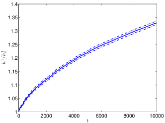
(a) $s=1$

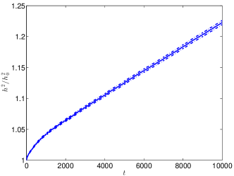
(b) $s=2$

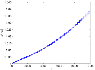
(c) $s=3$

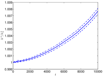
(d) $s=4$

Figure 1. Here we show ensemble averages for the evolution of normalized Sobolev norms for the initial conditions (3.1) with $\epsilon=.1$, $N=100$ and $j_{\star}=10$. The ensemble size was $10000$ and the dashed lines correspond to 95% confidence intervals.

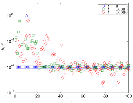
Figure 2. The evolution of a single realization from the ensemble with initial condition (3.1).

Of course, as $N\to\infty$, the nodes in (3.1) decouple. As an alternative, we consider

(3.4) $$b_{j}(\theta_{j})=\begin{cases}\frac{\epsilon}{j}\exp\left\{i\theta_{j}\right\},&j\neq j_{\star},\\ \frac{\sqrt{1-\epsilon^{2}}}{j}\exp\left\{i\theta_{j}\right\},&j=j_{\star}.\end{cases}$$

The decay in $j$ ensures that as $N\to\infty$, the solution has finite mass. The results, plotted in Figure 3, are similar to the (3.1) case. There is somewhat more growth in $h^{1}$, but less growth in the other $h^{s}$ norms.

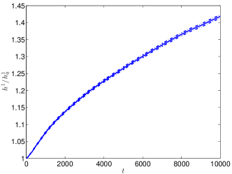
(a) $s=1$

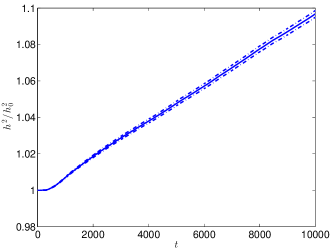
(b) $s=2$

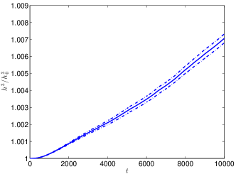
(c) $s=3$

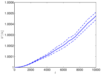
(d) $s=4$

Figure 3. Plots of normalized Sobolev norms for the initial condition (3.4) with $\epsilon=.1$, $N=100$ and $j_{\star}=10$. The ensemble size was 10000 and the dashed lines correspond to 95% confidence intervals.

4. Particular Solutions

In this section, we consider several particular solutions to (1.2), including localized solutions, periodic solutions and a “hyperbolic” solution. These were motivated by the hydrodynamic formulation of the problem, (1.8).

4.1. Localized, Uniform Phase Solutions

We first seek solutions which stay in phase for all time,

(4.1) $$\phi_{j}(t)=\phi_{j+1}(t).$$

Such solutions are said to be phase locked. Assuming this holds, (1.8) becomes

(4.2a) $$\dot{\phi}_{j} =-\rho_{j}+2\rho_{j-1}+2\rho_{j+1},$$

(4.2b) $$\dot{\rho}_{j} =0.$$

We now need a solution to

(4.3) $$-\rho_{j}+2\rho_{j-1}+2\rho_{j+1}=\omega\in\mathbb{R},\quad\text{for $j=1,\ldots N$},$$

where $\omega$ is independent of $t$ and $\rho_{0}=\rho_{N+1}=0$. This corresponds to the linear system

(4.4) $$\begin{pmatrix}-1&2&0&\cdots&0\\ 2&-1&2&\cdots&0\\ \vdots&\vdots&\ddots&\ddots&\vdots\\ 0&0&\cdots&2&-1\end{pmatrix}\boldsymbol{\rho}=\omega\boldsymbol{1}$$

Though the matrix is tri-diagonal, it is not diagonally dominant, so its solvability is not immediately clear. However,

Theorem 4.1.

The matrix in (4.4) has no kernel for any $N$.

Proof.

Letting $A_{N}$ denote this matrix, proving it has no kernel is equivalent to showing $\det A_{N}\neq 0$ for any $N$. Indeed,

(4.5) $$\begin{split}\det A_{N}&=-1\cdot\det A_{N-1}-2\cdot\begin{vmatrix}2&2&0&\cdots&0\\ 0&-1&2&\cdots&0\\ 0&2&-1&\cdots&0\\ \vdots&\ddots&\ddots&\ddots&\vdots\\ 0&0&\cdots&2&-1\end{vmatrix}\\ &=-\det A_{N-1}-4\det A_{N-2},\end{split}$$

giving us a recursion relation for the determinant. By inspection,

(4.6) $$\det A_{1}=-1,\quad\det A_{2}=-3.$$

By induction, recursion relation (4.5) demands that for all $N$, the determinant of $A_{N}$ must be odd. Hence, it is never zero. ∎

A consequence of this is the following Corollary.

Corollary 4.1.

Any nontrivial phase locked solution has $\omega\neq 0$. Moreover, given any real valued function $\omega(t)\neq 0$ for all $t\in\mathbb{R}$, there exists a nontrivial phase locked solution $\{(\phi_{j},\rho_{j})\}_{j=1}^{N}$ to (1.8).

For a given $N$, the linear system can always be solved, and a phase matched solution of (1.8) exists. However, this will not always yield a solution of (1.2). As Figure 4 shows, at $N=5$, the solution is not strictly positive, and the Madelung transformation cannot be inverted. Despite the obstacle at $N=5$, we can again obtain a strictly positive solution at $N=8$ and higher, as Figure 5 shows. It is possible to ask whether or not, there exist positive solutions for specific, but arbitrarily large, values of $N$.

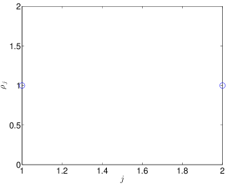
(a) $N=2$

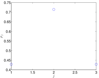
(b) $N=3$

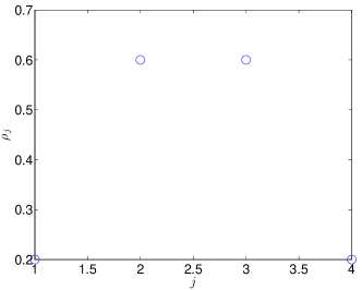
(c) $N=4$

(d) $N=5$

Figure 4. Solutions of (4.4) with $\omega=1$. The solution at $N=5$ is not strictly positive.

(a) $N=8$

(b) $N=142$

Figure 5. Solutions of (4.4) with $\omega=1$. Both solutions are strictly positive

Since the equations for the toy model, the hydrodynamic formulation and (4.4) are autonomous in $j$, one can concatenate these localized solutions together to form new solutions. For example, one could place the $N=2$ solution at lattice sites 55 and 56, and the rest to zero, within (1.2) with $N=100$. Thus, one can construct explicit solutions with isolated regions of support on arbitrarily large systems.

4.2. Time Harmonic Periodic Solutions

Here, we consider the problem with periodic boundary conditions, (1.6). Assume for all $j$ the initial condition satisfies

(4.7a) $$\rho_{j+1}(0) =\rho_{j-1}(0),$$

(4.7b) $$\phi_{j+1}(0) =\phi_{j-1}(0).$$

Furthermore, assume one or both of the variables, $\boldsymbol{\rho}$ or $\boldsymbol{\phi}$, are not uniformly constant. This will result in time harmonic solutions. This can be observed by computing

(4.8a) $$\begin{split}&\frac{d}{dt}\left(\phi_{j+1}-\phi_{j-1}\right)\\ &\quad=-\left(\rho_{j+1}-\rho_{j-1}\right)\\ &\quad\quad+2\rho_{j}\left[\cos(2(\phi_{j+1}-\phi_{j}))-\cos(2(\phi_{j}-\phi_{j-1}))\right]\\ &\quad\quad+2\rho_{j+2}\cos(2(\phi_{j+2}-\phi_{j+1}))\\ &\quad\quad-2\rho_{j-2}\cos(2(\phi_{j-1}-\phi_{j-2})),\end{split}$$

(4.8b) $$\begin{split}\frac{d}{dt}\left(\rho_{j+1}-\rho_{j-1}\right)&=4\rho_{j}\rho_{j+1}\sin(2(\phi_{j+1}-\phi_{j}))\\ &\quad-4\rho_{j+2}\rho_{j+1}\sin(2(\phi_{j+2}-\phi_{j+1}))\\ &\quad-4\rho_{j-1}\rho_{j-2}\sin(2(\phi_{j-1}-\phi_{j-2}))\\ &\quad+4\rho_{j}\rho_{j-1}\sin(2(\phi_{j}-\phi_{j-1})).\end{split}$$

If, initially, $\phi_{j+1}=\phi_{j-1}$ and $\rho_{j+1}=\rho_{j-1}$ for all $j$, then they will remain so. We also have:

• $\rho_{j}+\rho_{j-1}$ is constant in $j$ and $t$;

• $\cos(2(\phi_{j}-\phi_{j-1}))$ is constant in $j$, but may vary in $t$;

• $\sin(2(\phi_{j}-\phi_{j-1}))$ is constant in $j$, but may vary in $t$;

• $\phi_{j}+\phi_{j-1}$ is constant in $j$, but may vary in $t$.

These symmetries reduce the problem to four variables, $\rho_{j}$, $\rho_{j-1}$, $\phi_{j}$, and $\phi_{j-1}$:

(4.9a) $$\dot{\phi}_{j} =-\rho_{j}+4\rho_{j-1}\cos(2(\phi_{j}-\phi_{j-1})),$$

(4.9b) $$\dot{\phi}_{j-1} =-\rho_{j-1}+4\rho_{j}\cos(2(\phi_{j}-\phi_{j-1})),$$

(4.9c) $$\dot{\rho}_{j} =8\rho_{j}\rho_{j-1}\sin(2(\phi_{j}-\phi_{j-1})),$$

(4.9d) $$\dot{\rho}_{j-1} =-8\rho_{j}\rho_{j-1}\sin(2(\phi_{j}-\phi_{j-1})).$$

Defining

(4.10a) $$\bar{\phi} \equiv\phi_{j}+\phi_{j-1},$$

(4.10b) $$\Delta\phi \equiv\phi_{j}-\phi_{j-1},$$

(4.10c) $$\bar{\rho} \equiv\rho_{j}+\rho_{j-1},$$

(4.10d) $$\Delta{\rho} \equiv\rho_{j}-\rho_{j-1},$$

we have:

(4.11a) $$\frac{d}{dt}{\bar{\phi}} =-{\bar{\rho}}+4\bar{\rho}\cos(2\Delta\phi),$$

(4.11b) $$\frac{d}{dt}{\Delta\phi} =-{\Delta\rho}-4\Delta{\rho}\cos(2\Delta\phi),$$

(4.11c) $$\frac{d}{dt}{\bar{\rho}} =0,$$

(4.11d) $$\frac{d}{dt}{\Delta\rho} =16\rho_{j}\rho_{j-1}\sin(2\Delta\phi).$$

Since $\bar{\rho}^{2}-\Delta\rho^{2}=4\rho_{j}\rho_{j-1}$ and $\bar{\rho}$ is invariant, we have a closed system of $2$ equations for $\Delta\phi$ and $\Delta\rho$.

(4.12a) $$\frac{d}{dt}{\Delta\phi} =-{\Delta\rho}\left[1+4\cos(2\Delta\phi)\right],$$

(4.12b) $$\frac{d}{dt}{\Delta\rho} =4\left(\bar{\rho}^{2}-\Delta\rho^{2}\right)\sin(2\Delta\phi).$$

The system is Hamiltonian with

(4.13) $$H=\frac{1}{2}\left(1+4\cos(2\Delta\phi)\right)\left(\bar{\rho}^{2}-\Delta\rho^{2}\right)$$

and symplectic structure

(4.14) $$\frac{d}{dt}\Delta\phi=\frac{\partial H}{\partial\Delta\rho},\quad\frac{d}{dt}\Delta\rho=-\frac{\partial H}{\partial\Delta\phi}.$$

Thus, we anticipate time harmonic motion. An example appears in Figure 6, where the initial condition is

(4.15a) $$\rho_{1}=\rho_{2}=1,$$

(4.15b) $$\phi_{1}=\frac{\pi}{4},\quad\phi_{2}=0.$$

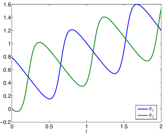
Figure 6.

5. Discrete Rarefaction Waves and Weak Turbulence

In this section, we explore the dynamics when the initial configuration is given by the out of phase initial condition $\phi_{j}=\phi_{j+1}-\frac{\pi}{4}$. If this phase relation were to somehow persist, the resulting equations hints at the discrete Burger’s formulation of the hydrodynamic equations

(5.3) $$\left\{\begin{array}[]{l}\dot{\phi}_{j}=0,\\ \dot{\rho}_{j}=-4\rho_{j}\rho_{j-1}+4\rho_{j}\rho_{j+1}=-8\rho_{j}\left(\frac{\rho_{j+1}-\rho_{j-1}}{2}\right).\end{array}\right.$$

This has discrete rarefaction and shock wave dynamics. We call (5.3) the discrete Burger’s equation since, were we to discretize

$$\rho_{t}=-8\rho\nabla\rho,$$

in space and take the gridpoint spacing paramter equal to one, we would recover the above equation. We note here that the rarefaction waves we observe have similar dynamics to those found in Fermi-Pasta-Ulam chains, see [8].

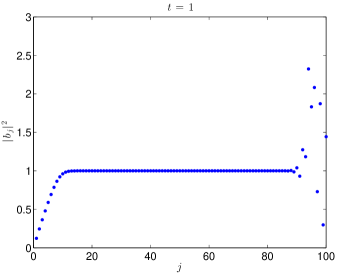
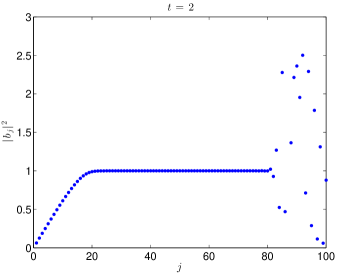
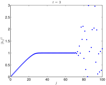
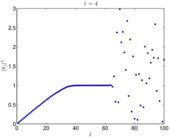
Figure 7. A combination of discrete rarefaction and dispersive shocking. As an initial condition, $\rho_{j}=1$ at all values of $j$.

However in (1.8), there are additional terms which prevent this phase relation from persisting. We show here how the solutions evolve, with the initial condition

(5.4) $$b_{j}=\exp i\left\{(j-1)\pi/4\right\}.$$

As a first example, we solve (1.2) with the initial condition (5.4) over $N=100$ lattice sites. The results appear in Figures 7 and 8. As can be seen, the $h^{s}$ norms eventually cease to be monotonic. To see persistent growth in the norms, we can look at a system with $N=5000$ sites and for longer a time; see Figures 9 and 10.

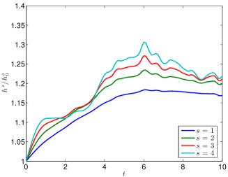
Figure 8. Growth in the $h^{s}$ norms for the dynamics of Figure 7.

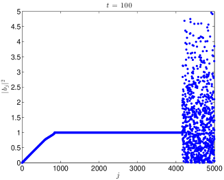
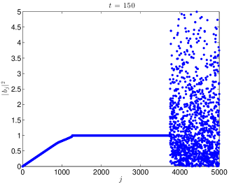
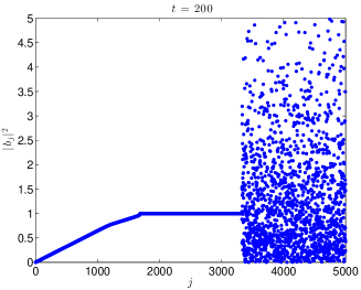
Figure 9. A combination of discrete rarefaction and dispersive shocking. As an initial condition, $\rho_{j}=1$ at all values of $j$.

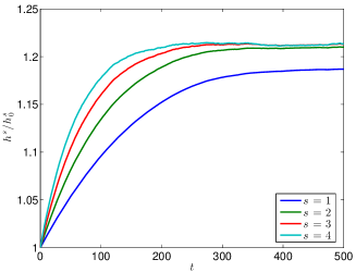
Figure 10. Growth in the $h^{s}$ norms for the dynamics of Figure 9.

The simulation on $N=5000$ reveals that the rarefaction portion of the solution has more structure than is apparent in the case of $N=100$. As shown in Figure 11, the rarefaction wave evolves with several different slopes.

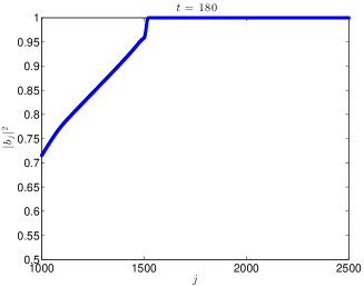
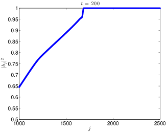
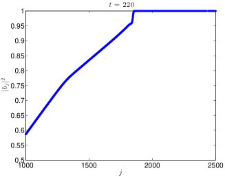
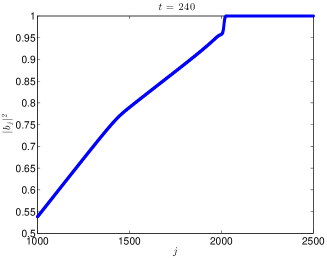
Figure 11. A close up of the front for the discrete rarefaction wave. As an initial condition, $\rho_{j}=1$ at all values of $j$.

Unfortunately, as $N\to\infty$, (5.4) will not correspond to a finite mass solution. Thus, we studied the weighted initial condition,

(5.5) $$b_{j}=\exp i\left\{(j-1)\pi/4\right\}/j.$$

This, too, results in energy transfer, though it is not monotonic. Several frames from this simulation appear in Figure 12, and the growth of the norms can be seen in Figure 13. The norm growth is quite pronounced; this may be due to an inability of mass to propagate backwards, against the weight $1/j$.

In similar calculations with

(5.6) $$b_{j}=\exp i\left\{(j-1)\pi/4\right\}/{(w(j))^{\sigma}}.$$

for $0<\sigma<1$, where $w(j)\to\infty$ as $j\to\infty$, we observe that some form of the rarefaction front propagates forward even with a tail in the higher nodes and that the structure of the rarefaction wave persists longer as $\sigma\to 0$. Since the rarefaction wave and the backward dispersive shock travel at finite speeds in the simulation, we observe motion to large $j$ on much longer time scales for large $N$. Here, the weights in (5.6) allow us to study rarefaction waves in a setting with $h^{1}$ norms of order $1$ instead of order $N$. In addition, we observe that the rarefaction wave solution is robust even for initial data of the form (5.6), which has less back scattering thanks to the smaller jump at the right endpoint. As the rarefaction front enters the decaying tail, it does however begin to lose some mass at regular intervals, but continues to propagate weakly.

All rarefaction wave solutions presented in this section result in norm growth when mapped back to solutions of (1.1). This is due to Proposition $2.1$ of [4], which states that a mass shift to the higher nodes in the Toy Model results in growth of higher Sobolev norms of the corresponding solution to (1.1). This is fundamental to showing the importance of tracking the rarefaction wave front moving toward large $j$ in (1.2). However, a more detailed result relating to the frequency scales at each generation $\Lambda_{j}$ and a better categorization of families of resonant frequencies would be required to address this issue in its entirety and observe a rarefaction front in the resonant frequencies of the torus. It is unclear at this point how to directly translate solutions with frequency cascades in (1.2) to computationally observable solutions with frequency cascades leading to $H^{s}$ norm growth for $s>1$ in (1.1). Here, however, we have demonstrated the robustness of solutions that move mass in (1.2) from low to high $j$.

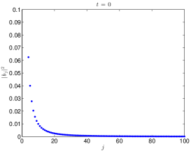
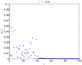
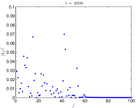
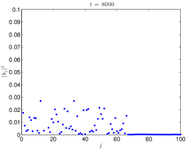
Figure 12. Evolution of the initial condition (5.5).

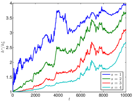
Figure 13. Growth in the $h^{s}$ norms for the dynamics of Figure 12.

6. Continuum Limit & Compacton Type Solutions

As a final observation, let us introduce the parameter $0<h\ll 1$, such that

(6.1) $$B(x_{j},t)=b_{j}(t),\quad x_{j}=hj.$$

Taylor expanding,

(6.2) $$-i\partial_{t}B=\left[3B^{2}+4h^{2}\left((\partial_{x}B)^{2}+B\partial_{x}^{2}B\right)+\mathrm{O}(h^{4})\right]\overline{B}.$$

Neglecting $\mathrm{O}(h^{4})$ terms,

(6.3) $$-i\partial_{t}B=3\lvert B\rvert^{2}B+4h^{2}\overline{B}\partial_{x}\left(B\partial_{x}B\right).$$

This retains the toy model scaling that if $B(x,t)$ is a solution, then so is $\lambda B(x,\lambda^{2}t)$. It is also invariant to multiplication by an arbitrary phase.

The equation (6.3) is, formally, degenerately dispersive, and it can be viewed as an NLS analog of the compacton equations, [13, 10, 11, 12]. One of the interesting features of the compacton equations is that they admit compactly supported nonlinear bound states, which we now seek for (6.3). We begin with the ansatz $B=e^{it}Q(x)$, $Q>0$. Consequently, $Q$ solves

(6.4) $$Q=3Q^{3}+4h^{2}Q(QQ^{\prime})^{\prime}$$

which can be expressed as

(6.5) $$Q=3Q^{3}+2h^{2}Q(Q^{2})^{\prime\prime}$$

Letting $U=Q^{2}$,

(6.6) $$2h^{2}U^{\prime\prime}+3U-1=0$$

This can be integrated up once to

(6.7) $$h^{2}U^{\prime 2}+{\frac{3}{2}U^{2}-U}=C$$

$h$ can easily be scaled out by changing the dependent variable, thus we set $h=1$. We always have a potential well in this equation, so there should be homoclinic orbits.

If $C=0$, then $0<U<2/3$. The explicit solution is

(6.8) $$Q(x)=\sqrt{\frac{2}{3}}\sin\left(\frac{1}{2}\sqrt{\frac{3}{2}}x\right).$$

Putting $h$ in,

(6.9) $$Q_{h}(x)=\sqrt{\frac{2}{3}}\sin\left(h^{-1}\frac{1}{2}\sqrt{\frac{3}{2}}x\right).$$

Phase shifting the solution by $\pi/2$, we can alternatively have

(6.10) $$Q_{h}(x)=\sqrt{\frac{2}{3}}\cos\left(h^{-1}\frac{1}{2}\sqrt{\frac{3}{2}}x\right).$$

We can turn this into a compact structure if we now define

(6.11) $$Q_{h}^{c}(x)=\begin{cases}\sqrt{\frac{2}{3}}\cos\left(h^{-1}\frac{1}{2}\sqrt{\frac{3}{2}}x\right)&\lvert x\rvert<h\pi\sqrt{\frac{2}{3}}\\ 0&\lvert x\rvert\geq h\pi\sqrt{\frac{2}{3}}.\end{cases}$$

This structure, with $h=1$, appears in Figure 14.

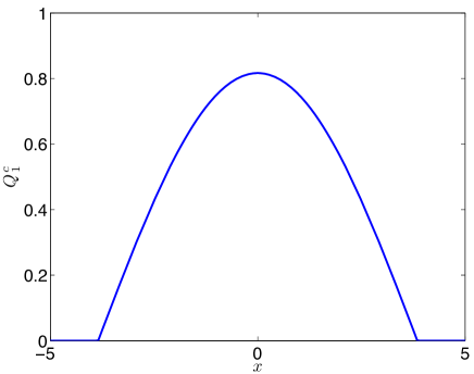
Figure 14. The compacton solution given by (6.11).

Note that this will satisfy the equation in the strong sense. If we go back to the sine formulation and look at $x=0$ with $h=1$, then

$$Q^{c}(x)=\begin{cases}\sqrt{\frac{2}{3}}\sin\left(\frac{1}{2}\sqrt{\frac{3}{2}}x\right)&0<x<\pi\sqrt{\frac{2}{3}}\\ 0&\textrm{otherwise}.\end{cases}$$

Then, near $x=0$,

(6.12a) $$Q^{c}(x) \sim xH(x)$$

(6.12b) $$(Q^{c}(x))^{2} \sim x^{2}H(x)$$

(6.12c) $$\frac{d^{2}}{dx^{2}}(Q^{c}(x))^{2} \sim H(x)$$

(6.12d) $$Q^{c}(x)\frac{d^{2}}{dx^{2}}(Q^{c}(x))^{2} \sim xH(x),$$

where $H(x)$ is the Heaviside function. Hence, the most degenerate term in (6.5) is continuous.

References

• [1] V. Arnold. Instability of dynamical systems with many degrees of freedom. Dokl. Akad. Nauk SSSR, 146:9–12, 1964.
• [2] J. Bourgain. Remarks on stability and diffusion in high-dimensional hamiltonian systems and partial differential equations. Ergodic Theory Dynam. Systems, 24(5):1331–1357, June 2004.
• [3] R. Carles and E. Faou. Energy cascades for NLS on the torus. Discrete and Continuous Dynamical Systems. Series A, 32(6):2063–2077, June 2012.
• [4] J. Colliander, M. Keel, G. Staffilani, H. Takaoka, and T. Tao. Transfer of energy to high frequencies in the cubic defocusing nonlinear Schrödinger equation. Inv. Math., 181(1):39–113, 2012.
• [5] M. Galassi et al. GNU Scientific Library Reference Manual (3rd Ed.). Network Theory Ltd., 2009.
• [6] M. Guardia and V. Kaloshin. Growth of sobolev norms in the cubic defocusing nonlinear schrödinger equation. preprint, 2012.
• [7] Z. Hani. Global and dynamical aspects of nonlinear Schrödinger equations on compact manifolds. Doctoral Dissertation - UCLA, 2011.
• [8] M. Herrmann and J. D. M. Rademacher. Riemann solvers and undercompressive shocks of convex fpu chains. Nonlinearity, 23:277–303, 2010.
• [9] S. B. Kuksin. Oscillations in space-periodic nonlinear schrödinger equations. Geom. Func. Anal., 7(2):338–363, 1997.
• [10] P. S. Rosenau. Nonlinear dispersion and compact structures. Physical Review Letters, 73(13):1737–1741, 1994.
• [11] P. S. Rosenau. What is $\dots$ a compacton? Notices of the American Mathematical Society, 52(7):738–739, 2005.
• [12] P. S. Rosenau. Compact breathers in a quasi-linear Klein-Gordon equation. Physics Letters, Section A: General, Atomic and Solid State Physics, 374(15-16):1663–1667, 2010.
• [13] P. S. Rosenau and J. M. Hyman. Compactons: Solitons with finite wavelength. Physical Review Letters, 70(5):564–567, 1993.
• [14] P. E. Zhidkov. Korteweg-de Vries and nonlinear Schrödinger equations: qualitative theory. Springer Lecture Notes in Mathematics, $1756$, 2001.