Increasing sync rate of pulse-coupled oscillators via phase response function design: theory and application to wireless networks

Abstract

This paper addresses the synchronization rate of weakly connected pulse-coupled oscillators (PCOs). We prove that besides coupling strength, the phase response function is also a determinant of synchronization rate. Inspired by the result, we propose to increase the synchronization rate of PCOs by designing the phase response function. This has important significance in PCO-based clock synchronization of wireless networks. By designing the phase response function, synchronization rate is increased even under a fixed transmission power. Given that energy consumption in synchronization is determined by the product of synchronization time and transformation power, the new strategy reduces energy consumption in clock synchronization. QualNet experiments confirm the theoretical results.

I Introduction

In recent years, synchronization of oscillating dynamical systems is receiving increased attention. One particular class of oscillating dynamical systems, pulse-coupled oscillators (PCOs), are of considerable interest. ‘Pulse-coupled’ means that oscillators interact with each other using pulse-based communication, i.e., they can achieve synchronization via the exchange of simple identical pulses. PCO has been used to describe many biological synchronization phenomena such as the flashing of fireflies, the contraction of cardiac cells, and the firing of neurons [1]. Recently, with the progress of ultra-wide bandwidth (UWB) impulse radio technology [2], the PCO based synchronization scheme has also been applied to synchronize wireless networks [3, 4, 5, 6, 7]. Since it is implemented at the physical layer or MAC (Media Access Control) layer, it eliminates the high-layer intervention. Moreover, message exchanging in PCO-based synchronization strategy is independent of the origin of the pulses, which avoids requiring memory to store time information of other nodes [3]. Therefore, the PCO-based synchronization scheme has received increased attention in the communication community recently.

Despite considerable work on synchronization conditions, there remains a lack of research on the synchronization rate for PCOs, especially for PCOs with a general coupling structure other than the commonly studied all-to-all structure. The synchronization rate is crucial in synchronization processes [8]. For example, in the clock synchronization of wireless networks, the synchronization rate is a determinant of the consumption in energy, which is a precious system resource [3].

This paper analyzes the synchronization rate of weakly connected PCOs in the presence of combined global cues (also called leader, or pinner in the language of pinning control [9]) and local cues (alternatively, local coupling). The network structure is considered because in the clock synchronization of wireless networks, usually different time references are synchronized through internal interplay between different nodes and external coordination from a global time base such as GPS [10]. Due to pulsatile coupling, the synchronization rate of PCOs are very difficult to study analytically [1]. Based on the assumption of ‘weakly connected’, we study the problem using phase response functions. A phase response function describes the phase correction of an oscillator induced by a pulse from neighboring oscillators or external stimuli [11]. Under the assumption of weak coupling, we transform the PCO model into a simpler phase model, based on which we analyze the synchronization rate of PCOs. In fact, we will prove that the synchronization rate is determined not only by the strength of global and local cues, but also by the phase response function. This means that different phase response functions bring different synchronization rates even when the coupling strength is fixed. This has great significance for synchronization strategies such as the clock synchronization of wireless networks, where the phase response function is a design parameter. By designing the phase response function, we increase the synchronization rate under a fixed coupling strength. Given that the total energy consumption in synchronization is determined by the product of synchronization time and transmission power (corresponding to coupling strength and topology) [3, 12], the new strategy reduces energy consumption in synchronization in that synchronization time is reduced under a fixed transmission power. It is worth noting that the assumption of weak coupling is well justified by biological observations: the amplitudes of postsynaptic potentials are around 0.1 mV, which is small compared with the amplitude of excitatory postsynaptic potential necessary to discharge a quiescent cell (around 20 mV) [13]. In PCO-based wireless network synchronization schemes, weak coupling is also necessary to guarantee a robust synchronization [3].

II Problem formulation and Model transformations

Consider a network of $N$ pulse-coupled oscillators, which will henceforth be referred to as ‘nodes’. All oscillator nodes or a portion of them can receive alignment/entrainment information from an external global cue (also called leader, or pinner in the language of pinning control [9]).

We denote the dynamics of the oscillator network as

$$\dot{x}_{g} =f_{g}(x_{g})$$ (1)

$$\dot{x}_{i} =f_{i}(x_{i})+g_{i}\delta(t-t_{g})+l\sum_{1\leq j\leq N,\,j\neq i}a_{i,j}\delta(t-t_{j})$$

for $i=1,2,\ldots,N$, where $x_{g}\in[0,\,1]$ and $x_{i}\in[0,\,1]$ denote the states of the global cue and oscillator nodes, respectively. $f_{g}$ and $f_{i}$ describe their dynamics. $g_{i}\geq 0$ denotes the effect of the global cue’s firing on oscillators $i$: when $x_{g}$ reaches 1 (at time instant $t_{g}$), it fires and returns to 0, and at the same time increases oscillator $i$ by an amount $g_{i}$. $l\geq 0$ and $a_{ij}\in\{0,\,1\}$ denote the effect of oscillator $j$’s firing on oscillator $i$: when $x_{j}$ reaches 1 (at time instant $t_{j}$), it fires and resets to 0, and at the same time pulls oscillator $i$ up by an amount $la_{i,j}$. The increased amount is produced by dirac function $\delta(t)$, which is zero for all $t$ except $t=0$ and satisfies $\int_{-\infty}^{\infty}\delta(t)dt=1$.

Remark 1

If $g_{i}$ (or $a_{i,j}$) is $0$, then oscillator $i$ is not affected by the global cue (or oscillator $j$).

Assumption 1

We assume $a_{i,j}=a_{j,i}$, which is common in wireless networks [14, 15].

Assumption 2

We assume weak coupling [13], i.e., $g$ and $l$ satisfy $g\ll 1$ and $l\ll 1$.

Assumption 2 follows from the fact that the amplitudes of postsynaptic potentials measured in the soma of neurons are far below the amplitude of the mean excitatory postsynaptic potential necessary to discharge a quiescent cell [13], it is also required in PCO-based wireless network synchronization strategies to ensure the robustness of synchronization [3].

Based on Assumption 2, the system in (1) can be described by the following phase model using the classical phase reduction technique and phase averaging technique [11, 16]:

$$\dot{\theta}_{g} =w_{g}$$ (2)

$$\dot{\theta}_{i} =w_{i}+\frac{g_{i}}{T}Q_{g}(\theta_{g}-\theta_{i})+\frac{l}{T}\sum_{1\leq j\leq N,j\neq i}a_{i,j}Q_{l}(\theta_{j}-\theta_{i})$$

for $i=1,2,\ldots,N$, where $\theta_{g}\in[0,\,2\pi)$ and $\theta_{i}\in[0,\,2\pi)$ denote the phases of the global cue and oscillator $i$, respectively. $Q_{g}(x)$ and $Q_{l}(x)$ are phase response functions and are often referred to as phase response curves in biological study. They are periodic functions with period $2\pi$ [11, 16]. $T$ is the period of the global cue. $w_{g}$ and $w_{i}$ denote the natural frequencies of the global cue and oscillator $i$, respectively.

Remark 2

The transformation from (1) to (2) is a standard practice in the study of weakly connected PCOs and it is applicable to any limit-cycle oscillation function $f_{i}$ and $f_{g}$ [11]. The detailed procedure has been well documented in [16], Chapter 9 of [13], and Chapter 10 of [11].

Assumption 3

In the paper, we assume that $Q_{p}\,(p=\{l,\,g\})$ satisfy the following conditions:

$$Q_{p}(0)=0;\>\forall x\in(-\pi,\pi),\frac{Q_{p}(x)}{x}>0;Q_{p}(-x)=-Q_{p}(x)$$ (3)

Remark 3

Assumption 3 gives an advance-delay phase response function, which is common in biological oscillators [11]. Moreover, given that in wireless networks, the phase response function is a design parameter, Assumption 3 will simplify analysis and design, and as shown later, such phase response functions will also lead to good synchronization properties.

Solving the first equation in (2) gives the dynamics of the global cue $\theta_{g}=w_{g}t+\xi_{g}$, where the constant $\xi_{g}$ denotes the initial phase of the global cue. To study if local oscillators can be synchronized to the global cue, it is convenient to study the phase deviation of local oscillators from the global cue. So we introduce the following change of variables:

$$\theta_{i}=\theta_{g}+\xi_{i}=w_{g}t+\xi_{g}+\xi_{i}$$ (4)

Therefore $\xi_{i}\in[-\pi,\,\pi]$ denotes the phase deviation of the $i$th oscillator from the global cue. Substituting (4) into (2) yields the dynamics of phase deviations $\xi_{i}$:

$$\dot{\xi}_{i}=\Delta_{i}-\frac{g_{i}}{T}Q_{g}(\xi_{i})+\frac{l}{T}\sum_{1\leq j\leq N,j\neq i}a_{i,j}Q_{l}(\xi_{j}-\xi_{i})$$ (5)

for $i=1,2,\ldots,N$, where $\Delta_{i}=w_{i}-w_{g}$. In (5), the oddness property of function $Q_{g}$ is exploited.

Assumption 4

In this paper, we assume $w_{i}=w_{g}$ is satisfied for all $i=1,2,\ldots,N$, i.e., all the oscillators have the same natural frequency as the global cue.

Using Assumption 4, (5) reduces to:

$$\dot{\xi}_{i}=-\frac{g_{i}}{T}Q_{g}(\xi_{i})+\frac{l}{T}\sum_{1\leq j\leq N,j\neq i}a_{i,j}Q_{l}(\xi_{j}-\xi_{i})$$ (6)

for $i=1,2,\ldots,N$.

Thus far, by analyzing the properties of (6), we can obtain the roles of global and local cues as well as phase response functions in the synchronization of PCO networks:

• Synchronization: If all $\xi_{i}$ asymptotically converge to $0$, then we have $\theta_{1}=\theta_{2}=\ldots=\theta_{N}$ when time goes to infinity, meaning that all the nodes are synchronized to the global cue.

• Exponential bound on the synchronization rate: From dynamic systems theory [17], the synchronization rate is determined by the rate at which $\xi_{i}$ decays to $0$, namely, it can be measured by the maximal value of $\alpha$ $(\alpha>0)$ satisfying the following inequality for some constant $C$:

  $$\|\xi(t)\|\leq Ce^{-\alpha t}\|\xi(0)\|,\quad\xi=\left[\begin{array}[]{cccc}\xi_{1}&\xi_{2}&\ldots&\xi_{N}\end{array}\right]^{T}$$ (7)

  where $\|\bullet\|$ is the Euclidean norm. A larger $\alpha$ leads to a faster synchronization rate.

Assigning arbitrary orientation to each interaction, we can get the $N\times M$ incidence matrix $B$ ($M$ is the number of non-zero $a_{i,j}\,(1\leq i\leq N,\,j<i)$, i.e., the number of interaction edges) of the interaction [18]: $B_{i,j}=1$ if edge $j$ enters node $i$, $B_{i,j}=-1$ if edge $j$ leaves node $i$, and $B_{i,j}=0$ otherwise. Then using graph theory, we can write (6) in a more compact matrix form:

$$\dot{\xi}=-\frac{1}{T}GQ_{g}(\xi)-\frac{l}{T}BQ_{l}\left(B^{T}\xi\right)$$ (8)

where $\xi$ is given in (7), $G=\textrm{diag}\left\{g_{1},\>g_{2},\>\ldots,\>g_{N}\right\}$, and $\textrm{diag}\{\bullet\}$ denotes a diagonal matrix with elements $\{\bullet\}$ on the diagonal.

III Synchronization of Pulse Coupled Oscillators

III-A When all $\xi_{i}$ are within $(-\frac{\pi}{2},\,\frac{\pi}{2})$

Theorem 1

For the oscillator network in (8), if all $\xi_{i}$ are within $[-\varepsilon,\,\varepsilon]$ for some $\varepsilon\in[0,\,\frac{\pi}{2})$, then the network synchronizes to the global cue when at least one $g_{i}$ is positive and the local coupling topology $a_{i,j}$ is connected. Here ‘connected’ means that there is a multi-hop path (i.e., a sequence with nonzero values $a_{i,m_{1}}$, $a_{m_{1},m_{2}}$, $\ldots,$ $a_{m_{p-1},m_{p}}$, $a_{m_{p},j}$) from each node $i$ to every other node $j$.

Proof:

We first prove that for any $0\leq\varepsilon<\frac{\pi}{2}$, when $\xi\in[-\varepsilon,\,\varepsilon]\times\ldots\times[-\varepsilon,\,\varepsilon]\triangleq[-\varepsilon,\,\varepsilon]^{N}$ where $\times$ is Cartesian product, they will remain in the interval, i.e, $[-\varepsilon,\,\varepsilon]^{N}$ is positively invariant for (8). To this end, we only need to check the direction of the vector field on the boundaries. If $\xi_{i}=\varepsilon$, we have $0\leq\xi_{i}-\xi_{j}\leq 2\varepsilon<\pi$ for $1\leq j\leq N$, so from (6) and the properties of phase response functions in Assumption 3, $\dot{\xi}_{i}<0$ holds. Hence the vector field is pointing inward in the set, and no trajectories can escape to values larger than $\varepsilon$. Similarly, we can prove that when $\xi_{i}=-\varepsilon$, $\dot{\xi}_{i}>0$ holds. Thus the vector field is pointing inward in the set, and no trajectories can escape to values smaller than $-\varepsilon$. Therefore $[-\varepsilon,\,\varepsilon]^{N}$ is positively invariant for any $0\leq\varepsilon<\frac{\pi}{2}$.

Next we proceed to prove synchronization. Construct a Lyapunov function as $V=\frac{1}{2}\xi^{T}\xi$. $V$ is non-negative and will be zero if and only if all $\xi_{i}$ are zero, meaning that all oscillators are synchronized to the global cue.

Differentiating $V$ along the trajectories of (8) yields

$$\dot{V}=\xi^{T}\dot{\xi} =-\frac{1}{T}\xi^{T}GS_{1}\xi-\frac{l}{T}\xi^{T}BS_{2}B^{T}\xi$$ (9)

$$=-\frac{1}{T}\xi^{T}\left(GS_{1}+lBS_{2}B^{T}\right)\xi$$

where $S_{1}$ and $S_{2}$ are given by

$$S_{1}=\textrm{diag}\left\{\frac{Q_{g}(\xi_{1})}{\xi_{1}},\,\frac{Q_{g}(\xi_{2})}{\xi_{2}},\,\ldots,\,\frac{Q_{g}(\xi_{N})}{\xi_{N}}\right\},$$ (10)

$$S_{2}=\textrm{diag}\left\{\frac{Q_{l}((B^{T}\xi)_{1})}{(B^{T}\xi)_{1}},\,\frac{Q_{l}((B^{T}\xi)_{2})}{(B^{T}\xi)_{2}},\,\ldots,\,\frac{Q_{l}((B^{T}\xi)_{M})}{(B^{T}\xi)_{M}}\right\}$$ (11)

with $(B^{T}\xi)_{i}\,(1\leq i\leq M)$ denoting the $i$th element of the $M\times 1$ dimensional vector $B^{T}\xi$.

According to dynamic systems theory [17], if $GS_{1}+lBS_{2}B^{T}$ in (9) is positive definite, then $\dot{V}$ is always negative when $\xi\neq 0$ and $V$ will decay to zero exponentially, meaning that $\xi$ will converge to zero and all oscillators are synchronized to the global cue.

Note that $(B^{T}\xi)_{i}\,(1\leq i\leq M)$ are in the form of $\xi_{m}-\xi_{n}\,(1\leq m,n\leq N)$, it follows that $(B^{T}\xi)_{i}$ are restricted to $[-2\varepsilon,\,2\varepsilon]$ when all $\xi_{j}$ are in $[-\varepsilon,\,\varepsilon]$ for some $\varepsilon\in[0,\,\frac{\pi}{2})$. Given that in $(-\pi,\,\pi)$, $Q_{g}(x)$ and $Q_{l}(x)$ satisfy $\frac{Q_{g}(x)}{x}>0,\>\frac{Q_{l}(x)}{x}>0$, it follows that $S_{1}$ and $S_{2}$ are positive definite, and thus the following inequalities are satisfied for some positive constants $\sigma_{1}$ and $\sigma_{2}$:

$$S_{1}\geq\sigma_{1}I,\quad S_{2}\geq\sigma_{2}I,$$ (12)

$$\sigma_{1}=\min\limits_{-\varepsilon\leq x\leq\varepsilon}\frac{Q_{g}(x)}{x},\quad\sigma_{2}=\min\limits_{-2\varepsilon\leq x\leq 2\varepsilon}\frac{Q_{l}(x)}{x},\quad\varepsilon\in[0,\,\frac{\pi}{2})$$

So we have $GS_{1}+lBS_{2}B^{T}\geq\sigma_{1}G+\sigma_{2}lBB^{T}$, which in combination with (9) produces

$$\dot{V}\leq-\frac{1}{T}\xi^{T}\left(\sigma_{1}G+\sigma_{2}lBB^{T}\right)\xi$$ (13)

Next we prove that $\sigma_{1}G+\sigma_{2}lBB^{T}$ is positive definite, which leads to $\dot{V}<0$ for $\xi\neq 0$.

It can be easily verified that $\sigma_{1}G+\sigma_{2}lBB^{T}$ is of the following form:

$$\sigma_{1}G+\sigma_{2}lBB^{T}=\sigma_{1}{\rm diag}\{g_{1},\,g_{2},\,\ldots,\,g_{N}\}+\sigma_{2}lL$$ (14)

with $L\in\mathcal{R}^{N\times N}$ constructed as follows: for $i\neq j$, its $(i,j)$th element is $-a_{i,j}$, for $i=j$, its $(i,j)$th element is $\sum\limits_{m=1,m\neq i}^{N}a_{i,m}$. Since $\sigma_{1}$, $\sigma_{2}$, and $l$ are positive, and $g_{i}$, $a_{i,j}$ are non-negative, it follows from the Gershgorin Circle Theorem that $\sigma_{1}G+\sigma_{2}lBB^{T}$ only has non-negative eigenvalues [19]. Next we prove its positive definiteness by excluding $0$ as an eigenvalue.

Since the topology of local coupling $a_{i,j}$ is connected, $\sigma_{1}G+\sigma_{2}lBB^{T}$ is irreducible according to graph theory [19]. This in combination with the assumption of at least one non-zero $g_{i}$ guarantees that $\sigma_{1}G+\sigma_{2}lBB^{T}$ is irreducibly diagonally dominant. So from Corollary 6.2.27 of [19], we know the determinant of $\sigma_{1}G+\sigma_{2}lBB^{T}$ is non-zero and hence 0 is not its eigenvalue. Therefore $\sigma_{1}G+\sigma_{2}lBB^{T}$ is positive definite, and $V$ will converge to $0$. ∎

III-B When all $\xi_{i}$ are within $(-\pi,\,\pi)$ and the maximal/minimal $\xi_{i}$ is outside $(-\frac{\pi}{2},\,\frac{\pi}{2})$

Theorem 2

For the oscillator network in (8), if all $\xi_{i}$ are within $[-\varepsilon,\varepsilon]$ for some $\varepsilon\in[\frac{\pi}{2},\,\pi)$ and the maximal/minimal $\xi_{i}$ is outside $(-\frac{\pi}{2},\,\frac{\pi}{2})$, then the oscillator network will synchronize to the global cue when all nodes are connected to the global cue, and the following relations are satisfied:

$$g_{\min}>\frac{\sigma_{4}l\lambda_{\max}(BB^{T})}{\sigma_{3}},$$ (15)

$$g_{i}\geq\frac{l}{\gamma_{1}}\sum_{1\leq j\leq N,j\neq i}a_{i,j}\gamma_{2},\quad i=1,2,\ldots,N$$

where $\lambda_{\max}$ denotes the maximal eigenvalue, $g_{\min}=\min\{g_{1},\,g_{2},\,\ldots,\,g_{N}\}$, and

$$\sigma_{3}=\min\limits_{-\varepsilon\leq x\leq\varepsilon}\frac{Q_{g}(x)}{x},\,\sigma_{4}=\max\limits_{-2\varepsilon\leq x\leq 2\varepsilon}\frac{-Q_{l}(x)}{x},$$ (16)

$$\gamma_{1}=\min\limits_{0\leq x\leq\varepsilon}Q_{g}(x),\,\gamma_{2}=\max\limits_{0\leq x\leq 2\varepsilon}-Q_{l}(x),\,\varepsilon\in[\frac{\pi}{2},\,\pi)$$

Proof:

Following the line of reasoning of Theorem 1, we can prove that if the second inequality in (15) holds, then for any $\frac{\pi}{2}\leq\varepsilon<\pi$, $[-\varepsilon,\,\varepsilon]^{N}$ is positively invariant for (8), i.e., for $\xi\in[-\varepsilon,\,\varepsilon]^{N}$, it will always remain in the interval. Next we proceed to prove synchronization.

Choose the same Lyapunov function $V$ as the proof of Theorem 1. Then we have

$$\dot{V}=\xi^{T}\dot{\xi} =-\frac{1}{T}\xi^{T}GS_{1}\xi-\frac{l}{T}\xi^{T}BS_{2}B^{T}\xi$$ (17)

$$=-\frac{1}{T}\xi^{T}\left(GS_{1}+lBS_{2}B^{T}\right)\xi$$

where $S_{1}$ and $S_{2}$ are given in (10) and (11), respectively.

When the maximal/minimal $\xi_{i}$ is outside $(-\frac{\pi}{2},\,\frac{\pi}{2})$, $\xi_{m}-\xi_{n}\,(1\leq m,n\leq N)$ may be outside $(-\pi,\,\pi)$. So in (10) and (11), the domain of $Q_{g}(x)$ is within $(-\pi,\,\pi)$, on which $Q_{g}(x)$ satisfies $Q_{g}(x)/x>0$, and the domain of $Q_{l}(x)$ is not restricted to $(-\pi,\,\pi)$, outside of which, $Q_{l}(x)/x$ may be positive or negative. Therefore $S_{1}$ is still positive definite, but $S_{2}$ may be positive definite, negative definite or indefinite. From the definition of $\sigma_{3}$ and $\sigma_{4}$ in (16), we have:

$$GS_{1}\geq\sigma_{3}g_{\min},\quad-lBS_{2}B^{T}\leq\sigma_{4}l\lambda_{\max}(BB^{T})$$

Notice that $Q_{l}(x)$ is periodic with period $2\pi$, and $\frac{Q_{l}(x)}{x}>0$ holds for all $-\pi<x<\pi$, we know for any $\frac{\pi}{2}\leq\varepsilon<\pi$, if $x_{0}\in[-2\varepsilon,\,-\pi]$, then $Q_{l}(x_{0})=Q_{l}(2\pi+x_{0})\geq 0$ holds since $2\pi+x_{0}$ resides in the interval $[2(\pi-\varepsilon),\,\pi]$. Thus it follows $\frac{Q_{l}(x_{0})}{x_{0}}=\frac{Q_{l}(x_{0}+2\pi)}{x_{0}}\leq 0$, which means $\sigma_{4}\geq 0$.

Therefore, (15) guarantees the positive definiteness of $GS_{1}+lBS_{2}B^{T}$, and hence the synchronization of the oscillators to the global cue. ∎

Remark 4

Theorem 2 indicates that when the maximal/minimal phase difference is outside $(-\frac{\pi}{2},\,\frac{\pi}{2})$, all oscillators have to connect to the global cue to ensure synchronization to the global cue. This is consistent with existing results which have shown that for some initial conditions (even with measure zero), PCOs cannot be synchronized by local coupling [1]. In fact, most of the existing results on PCOs are based on all-to-all connection, which amounts to $g_{\min}>0$.

Remark 5

Theorem 2 reveals that a strong local cue does not necessarily benefit synchronization when phase difference is outside $(-\frac{\pi}{2},\,\frac{\pi}{2})$. This is also consistent with [20] which shows that synchronization may not be achieved despite arbitrarily strong local coupling.

IV Synchronization Rate of Pulse Coupled Oscillators

Based on a similar derivation, we can get a bound on the exponential synchronization rate:

Theorem 3

For the oscillator network in (8), define $\sigma_{1}$, $\sigma_{2}$ as in (12), and $\sigma_{3}$, $\sigma_{4}$ as in (16), then

• when all $\xi_{i}$ are within $[-\varepsilon,\varepsilon]$ for some $\varepsilon\in[0,\,\frac{\pi}{2})$ and the conditions in Theorem 1 hold, the synchronization rate is no worse than

  $$\alpha_{1} =\min_{\xi}\left\{\xi^{T}\left(\sigma_{1}G+\sigma_{2}lBB^{T}\right)\xi/(\xi^{T}\xi)\right\}/T$$ (18)

  $$=\lambda_{\min}\left(\sigma_{1}G+\sigma_{2}lBB^{T}\right)/T$$

• when the maximal/minimal $\xi_{i}$ is outside $(-\frac{\pi}{2},\,\frac{\pi}{2})$ and the conditions in Theorem 2 hold, the synchronization rate is no worse than

  $$\alpha_{2}=\left(\sigma_{3}g_{\min}-\sigma_{4}l\lambda_{\max}(BB^{T})\right)/T$$ (19)

Proof:

First consider the case that all $\xi_{i}$ are within $[-\varepsilon,\varepsilon]$ for some $\varepsilon\in[0,\,\frac{\pi}{2})$. From (9), it follows

$$\dot{V}\leq-2\alpha_{1}\frac{\xi^{T}\xi}{2}=-2\alpha_{1}V$$ (20)

with $\alpha_{1}$ defined in (18), which further means that

$$V(t)\leq C^{2}e^{-2\alpha_{1}t}V(0)\Rightarrow\|\xi(t)\|\leq Ce^{-\alpha_{1}t}\|\xi(0)\|$$ (21)

holds for some positive constant $C$. Thus the synchronization rate is no worse than $\alpha_{1}$ in (18).

Similarly, we can prove from (17) that when the maximal/minimal $\xi_{i}$ is outside $(-\frac{\pi}{2},\,\frac{\pi}{2})$, the following relationship

$$V(t)\leq C^{2}e^{-2\alpha_{2}t}V(0)\Rightarrow\|\xi(t)\|\leq Ce^{-\alpha_{2}t}\|\xi(0)\|$$ (22)

holds for some positive constant $C$. Thus the synchronization rate is no worse than $\alpha_{2}$ in (19). ∎

Remark 6

When $Q_{g}$ and $Q_{l}$ are sinusoidal functions, all $\xi_{i}$ are constrained in the interval $(-\frac{\pi}{2},\frac{\pi}{2})$, and there is no global cue ($G=0$), using $\bar{\theta}=\sum\limits_{1\leq i\leq N}\frac{\theta_{i}}{N}$ as reference, we can define $\xi_{i}$ as $\xi_{i}=\theta_{i}-\bar{\theta}$. Since $\xi^{T}{\bf 1}=0$ holds for ${\bf 1}=[1,1,\ldots,1]^{T}$, the constraint $\xi^{T}{\bf 1}=0$ is added to the optimization $\min\limits_{\xi}\left\{\xi^{T}\left(\sigma_{1}G+\sigma_{2}lBB^{T}\right)\xi/(\xi^{T}\xi)\right\}/T$ in (18). Given that $G=0$ and $BB^{T}$ is the Laplacian matrix of interaction graph and hence has eigenvector ${\bf 1}$ with associated eigenvalue $0$ [19], $\lambda_{\min}$ in (18) reduces to the second smallest eigenvalue, which is the same as the convergence rate in section IV of [21] obtained using contraction analysis.

From application point of view, it is important to analyze how synchronization rate is affected by the phase response function and the strengths of global and local cues. According to (16) and (19), it is clear that the synchronization rate increases with an increase in $g_{\min}$ and $\frac{Q_{g}(x)}{x}$. But how the phase response function and the strength of the global cue affect the synchronization rate when all $\xi_{i}$ are within $(-\frac{\pi}{2},\,\frac{\pi}{2})$ is not clear. (In this case, $g_{\min}$ may be zero since some oscillators may not be connected to the global cue.) In fact, we can prove that in this case the synchronization rate also increases with an increase in $\frac{Q_{g}(x)}{x}$ and the strength of the global cue:

Theorem 4

The synchronization rate of (8) increases with an increase in the strength of the global cue. It also increases with an increase in $\frac{Q_{g}(x)}{x}$.

Proof:

As analyzed in the paragraph above Theorem 4, we only need to prove the statement when all $\xi_{i}\in[-\varepsilon,\varepsilon]$ for some $\varepsilon\in[0,\,\frac{\pi}{2})$, i.e., $\alpha_{1}$ in (18) is an increasing function of $g_{i}$ and $\frac{Q_{g}(x)}{x}$. Recall from (14) that $\sigma_{1}G+\sigma_{2}lBB^{T}$ is an irreducible matrix with non-positive off-diagonal elements, so there exists a positive $\mu$ such that $\mu I-(\sigma_{1}G+\sigma_{2}lBB^{T})$ is an irreducible non-negative matrix. Therefore, $\lambda_{\max}\left(\mu I-(\sigma_{1}G+\sigma_{2}lBB^{T})\right)$ is the Perron-Frobenius eigenvalue of $\mu I-(\sigma_{1}G+\sigma_{2}lBB^{T})$ and is positive [19]. Given that for any $1\leq i\leq N$, $\mu-\lambda_{i}(\sigma_{1}G+\sigma_{2}lBB^{T})$ is an eigenvalue of matrix $\mu I-(\sigma_{1}G+\sigma_{2}lBB^{T})$ where $\lambda_{i}$ denotes the $i$th eigenvalue, we have

$$\mu-\lambda_{\min}(\sigma_{1}G+\sigma_{2}lBB^{T})=\lambda_{\max}\left(\mu I-(\sigma_{1}G+\sigma_{2}lBB^{T})\right)$$

i.e.,

$$\alpha_{1} =\frac{\lambda_{\min}(\sigma_{1}G+\sigma_{2}lBB^{T})}{T}$$

$$=\frac{\mu-\lambda_{\max}\left(\mu I-(\sigma_{1}G+\sigma_{2}lBB^{T})\right)}{T}$$

Given that the largest eigenvalue (also called the Perron-Frobenius eigenvalue) of $\mu I-(\sigma_{1}G+\sigma_{2}lBB^{T})$ is an increasing function of any of its diagonal element [19], which is a decreasing function of $g_{i}$ and $\frac{Q_{g}(x)}{x}$, it follows that $\lambda_{\max}\left(\mu I-(\sigma_{1}G+\sigma_{2}lBB^{T})\right)$ is a decreasing function of both $g_{i}$ and $\frac{Q_{g}(x)}{x}$, meaning that $\alpha_{1}$ is an increasing function of $g_{i}$ and $\frac{Q_{g}(x)}{x}$. ∎

Remark 7

The role of the local cue is not discussed in Theorem 4. In fact, the role of the local cue depends on the value of $\xi_{i}$: when all $\xi_{i}$ are within $(-\frac{\pi}{2},\,\frac{\pi}{2})$, $S_{2}$ in (11) is positive definite, so $\xi^{T}BS_{2}B^{T}\xi$ in (9) is positive, meaning that the local cue will increase the synchronization rate. Whereas when the maximal/minimal $\xi_{i}$ is outside of the interval $(-\frac{\pi}{2},\,\frac{\pi}{2})$, $S_{2}$ in (11) can be positive semi-definite, negative semi-definite or indefinite, $\xi^{T}BS_{2}B^{T}\xi$ in (17) can be positive, negative or zero, thus the local cue may increase, decrease or have no influence on the synchronization rate. This conclusion is confirmed by QualNet experiments in Sec. VI.

Remark 8

From Theorem 3 and Theorem 4, one can see that in addition to the strength of coupling, i.e., $g_{i}$ and $l$, the phase response function $Q_{g}$ also influences the synchronization rate. This has significant ramifications for the clock synchronization of wireless networks using PCO-based strategies [3, 6, 12], where the phase response function is a design parameter: the synchronization rate can be increased by choosing appropriate phase response functions, even with transmission power (corresponding to coupling strength and topology) fixed, therefore leading to a reduced energy consumption. This will be addressed in Sec. V.

V Design of Phase Response Functions

As stated in Sec. IV, the phase response function is an important determinant of the synchronization rate of PCOs. This has important ramifications for PCO-based synchronization strategies of wireless networks, where the phase response function is a design parameter.

PCO-based synchronization strategies are attracting increased attention in the communications literature [3, 6, 7, 12]. As with most synchronization strategies, a network using a PCO-based synchronization strategy makes a distinction between an acquisition stage where the network synchronizes and the communication stage where nodes transmit and receive data [14]. In PCO-based synchronization strategies, every node of the network acts as a PCO, nodes interact through transmitting replicas of a pulse signal, which can be a monocycle pulse in a UWB network [3] or preambles in IEEE 802.11 networks [22]. PCO-based strategies have many advantages over conventional synchronization strategies [3]: they are implemented at the physical layer or MAC layer, which eliminates the high-layer intervention; their message exchanging is independent of the origin of the signals, which avoids requiring memory to store time information of other nodes.

In all existing PCO-based synchronization strategies, the oscillator model is directly adopted from a biological source, leading to a fixed phase response function. Our finding suggests that even under a fixed coupling strength, one can increase the synchronization rate by designing the phase response function. This can reduce energy consumption in clock synchronization since the total energy consumption in a synchronization process is determined by the product of transmission power (corresponding to coupling strength and topology) and the time to synchronization. Next, we show that by designing the phase response function, we can indeed increase the synchronization rate.

We focus on a class of phase response functions in $\tanh$ form, for reasons outlined below:

$$Q(x)=\frac{\tanh(x/\varepsilon)}{\tanh(\pi/\varepsilon)}-\frac{x}{\pi},\quad\textrm{when}\quad x\in[-\pi,\,\pi]$$ (23)

where $\varepsilon>0$ is a free parameter and will be designed to achieve a faster synchronization rate.

Fig. 1 gives the plot of $Q(x)$ in (23). Since $Q(x)$ is $2\pi$-periodic, only its value in the interval $[0,\,2\pi]$ is plotted. $Q(x)$ is an advance-delay phase response function, i.e., external pulsatile input either delays or advances an oscillator’s phase, depending upon the timing of input. Advance-delay phase response functions have been widely used in the biology community: they can well characterize the dependence of neurons’ response to small depolarizations, i.e., an excitatory postsynaptic potential (EPSP) received after the refractory period delays the firing of the next spike, while an EPSP received at a later time advances the firing. The most widely-used neuron model, i.e., the Hodgkin-Huxley model, also has advance-delay phase response functions [23].

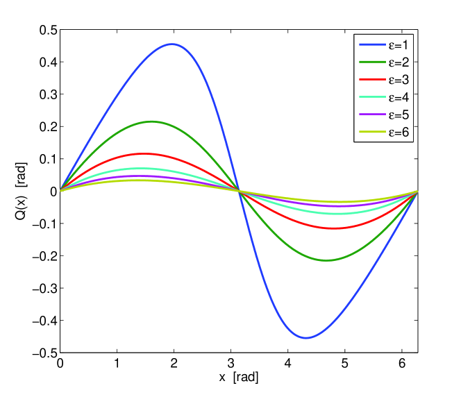
Figure 1: The shape of $\tanh$ type advance-delay phase response functions in equation (23).

From Theorem 4, we know in addition to the strength of the global and local cues, the phase response function of the global cue also determines the synchronization rate: the larger $\frac{Q_{g}(x)}{x}$ is, the faster the synchronization rate. In the following, we will show that the synchronization rate can be increased by designing $\varepsilon$, a parameter in the phase response function.

Theorem 5

For the pulse-coupled oscillator network in (8) and the phase response function of the global cue in the form of (23), if all $\xi_{i}$ are within $(-\pi,\pi)$, the synchronization rate increases with a decrease in $\varepsilon$, no matter whether the maximal/minimal $\xi_{i}$ is within or outside $(-\frac{\pi}{2},\frac{\pi}{2})$.

Proof:

According to Theorem 4, the synchronization rate increases with an increase in $\frac{Q_{g}(x)}{x}$. So we only need to prove that $\frac{Q_{g}(x)}{x}$ increases with a decrease in $\varepsilon$ for $x\in(-\pi,\,\pi)$.

Using the $\tanh$ type phase response function, we have

$$\frac{Q_{g}(x)}{x}=\frac{\tanh(x/\varepsilon)}{x\tanh(\pi/\varepsilon)}-\frac{1}{\pi},\quad x\in(-\pi,\,\pi)$$ (24)

Since $\frac{Q_{g}(x)}{x}$ in (24) is a smooth function of $\varepsilon$, we can calculate its derivative with respect to $\varepsilon$:

$$\frac{d(\frac{Q_{g}(x)}{x})}{d\varepsilon}=\frac{\pi\operatorname{sech}^{2}(\frac{\pi}{\varepsilon})\tanh(\frac{x}{\varepsilon})-x\operatorname{sech}^{2}(\frac{x}{\varepsilon})\tanh(\frac{\pi}{\varepsilon})}{x\varepsilon^{2}\tanh^{2}(\frac{\pi}{\varepsilon})}$$ (25)

To prove that $\frac{Q_{g}(x)}{x}$ increases with a decrease in $\varepsilon$, we need to prove that $\frac{d(\frac{Q_{g}(x)}{x})}{d\varepsilon}$ is negative. Since $\varepsilon^{2}\tanh^{2}(\frac{\pi}{\varepsilon})$ is positive, we only need to prove that (26) is negative for $-\pi<x<\pi$:

$$\frac{1}{x}\left(\pi\operatorname{sech}^{2}(\frac{\pi}{\varepsilon})\tanh(\frac{x}{\varepsilon})-x\operatorname{sech}^{2}(\frac{x}{\varepsilon})\tanh(\frac{\pi}{\varepsilon})\right)$$ (26)

Using properties of hyperbolic functions, we can rewrite (26) as follows:

$$\frac{4}{\left(e^{\frac{\pi}{\varepsilon}}+e^{\frac{-\pi}{\varepsilon}}\right)^{2}\left(e^{\frac{x}{\varepsilon}}+e^{\frac{-x}{\varepsilon}}\right)^{2}}$$ (27)

$$\times\ \frac{\pi\left(e^{\frac{2x}{\varepsilon}}-e^{\frac{-2x}{\varepsilon}}\right)-x\left(e^{\frac{2\pi}{\varepsilon}}-e^{\frac{-2\pi}{\varepsilon}}\right)}{x}$$

hence the problem is reduced to proving the negativity of $f(x,\varepsilon)$ in (28) for $-\pi<x<\pi$.

$$f(x,\varepsilon)\triangleq\frac{\pi\left(e^{\frac{2x}{\varepsilon}}-e^{\frac{-2x}{\varepsilon}}\right)-x\left(e^{\frac{2\pi}{\varepsilon}}-e^{\frac{-2\pi}{\varepsilon}}\right)}{x}$$ (28)

Using a Taylor expansion, equation (28) can be further rewritten as

$$f(x,\varepsilon) =\frac{1}{x}\left[2\pi\left(\frac{2x}{\varepsilon}+\frac{(\frac{2x}{\varepsilon})^{3}}{3!}+\frac{(\frac{2x}{\varepsilon})^{5}}{5!}+\ldots\right)\right.$$ (29)

$$\left.\qquad\quad-2x\left(\frac{2\pi}{\varepsilon}+\frac{(\frac{2\pi}{\varepsilon})^{3}}{3!}+\frac{(\frac{2\pi}{\varepsilon})^{5}}{5!}+\ldots\right)\right]$$

$$=\frac{2}{x}\left(\frac{\pi(\frac{2x}{\varepsilon})^{3}-x(\frac{2\pi}{\varepsilon})^{3}}{3!}+\frac{\pi(\frac{2x}{\varepsilon})^{5}-x(\frac{2\pi}{\varepsilon})^{5}}{5!}+\ldots\right)$$

which is negative for all $x$ in $-\pi<x<\pi$.

So $\frac{(\frac{Q_{g}(x)}{dx})}{d\varepsilon}$ is negative, thus $\frac{Q_{g}(x)}{x}$ increases with a decrease in $\varepsilon$, which completes the proof. ∎

VI QualNet Experiments

We use a high-fidelity network evaluation tool (QualNet) to illustrate the proposed strategy. QualNet is a commercial network platform that has been widely used to predict the performance of MANETs, satellite networks and sensor networks, among others [24].

In the implementation, we constructed a wireless network composed of 19 nodes (including 1 global cue). Each node has a counter as clock and stores the phase response function (as shown in Fig. 1) in a lookup table. Upon receiving a pulse, a node shifts its phase by an amount determined by its current time and the phase response function in the lookup table. The structure of the network is illustrated in Fig. 2, where node number 0 is the global cue. A broadcasting-based MAC layer protocol is adopted to establish the pulse based communication between different nodes, which is represented by the circles in Fig. 2. Although a broadcasting scheme is used, the communication in the network is not all-to-all due to limited transmission range. The interaction topology is also illustrated in Fig. 2, which can be verified to be a connected graph.

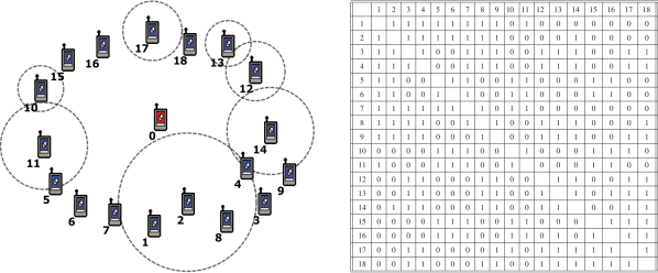
Figure 2: Schematic of the network (left) and interaction matrix (right) used in the QualNet implementation. In the interaction matrix, ‘1’ denotes interaction between two nodes, and ‘0’ denotes no interaction.

We first considered the case where $\xi_{i}\in(-\frac{\pi}{2},\frac{\pi}{2})$. From Theorem 1, all nodes can synchronize to the global cue if at least one $g_{i}$ is non-zero. To confirm the prediction, we only connected oscillator $1$ to the global cue with $g_{1}=0.01$. We set the natural frequency to $2\pi$, the strength of local coupling to $l=0.01$, and implemented the PCO network under different phase response functions in (23), i.e., different pairs of $\varepsilon_{g}$ ($\varepsilon$ in $Q_{g}$) and $\varepsilon_{l}$ ($\varepsilon$ in $Q_{l}$). The network was synchronized, confirming Theorem 1. To illustrate our phase-response-function based design strategy, we recorded the average time to synchronization from 100 runs for each pair of $\varepsilon_{g}$ and $\varepsilon_{l}$. In each run, we set the initial value of the global cue as $0$ and chose the initial values of local nodes randomly from a uniform distribution on $(-\frac{\pi}{2},\,\frac{\pi}{2})$. The times to synchronization are given by the first element of each 2-tuple in Table I. We can see that the synchronization rate increases with a decrease in $\varepsilon_{g}$, which confirms the theoretical results in Sec. V. The total energy consumption in the synchronization process is also recorded and averaged over the 100 runs. The results are given by the second element of each 2-tuple in Table I. With a decrease in $\varepsilon_{g}$, the energy consumption indeed decreases, which confirms the effectiveness of our design methodology in Sec. V.

TABLE I: Time to synchronization [s]($1$st element of each 2-tuple) and energy consumption [$10^{-3}$J]($2$nd element of each 2-tuple) under different phase response functions ($\xi_{i}\in(-\frac{\pi}{2},\,\frac{\pi}{2})$, $l=g_{1}=0.01$, $g_{2}=g_{3}=\ldots=g_{N}=0$)

$\varepsilon_{g}$ $\backslash$ $\varepsilon_{l}$	$0.05$	$0.1$	$0.2$	$0.4$	$0.8$	$1.6$
$0.4$	(37.23, 729.39)	(36.76, 719.99)	(36.55, 715.79)	(36.23, 709.05)	(35.83, 701.39)	(43.37, 852.19)
$0.8$	(37.88, 742.39)	(37.40, 732.79)	(37.88, 742.39)	(36.73, 719.39)	(36.44, 713.59)	(44.04, 865.59)
$1.6$	(38.17, 748.19)	(37.90, 742.79)	(38.38, 752.39)	(37.62, 737.19)	(36.83, 721.43)	(45.76, 899.99)

Using the same setup, we also implemented the network when the maximal/minimal $\xi_{i}$ is outside $(-\frac{\pi}{2},\,\frac{\pi}{2})$. We ran the implementation for 100 times and each time chose the initial values of $\xi_{i}$ randomly from a uniform distribution on $(-\pi,\,\pi)$. $28$ of the 100 runs were unsynchronized, confirming Theorem 2 that all oscillators have to be connected to the global cue to guarantee synchronization. So we made $g_{1}=g_{2}=\ldots=g_{N}=0.01$ and re-ran the implementation under different phase response functions. The results are given in Table II. With a decrease in $\varepsilon_{g}$, the energy consumption indeed decreases, confirming the effectiveness of our design methodology in Sec. V. Moreover, using the same coupling strength, we also implemented the network under Peskin’s phase response function used in [3], and obtained a (synchronization time, energy consumption) 2-tuple as $(25.24,\,489.59)$. Since it is larger than the smallest energy consumption in Table II, which is obtained under the same coupling strength, this confirms that by tuning the parameter $\varepsilon_{g}$ in phase response function, energy consumption can indeed be reduced.

TABLE II: Time to synchronization [s]($1$st element of each 2-tuple) and energy consumption [$10^{-3}$J]($2$nd element of each 2-tuple) under different phase response functions ($\xi_{i}\in(-\pi,\,\pi)$, $l=g_{1}=g_{2}=\ldots=g_{N}=0.01$)

$\varepsilon_{g}$ $\backslash$ $\varepsilon_{l}$	$0.05$	$0.1$	$0.2$	$0.4$	$0.8$	$1.6$
$0.4$	(22.93, 443.39)	(23.17, 448.19)	(23.14, 447.59)	(22.58, 436.39)	(21.53, 415.39)	(22.44, 433.59)
$0.8$	(24.95, 483.79)	(25.21, 488.99)	(25.36, 491.99)	(24.23, 469.39)	(23.63, 457.39)	(24.34, 471.59)
$1.6$	(30.14, 587.59)	(31.92, 623.19)	(31.75, 619.79)	(30.35, 519.79)	(28.15, 547.79)	(29.09, 566.59)

Setting $g_{1}=g_{2}=\ldots=g_{N}=g$, $\varepsilon_{g}=0.4$, and $\varepsilon_{l}=0.05$, we also implemented the network under different strengths of global and local cues, i.e., different pairs of $g$ and $l$. For each pair of $g$ and $l$, we ran the implementation for 100 times, and each time we chose the initial values of $\xi_{i}$ randomly from a uniform distribution on $(-\pi,\,\pi)$. The average time to synchronization is given by the first element of each 2-tuple in Table III. From Table III, we can see that a larger $g$ indeed leads to a faster synchronization rate (a smaller synchronization time), whereas a larger $l$ does not necessarily bring a faster synchronization rate. A larger $l$ may even desynchronize the network when $g$ is small (as illustrated by the last two elements of the first row). This confirms the analytical results in Remark 7, which state that the local cue may increase or decrease the synchronization rate. The same conclusion can be drawn for energy consumption, which is given by the second element of each 2-tuple in Table III.

TABLE III: Time to synchronization [s] ($1$st element of each 2-tuple) and energy consumption [$10^{-3}$J] ($2$nd element of each 2-tuple) under different strengths of global and local cues ($\xi_{i}\in(-\pi,\,\pi)$, $g_{1}=g_{2}=\ldots=g_{N}=g$)

$g$ $\backslash$ $l$	$0.01$	$0.02$	$0.03$	$0.04$	$0.05$	$0.06$
$0.01$	(22.93, 443.39)	(23.21, 448.99)	(26.37, 512.19)	(27.26, 529.99)	(no sync, $-$)	(no sync, $-$)
$0.02$	(17.49, 334.59)	(18.90, 362.79)	(22.03, 425.39)	(24.60, 476.79)	(24.38, 472.39)	(21.39, 412.59)
$0.03$	(14.18, 268.39)	(14.99, 284.59)	(18.03, 345.39)	(19.93, 383.39)	(20.35, 391.79)	(19.91, 382.99)

VII Conclusions

The synchronization rate of pulse-coupled oscillators is analyzed. It is proven that in addition to the strengths of global and local cues, the phase response function also determines the synchronization rate. This inspires us to increase the synchronization rate by choosing an appropriate phase response function when the phase response function is a design parameter. An application is the clock synchronization of wireless networks, to which pulse-coupled synchronization strategies have been successfully applied. By exploiting the freedom in the phase response function, we give a new design methodology for pulse-coupled synchronization of wireless networks. The new methodology can reduce energy consumption in clock synchronization. QualNet experiments are given to illustrate the analytical results.

References

- [1] R. Mirollo and S. Strogatz. Synchronization of pulse-coupled biological oscillators. SIAM J. Appl. Math., 50:1645–1662, 1990.
- [2] A. Abdrabou and W. Zhuang. A position-based QoS routing scheme for UWB mobile ad hoc networks. IEEE J. Sel. Areas Commun., 24:850–855, 2006.
- [3] Y. W. Hong and A. Scaglione. A scalable synchronization protocol for large scale sensor networks and its applications. IEEE J. Sel. Areas Commun., 23:1085–1099, 2005.
- [4] A. Tyrrell, G. Auer, and C. Bettstetter. Emergent slot synchronization in wireless networks. IEEE. Trans. Mob. Comput., 9:719–732, 2010.
- [5] G. Werner-Allen, G. Tewari, A. Patel, M. Welsh, and R. Nagpal. Firefly inspired sensor network synchronicity with realistic radio effects. In Proc. SenSys 05, pages 142 –153, USA, 2005.
- [6] R. Pagliari, Y. W. P. Hong, and A. Scaglione. Bio-inspired algorithms for decentralized round-robin and proportional fair scheduling. IEEE J. Sel. Areas Commun., 28:564 –575, 2010.
- [7] Y. Q. Wang, F. Núez, and F. J. Doyle III. Energy-efficient pulse-coupled synchronization strategy design for wireless sensor networks through reduced idle listening. IEEE Trans. Signal Process., Accepted.
- [8] Y. Q. Wang and F. J. Doyle III. On influences of global and local cues on the rate of synchronization of oscillator networks. Automatica, 47:1236–1242, 2011.
- [9] P. Delellis, M. di Bernardo, and M. Porfiri. Pinning control of complex networks via edge snapping. Chaos, 21:033119, 2011.
- [10] H. Kopetz and W. Ochsenreiter. Clock synchronization in distributed real-time systems. IEEE Trans. Comput., C-36:933–940, 1987.
- [11] E. Izhikevich. Dynamical systems in neuroscience: the geometry of excitability and bursting. MIT Press, London, 2007.
- [12] S. Barbarossa and G. Scutari. Bio-inspired sensor network design: Distributed decision through self-synchronization. IEEE Signal Process. Mag., 24:26 –35, 2007.
- [13] F. C. Hoppensteadt and E. M. Izhikevich. Weakly connected neural networks. Springer, New York, 1997.
- [14] T. S. Rappaport. Wireless communications: principles and practice. Prentice Hall, New York, 2002.
- [15] S. J. Park and R. Sivakumar. Load-sensitive transmission power control in wireless ad-hoc networks. In GLOBECOM, pages 42–46, Taibei, 2002.
- [16] C. V. Vreeswijk, L. F. Abbott, and G. B. Ermentrout. When inhibition not excitation synchronizes neural firing. J. Comput. Neurosci., 1:313–321, 1994.
- [17] H. K. Khalil. Nonlinear systems. Prentice Hall, New Jersey, 2002.
- [18] C. Godsil and G. Royle. Algebraic graph theory. Springer, New York, 2001.
- [19] R. Horn and C. Johnson. Matrix analysis. Cambridge University Press, London, 1985.
- [20] P. Monzón and F. Paganini. Global considerations on the Kuramoto model of sinusoudally coupled oscillators. In Proc. 44th IEEE Conf. Decision Control, pages 3923 –3928, Spain, 2005.
- [21] S. Chung and J. Slotine. On synchronization of coupled Hopf-Kuramoto oscillators with phase delays. In Proc. 49th IEEE Conf. Decision Control, pages 3181–3187, USA, 2010.
- [22] A. Tyrrell, G. Auer, and C. Bettstetter. Fireflies as role models for synchronization in ad hoc networks. In Proc. Int. Conf. Bio Inspired Models of Network, Information and Computing Systems (BIONETICS), pages 1–7, Italy, 2006.
- [23] B. Ermentrout. Type I membrances, phase resetting curves, and synchrony. Neural Comput., 8:979–1001, 1996.
- [24] QualNet 4.5 User’s Guide. Scalable networks inc. http://www.scalable-networks.com, 2008.