Electron-ion and ion-ion potentials for modeling warm-dense-matter: applications to laser-heated or shock-compressed Al and Si.

Abstract

The pair-interactions $U_{ij}(r)$ determine the thermodynamics and linear transport properties of matter via the pair-distribution functions (PDFs), i.e., $g_{ij}(r)$. Great simplicity is achieved if $U_{ij}(r)$ could be directly used to predict material properties via classical simulations, avoiding many-body wavefunctions. Warm dense matter (WDM) is encountered in quasi-equilibria where the electron temperature $T_{e}$ differs from the ion temperature $T_{i}$, as in laser-heated or in shock-compressed matter. The electron PDFs $g_{ee}(r)$ as perturbed by the ions are used to evaluate fully non-local exchange-correlation corrections to the free energy, using Hydrogen as an example. Electron-ion potentials for ions with a bound core are discussed with Al and Si as examples, for WDM with $T_{e}\neq T_{i}$, and valid for times shorter than the electron-ion relaxation time. In some cases the potentials develop attractive regions, and then become repulsive and ‘Yukawa-like’ for higher $T_{e}$. These results clarify the origin of initial phonon-hardening and rapid release. Pair-potentials for shock-heated WDM show that phonon hardening would not occur in most such systems. Defining meaningful quasi-equilibrium static transport coefficients consistent with the dynamic values is addressed. There seems to be no meaningful ‘static conductivity’ obtainable by extrapolating experimental or theoretical $\sigma(\omega,T_{i},T_{e})$ to $\omega\to 0$, unless $T_{i}\to T_{e}$ as well. Illustrative calculations of quasi-static resistivities $R(T_{i},T_{e})$ of laser-heated as well as shock-heated Aluminum and Silicon are presented using our pseudopotentials, pair-potentials and classical integral equations. The quasi-static resistivities display clear differences in their temperature evolutions, but are not the strict $\omega\to 0$ limits of the dynamic values.

I Introduction

Novel techniques of high-energy deposition on matter using high-energy short-pulse lasers as well as shock waves enable one to produce matter in a variety of novel states. They demand theoretical techniques adapted to many physical regimes. Such warm-correlated matter (WCM), and warm dense mater (WDM), include hot-nucleating nanocrystals we well as hot-dense radiative (HDR) plasmas cimarron . They have applications ranging from laser micro-machining, laser ablation Lorazo-Lewis03 , Coulomb explosions Lewis , inertial-confinement fusion (ICF), astrophysics Militzer12 and aero-space re-entry applications SGA89 . The material may be electrons and ions in a complex mixture of ionization states of low-$Z$ and high-$Z$ ions, e.g., H to U. The temperatures could be very high and yet high compressions could make the electrons degenerate or partially degenerate. Predictions of the thermodynamics, transport, radiative, and thermonuclear processes cimarron pose major challenges. Furthermore, ion temperatures $T_{i}$ may differ from the electron temperature $T_{e}$, and the quasi-equilibrium properties, relaxation and transport have to be updated within the time-scales and energy-scales of such two-temperature equilibria Ng2011 .

Modern electronic-structure methods provide in situ density-functional potentials incorporated into molecular dynamics (MD) simulations Car-Par85 . The all-electron, all-ion quantum calculations for simple systems provide ‘bench-marks’, usually at low temperatures and normal densities. Such methods become untenable at higher-$T$ where large numbers of partially occupied eigenstates have to be included. HDR plasmas, relevant to ICF provide a perspective of the problem. The complexity of WDM, compressions and temperatures involved call for simplifications without sacrificing accuracy. Thus molecular dynamics (MD), i.e., classical simulations, using various effective potentials have been a focus of some recent studies JonesMur07 ; YeZhaoZhen10 . Such methods were used in earlier work Ross80 , often with phenomenological or ‘chemical’ models for pair-interactions, and in recent studies as well HouY09 . Other authors have studied statistical potentials inclusive of quantum diffraction effects DuftyDutta arising from integrating out the electrons. A re-examination of potentials useful in the non-equilibrium context is needed.

We study two types of non-equilibrium (two-temperature) systems, viz., (i) generated by short-pulse lasers (the ion subsystem remains virtually unchanged while $T_{e}$ increases during the pulse period) and (ii) mechanical shocks. Here the electrons remain at $T_{e}$ while $T_{i}$ and the compressions change. Our approach has been to construct the charge distribution $n(r)$ around a nucleus immersed in the medium via the neutral-pseudoatom (NPA) density-functional theory (DFT) models, e.g., Ref. eos95 . The $n(r)$ is used to construct a local weak pseudopotential dependent on the density and temperature of the ambient environment. The pseudopotentials $U_{ei}(r)$ provide pair-potentials $U_{ij}$ and pair-distribution functions (PDFs) $g_{ij}(r)$. These provide the thermodynamics and transport properties of the system in a self-consistent manner. The dependence of the $U_{ei}$ on the system parameters arises because the effective core-charge $\bar{Z}$, the ionic-core radii $r_{c}$, etc., of the ion-configuration depend on the medium. A type of transferable pseudopotentials is available with popular simulation software. However, they assume frozen-core radii $r_{c}$ and an ionization $\bar{Z}$ consistent with normal densities and $T=0$. They are not transferable to highly compressed WDM states, or low electron degeneracies, as is well known and noted even recently by Mazevet el al. Mazevet07 . A more detailed approach that does not require defining a ‘core’ would be to use all-electron regularized pseudo-potentials based on norm-conserving (NC) or projector-augmented-wave (PAW) approaches. Such methods would be strongly computer-intensive and not useful for most WDM problems. They could serve to provide a new set of benchmarks that are beyond Quantum-Monte Carlo calculations, rather than serve actual WDM calculations.

Using such NC, PAW or ‘standard’ pseudopotentials requires solving the many-center Schrödinger equation, as implemented in major codes codes . The numerical simplicity needed for studying complicated WCM systems with many ionization states and components in different temperature states is lost. Hence we focus on simple linear-response potentials as in, e.g., Ref. eos95 . The ion subsystem can be treated using MD or via integral equations like the hyper-netted-chain (HNC), or the modified-HNC (MHNC Rosen ) method to exploit spherical symmetry. This works even for quantum electrons at $T=0$ via a classical map prl1 . Hence the present study is an extension to non-equilibrium (two-temperature) systems generated by short-pulse lasers or mechanical shock. The physics expressed in terms of pair-potentials and PDFs can be directly generalized to deal with $T_{e}\neq T_{i}$, i.e., two-temperature quasi-equilibria, using $g_{su}(r,T_{s},T_{u})$, where $s,u$ are electron or ion subsystem labels. Such generalizations can be formally justified in terms of the Bogolubov-Zubarev type of non-equilibrium theory elr0 . Within the time scales $\tau_{ei}$ where subsystem Hamiltonians $H_{e}$ and $H_{i}$ remain invariant, we can also justify the use of DFT for each subsystem.

Since laser-pulsed heating or shock-compression experiments begin at some reference density near room temperature, the pseudopotentials can be checked against experimental liquid-metal properties. We use such liquid-metal-adapted pseudopotentials, with pair potentials constructed from finite-$T$ response functions incorporating finite-$T$ local fields consistent with the sum rules and finite-$T$ exchange-correlation effects prbexc . Equilibrium and quasi-equilibrium WDM Aluminum and Si are studied in detail. Experimentally useful quantities accessible via these calculations are (a) pair-distribution functions and structure factors (b) thermodynamics, e.g., Hugoniots, subsystem free energies, etc. (c) static and dynamic liner transport coefficients, (d) energy-relaxation rates (e) X-ray Thompson scattering and other dynamical results. In this paper we address various aspects of (a)-(d) and leave (e) for a future study.

We also ask if the electron-ion pseudopotentials $U_{ei}(r)$ or the pair-potentials $U_{ii}(r)$ could be approximated by a Yukawa form $W_{ss^{\prime}}$, and compare them with more detailed potentials.

Here we note that DFT or Car-Parinello methods cannot calculate the electron-electron PDFs $g_{ee^{\prime}}(r)$, where $e,e^{\prime}$ are electrons (with spin indices included as needed). However, these electron-electron PDFs may be calculated using a well-tested classical-map technique (CHNC) prl1 ; ijqc11 , inspired by finite-temperature DFT itself. This is used in sec. II to obtain the fully nonlocal exchange-correlation free energy of electrons interacting directly with ions, rather than jellium. In sec. II we use the electron-electron pair-distribution functions $g_{ee}(\lambda,r,T)$, where $\lambda$ is a coupling constant, to evaluate the difference between the exchange-correlation free energy of electrons in jellium and in hot hydrogen via a fully non-local evaluation using a coupling constant integration of $g_{ee}(r,T)$ in hydrogen.

Section III presents the details of the pseudopotential and PDF calculations for ions with a core specified by the charge $\bar{Z}(T_{i})$ and the radius $r_{c}$. Results for equilibrium and quasi-equilibrium Al and Si WDMs are given. The section IV on transport properties addresses the meaning of a ‘static’ conductivity as the frequency independent limit of the two-temperature dynamic conductivity $\sigma(\omega,T_{i},T_{e})$. It is argued that there may be no physical meaning in the ‘static conductivity’ obtained by extrapolating $\sigma(\omega,T_{i},T_{e})$ to $\omega\to 0$, unless $T_{i}\to T_{e}$ as well. Calculations are presented for a possible candidate to a ‘quasi-static’ resistivity of laser-heated and shock-heated Aluminum, showing how they differ from each other and from the $T$-dependent equilibrium resistivity. Such results can be used to test if the physical models presented here provide a reasonably accurate picture of laser-pulse heated or shock-heated materials in the WDM regime.

II Non-local exchange-correlation calculations.

An important application of finite-$T$ DFT is to evaluate the exchange-correlation contribution $f_{xc}(T)$ per electron to the Helmholtz free-energy $f$ of a given electron distribution $n(r)$ at the temperature $T$. This is usually done in the local-density approximation (LDA) using the $f_{xc}(T)$ per unit volume of the uniform electron gas (UGE) as the input functional. Some authors have even approximated this with the $T=0$ UGE parametrization, even though good approximations to $f_{xc}$ from evaluations of finite-$T$ bubble diagrams Perrot-Fxc ; Batonrouge , the Iyetomi-Ichimaru (IYI) parametrization Ichimaru as well as the $f_{xc}(T)$ from CHNC have been available for sometime prbexc . The IYI scheme and the CHNC $f_{xc}$ agree well in typical WDM regimes of density and $T$.

In this section we present a fully non-local calculation of $f_{xc}$ at finite $T$ for a system of electrons interacting with a subsystem of protons, using classical potentials and pair-distribution functions as the ingredients of our calculation. The protons are in thermal equilibrium with the electrons, and have kinetic energy. However, no Born-Oppenheimer approximation is invoked. The ions are a system of classical particles and no classical map is needed. The proton free energy has a correlation contribution $F^{(p)}_{c}$ which gets automatically evaluated through the HNC procedure. It is a highly non-local quantity that cannot be evaluated in the LDA even as a first approximation, but we do not dwell on it here. In fact, the total free-energy given by CHNC was used to calculate a Deuterium Hugoniot in  Hug-H but the nature of the purely electronic part $f_{xc}(r_{s},T)=F_{xc}/N$, where N is the total number of electrons, was not examined there in detail. Here we high-light that aspect and concentrate on the electronic part of the exchange-correlation free energy $F_{xc}$.

The Hamiltonian of the system and its free energy calculation are similar to that of the electron gas, except that the unresponsive ‘jellium’ background is replaced by the proton subsystem. Thus

$$H = H^{0}_{e}+H^{0}_{p}+H_{ep}+H_{ee}+H_{pp}$$ (1)

$$F = F^{mf}_{e}+F^{mf}_{p}+F_{ep}+F_{xc}+F^{(p)}_{c}$$ (2)

Here the superfix mf stands for ‘mean-field’, and all the terms have an obvious meaning. Since the electron and proton densities are identical, the electron Wigner-Seitz radius $r_{s}$ is also the proton $r_{s}$. The classical map is needed only for the electrons. We have used the HNC version of the classical map prl1 , i.e., CHNC, for this calculation. In CHNC the quantum electrons (even at $T$=0) are treated as a Coulomb gas at a finite temperature dependent on $r_{s}$ and $T$. The electrons interact via the diffraction-corrected Coulomb potential plus a Pauli exclusion potential. The latter accurately reproduces the exchange hole in the parallel-spin $g_{ee}(r)$ Lado . The density ($\sim$ 0.8 g/cc) in this illustrative calculation is chosen so that we have a fully ionized e-p gas at a high compression and $r_{s}=1.5$ au. The treatment of ions with bound states may follow the methods for Si and Al given below.

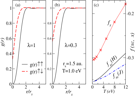
Figure 1: (Online color) (a)The parallel and anti-parallel electron pair-distribution functions $g_{ee}(r)$ at the full value of the Coulomb interaction, i.e., $\lambda$ = 1 in a system containing interacting protons and electrons at $r_{s}$ = 1.5 au. and $T$ = 1 eV. (b) The same PDFs evaluated at $\lambda$ =0.3, and for the same $r_{s},T$ as before. (c) The non-local exchange-correlation free energy $f_{xc}$ (solid line) in the hydrogen fluid, evaluated from the coupling-constant integration over the PDFs, compared with a similar calculation prbexc for jellium (dash-dot line) at $r_{s}$ = 1.5 and $T$ = eV. The exchange energy $f_{x}$ is evaluated from the PDFs at $\lambda=0$. Contributions to correlations from $g_{ep}(r)$ are not included here.

In the panels (a), (b) of fig 1, we display the electron pair-distribution functions $g_{ee}(\lambda,r,T)$ for values of the coupling constant $\lambda$ = 1, and 0.3. The Coulomb interaction $1/r$ is replaced by $\lambda/r$ with $\lambda$ varied from 0 to 1. The fully non-local exchange-correlation free energy per electron, $f_{xc}=F_{xc}/N$, is given by an integration of $h_{ij}(r)=g_{ij}(r)-1$ over $\lambda$.

$$f_{xc}=\frac{n}{2}\int_{0}^{1}\frac{d\lambda}{2\lambda}\int\frac{\lambda d{\vec{r}}}{r}[h_{11}(r,\lambda)+h_{12}(r,\lambda)].$$ (3)

It is noteworthy that the parallel-spin PDF, i.e., $g_{11}(r)$ is hardly affected by the value of the coupling constant. It is dominated entirely by the Pauli exclusion effect. Hence the correlations are mostly mediated by the anti-parallel $g(r)$ which changes drastically with $\lambda$. The success of the use of an ‘exact exchange’ in ‘optimized-effective potentials’ and related methods Krieger92 is related to this property of $g_{11}(r)$. Spurious ‘self-interaction’ errors are absent in CHNC implementations or any methods that directly use a $g(r)$. In panel (c) we present our values of $f_{xc}(H)$, i.e., the xc-free energy per electron in the presence of protons, and the corresponding quantity, labeled $f_{xc}(J)$ in the absence of protons, appropriate for the finite-$T$ jellium model. The exchange free energy $f_{x}$ is simply the exchange energy at $\lambda=0$, and is the same for the system with protons (Hydrogen) or without protons (i.e., jellium). Thus the correlation contribution is the many-body correction beyond the jellium $f_{x}$ at finite-$T$. The reference density matrix is diagonal in a set of plane-waves. The Hartree energy is zero. This definition of correlation energy is different to a treatment where the electron-proton fluid is treated as a system of hot atoms together with correlation corrections. There the correlation energy is usually defined with reference to a density matrix diagonal in an atomic Hartree-Fock basis. The corrections to the energy beyond the Hartree-Fock value are deemed the correlation energy. Such a basis already has electron-ion correlations in the wavefunctions which are not plane waves. They are not included in the $f_{xc}$ used here which is purely the electronic part. In effect, the correlation corrections in $g_{ei}(r)$ are differently partitioned in these different definitions, and hence care must be taken in making comparisons between atomic-like Hartree-Fock approaches to WDM sjostrom12 , and associated discussions of finite-$T$ correlation energies.

III The pseudopotentials.

Accurate pseudopotentials are available with standard computational packages codes , designed for condensed-matter applications where finite-$T$ effects, multiple ionizations, non-equilibrium effects etc., are uncommon. WCM applications require accurate but simpler potentials where classical simulations, linear response methods, etc., could be used instead of basis-set diagonalizations of a Hamiltonian. Here we consider (i) the simplest Yukawa type potentials, and (ii) more accurate pseudopotentials from DFT for a single nucleus immersed in a WDM medium. Thus a quantum calculation is necessary only for a single nucleus in a spherically symmetric environment modeled as a ‘neutral pseudo atom’ (NPA) eos95 . The ion density is at the ion temperature $T_{i}$. A DFT calculation at $T_{e}$ gives the electron density $n(r)$ around the nucleus, the effective ionic charge $\bar{Z}$, Kohn-Sham wavefunctions and phase-shifts.

III.0.1 The concept of $\bar{Z}$.

The core charge $\bar{Z}$, and the core radius $r_{c}$ are important parameters in the pseudopotentials discussed here. Some authors have expressed concern that $\bar{Z}$ is ‘not a well-defined physical quantity’, or that there is no quantum mechanical operator whose mean value is $\bar{Z}$. One may also note that there is no quantum mechanical operator whose mean value is the temperature $T$. Both $\bar{Z}$ and $T$ are Lagrange multipliers used to define relational properties. Pseudopotentials, and many other calculational quantities have the advantage of being definable with respect to a convenient reference $H_{0}$, but this does not mean any ‘arbitrariness’ in the theory. The $H_{0}$ selected in pseudopotential theory enables us to reduce a many-electron atomic problem to a few electron problem involving only $\bar{Z}$ electrons.

A properly constructed $\bar{Z}$ should satisfy (i) the neutrality condition $n_{e}=\bar{Z}n_{i}$, where $n_{i}$ is the ion density. That is, $\bar{Z}$ is the Lagrange multiplier whose value is chosen to ensures this neutrality condition. This is readily generalized to a mixture of ions with different charges $z_{j}$ (ii) the physical potential seen by a test charge in the plasma should tend to $\bar{Z}/r$ for large $r$, (iii) The $\bar{Z}$ should be consistent with the Friedel sum rule based on the phase-shifts from the ion with a charge $\bar{Z}$ and a core radius $r_{c}$. Finally, it has to be consistent with the set of bound states attached to the nucleus. These issues are discussed in Refs. hyd0 ,elr0 and provide a stringent set of constraints in choosing $\bar{Z}$. We have found that these constraints could generally be well satisfied within finite-$T$ DFT calculations that use a sufficiently large correlation sphere as the calculational volume. It has to be recognized that a material system, e.g., an Aluminum WDM, could be a mixture of many ionization states, e.g., $Al^{z_{j}+},z_{j}$ =$\cdots-1,0,1,2,3\cdots$ etc., where all ionization states are integers and correspond to different descriptions of the core, with different values of $r_{c}$. The concentrations of each species would be such as to minimize the total free energy if it is an equilibrium system elr0 .

III.0.2 Yukawa potentials.

The commonly used finite-$T$ Thomas-Fermi potentials, also called Yukawa potentials, are simple two-parameter forms. The core charge of the ions is $\bar{Z}$ and $r_{c}$ is set to zero (i.e., point ions). The field electrons are characterized by a screening wavevector $K_{Y}$.

$$W(r)_{ei} = -Z_{Y}/r$$ (4)

$$W(r)_{ii} = (Z^{2}_{Y}/r)\exp(-K_{Y}r)$$ (5)

We use atomic units with $|e|=\hbar=m_{e}=1$, and the temperatures are in energy units. If the electron temperature is $T_{e}$, the Thomas-Fermi electron-ion screening constant $K_{Y}$ is given by

$$K^{2}_{y} = \frac{4}{\pi T_{e}}\int_{0}^{\infty}k^{2}dkn(k)\{1-n(k)\}$$ (6)

$$n(k) = 1/\left[1+\exp\{(k^{2}/2-\mu)/T_{e}\}\right]$$ (7)

Here $\mu$ is the electron chemical potential at $T_{e}$ for the electron density $n_{e}$ consistent with the ionization $\bar{Z(T_{i},Te)}$. In the simplest theory $\bar{Z}$ is determined via finite-$T$ Thomas-Fermi theory. The structure factor consistent with this type of theory is:

$$S_{y}(k)=k^{2}/(k^{2}+K^{2}_{Y})$$ (8)

III.0.3 DFT-based linear-response pseudo-potentials.

The one-electron density is the essential functional that determines the equilibrium properties of a quantum system. Hence the electron density $n(r)$ around a nucleus of charge $Z$ placed in a uniform electron fluid at the bulk density $n_{e}$ and temperature $T_{e}$ is computed. The computational codes for such calculations have been available at least since Lieberman’s Inferno code Liberman , and extended recently as in Purgatorio Purgatorio . Most such codes use a single ion in a Wigner-Seitz cell of radius $r_{ws}=\{3/(4\pi\rho)\}^{1/3}$ as the computational volume when the ion density is $\rho$. In contrast, we use a large correlation sphere typical of the ion-correlations in the WDM. The single ion is surrounded by its self-consistent ion distribution $\rho(r)$ and the corresponding electron distribution $n(r)$, calculated self-consistently hyd0 . A correlation sphere of radius $R_{c}$ of 5 to 10 times $r_{ws}$ is used where $g_{ii}(R_{c})\to 1$. In most cases one may use the simplified form due to Perrot, where the ions are replaced by a uniform neutralizing background except for a cavity around the nucleus Pe-Be to mimic the ion-ion PDF. Further justification of this ‘neutral- pseudo-atom’ (NPA) model is given in ref. eos95

A weak local (i.e., $s$-wave) pseudopotential $U_{ei}(q)$, where $q$ is the wave vector is calculated from the free-electron density ‘pile-up’ $n_{f}(r)$ obtained via the finite-$T$ Kohn-Sham equation. This $n_{f}(q)$ is the density pile-up corrected in NPA eos95 for the cavity placed around the nucleus to simulate the ‘cavity’ of the $g_{ii}(r)$. Thus

$$\Delta U_{ei}(q)=n_{f}(q)/\chi_{ee}(r_{s},T_{e},q)$$ (9)

Here $\chi(r_{s},T_{e},q)$ is the electron linear-response function at the electron Wigner-Seitz radius $r_{s}$, and temperature $T_{e}$. A finite-$T$ local-field correction (LFC) $G_{q}$ is also needed to go beyond the simple random-phase approximation. That is,

$$\chi_{ee}(q) = \chi^{0}(q)/\{1-V_{q}(1-G_{q})\chi^{0}(q)\}$$ (10)

$$G_{q} = \{1-\gamma_{0}/\gamma\}(q/k_{TF})^{2}$$ (11)

$$V_{q} = 4\pi/q^{2},\;k_{TF}=(6\pi n/E_{F})^{1/2}$$ (12)

Here $\chi^{0}(q)$ is the non-interacting finite-$T$ Lindhard function. An electron effective mass $m^{*}$ (a ‘band mass’) is used in evaluating the Lindhard function. Thus, for Liquid Al near its melting point (m.pt., 0.081eV), $m^{*}=0.998$ gives good agreement of the calculated $S(k)$ with experiment Waseda . At higher temperatures $m^{*}=1$. The LFC $G_{q}(T_{e})$ is taken in the LDA (i.e., the $q\to 0$ form is used for all $q$), and evaluated from the ratio of the non-interacting and interacting finite-$T$ compressibilities $\gamma_{0}$ and $\gamma$ respectively. Alternatively, $G_{q}$ with full $q$-dispersion consistent with the $S(k)$ obtained from the PDF $g_{ee}(r)$ may be used, as discussed in Ref. prl1 . However, the formulation in terms of the $q\to 0$ given in Eq. 11 is quite accurate for the systems studied here.

Instead of numerical tables obtained from Eq. 9, a simple fit to the $U_{ei}(q)$ may be used. The fits used here are the Heine-Abarankov (HA) forms HA-ref , or a slight generalization by Dharma-wardana and Perrot elr0 . The two elements Al and Si chosen for this study only need a well-depth parameter $D$, and $r_{c}$ which is the core radius. The electron effective mass (i.e., band mass) $m^{*}$ enters into the response function.

$$U_{ei}(r) = -\bar{Z}D/r_{c},\;\;r\leq r_{c}$$ (13)

$$= -\bar{Z}/r,\;\;r>r_{c}$$ (14)

$$U_{ei}(q) =- \bar{Z}V_{q}M(q)$$ (15)

$$M(q) = D\sin(qr_{c})/qr_{c}+(1-D)\cos(qr_{c})$$ (16)

Furthermore, it is found from test calculations that the scaled quantities $D/(\bar{Z}/r_{ws})$, $r_{c}/r_{ws}$ could be treated as constants for changes in $r_{ws}$ if $\bar{Z}$ remains unchanged. This enables us to explore the behaviour of these WDMs for compressions deviating significantly from unity, without having to do full DFT-calculations in each case. The use of a suitable electron-effective mass $m^{*}$ bypasses the complications of ‘non-local’ pseudopotentials and provide excellent results with just $s$-wave potentials. Usually $m^{*}$ can be set to unity. It also may be used as a parameter fine tuned to get agreement with experimental $S(k)$ data, or in fitting a pseudopotential to $n_{f}(q)$ obtained from a DFT calculation, as in Eq. 9.

The NPA approach to simple local pseudopotentials is reliable if the resulting $U_{ei}(q)$ is such that

$$U_{ei}(q)/(-\bar{Z}V_{q})\leq 1.$$ (17)

III.1 Equilibrium pair potentials.

We present illustrative numerical results for Al and Si potentials with $T_{e}=T_{i}=T$. The screened pair-potential $U_{ii}(q)$ is calculated from the pseudopotential via:

$$U_{ii}(q)=\bar{Z}^{2}(T)V_{q}+|U_{ei}(q)|^{2}\chi_{ee}(q,r_{s},T)$$ (18)

Further improvement of these formulae to incorporate core-polarization effects etc., via DFT are discussed in the appendix of Ref. eos95 .

Potentials for calculations with C, Si, and Ge in the equilibrium WDM regime have been discussed by Dharma-wardana and Perrot in Ref. csige90 , and for Al for $T>5$ eV in Ref. elr0 . The normal-density liquid-metal Al pseudopotential used here is the potential discussed in Ref. Dharma-Aers83 . This $U_{ei}(q)$ generates the DFT $n(q)$ under linear response and recovers experimental $S(k)$ data quite well.

Pair potentials of other elements and at most compressions can be evaluated as in Ref. Pe-Be . Numerical results for $\beta U_{ii}(r)$, $\beta=1/T$ are displayed in Fig. 2. They are are particularly interesting in view of the subsidiary $2k_{F}$ peak in $S(k)$. Solid silicon has a rather open structure (diamond-like) which collapses under melting into a high-density metallic fluid. Car-Parinello simulations, many-atom Stillinger-Weber type potentials (requiring many empirical parameters) etc., need to be highly elaborate to capture the subsidiary structure associated with the electron mass $m^{*}$ and the 2$k_{F}$ scattering processes. In fact, attempts were made in some of these early MD studies to explain this ‘hump’ in the Si-$S(k)$ in terms of covalent bonds between Si atoms. In reality, molten Si is an excellent metal and the ‘hump’ is a metallic property associated with $m^{*}(k)$. In our view, two-center bonding effects do not arise unles electron densities fall to low values (e.g., 1/64 of the normal electron density for Al), and the temperatures become sufficiently low.

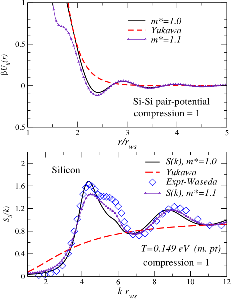
Figure 2: (Online color).(top) The Si-Si pair-potentials $\beta U_{ii}(r)$, $\beta=1/T$, at the melting point ($T_{i}=T_{e}=T=0.15$ eV) at unit compression ($r_{ws}$=3.07au), using an empty-core pseudopotential with core radius $r_{c}/r_{ws}$ =0.3084 are displayed for electron effective masses $m^{*}=1$, and 1.1. The Yukawa potential 5 is also displayed. (Bottom panel) The corresponding ion-ion structure factors $S_{ii}(k)$, as well as the experimental data of Waseda Waseda are shown. The additional structure near the Kohn anomaly ( 2$k_{F}$) beyond the main-peak is very sensitive to the local band mass $m^{*}$

WDM systems generated from laser pulsing or shock compression usually starts from a solid-density. Thus the pseudopotentials and pair-potentials should successfully recover the strongly-correlated low-temperature regime near the melting point (m.pt), as well as the higher-$T$ and $\kappa$ regimes. Our Al-Al pair potential at the m.pt is shown in the inset to Fig. 3, together with the DRT potential (based on a non-local pseudopotential) which is known to recover the properties of solid and liquid Al at low-temperatures DRT .

It is seen that the Yukawa potentials approximately reproduces the envelope of the pair-potentials, while failing to reproduce the Friedel oscillations and energy minima. Similarly, the Yukawa structure factor $S_{y}(k)$ does not have oscillatory features.

III.1.1 Pair-potentials for mixtures.

Many WDM systems involve mixtures of ions. Thus plastic converts to a compressed WDM containing mostly a mixture of H, C, O ions. Even an Aluminum plasma could contain several stages of ionization and they have to be treated as a mixture. The detailed treatment of such systems as mixtures of average atoms, their chemical species-dependent potentials, embedding energies etc., as well as pair-potentials were discussed in Ref. eos95 . The pair potential involving two types of ions carrying mean charges $\bar{Z}_{a},\bar{Z}_{b}$ could be written as

$$U_{a,b}(q)=V_{q}\bar{Z}_{a}\bar{Z}_{b}+|U_{ea}(q)U_{eb}(q)|\chi_{ee}(q)$$ (19)

Such cross-potentials would be inputs to the MHNC equations, or to MD simulations, for generating the corresponding PDFs.

III.2 Non-equilibrium pair-interactions.

In the following we examine two-temperature quasi-equilibrium systems rather than full non-equilibria. Such systems occur during times $t$ such that $\tau_{ee}<\tau_{ii}<t<\tau_{ei}$, after the energy is dumped in either the ion subsystem (mechanical shock) or in the electron subsystem (by a laser pulse).

III.2.1 Laser-pulse generated quasi-equilibria.

When a metal foil at the bath-temperature $T_{b}$ is subject to a short-pulse laser, the electron temperature rises rapidly to some $T_{e}$ within femto-second times scales $\tau_{ee}$, by equilibration via electron-electron interactions. The transfer of energy to the ion subsystem, arising from electron-ion interactions is slow, and hence the ion temperature $T_{i}$ remains essentially locked to $T_{b}$, while the electrons reach $T_{e}$. Hence, processes occurring within the electron-ion temperature relaxation timescale $\tau_{ei}>t>\tau_{ii}$ may be probed to provide information about quasi-equilibrium systems. The probes are optical pulses sampling a volume related to a space-time average over the pulse time and the optical depth of the material. Hence the ‘experimental results’ reported should be regarded as already implicitly containing some sort of interpretational model.

A proper description of such systems needs pair-potentials $U_{ii}(r,T_{e},T_{i})$ where $T_{e}\neq T_{i}$. The procedure described for the equilibrium system can be simply generalized for quasi-equilibria. In laser-heated systems, the pseudopotential is that of the initial state $T=T_{i}=T_{e}$, and this remains unchanged under changes of $T_{e}$ as long as $\bar{Z}$ remains unchanged. Unlike in the equilibrium case, the bare ion-ion pair potential in a laser-heated metal is screened by the (hot) electrons at $T_{e}$. Hence,

$$U_{ii}(q,T_{i},T_{e})=\{\bar{Z}(T_{i})\}^{2}V_{q}+|U_{ei}(q,T_{i})|^{2}\chi_{ee}(q,r_{s},T_{e})$$ (20)

The ion-ion structure factors $S(k)$ is that of the initial state at $T=T_{i}=T_{e}$ for time scales shorter than $\tau_{ei}$.

The main part of Fig. 3 shows the evolution of the potentials under laser-pulsed heating where $T_{e}$ increases while the ion subsystem remains intact for time scales shorter than $\tau_{ei}$. The first minimum near $r/r_{ws}\sim 1.85$ (marked A) weakens at first, and then deepens for $T_{e}>\sim 0.08$ eV (with $T_{i}$ fixed at 0.03 eV). This is clearly evident for the case $T_{e}=0.5$ eV in the figure. This may be considered a microscopic signature of ‘phonon hardening’ observed in some experiments Ernstorfer09 .

The highest phonon frequency $\omega_{ph}$ supported by the Al-lattice at 90K is $\sim 6\times 10^{13}$ s^-1, while this decreases rapidly at higher temperatures, and becomes purely imaginary if the lattice melts. The concept of a ‘phonon’ may not become meaningful if $1/\omega_{ph}$ begins to exceed $\tau_{ei}$. In fact, the two-temperature pair-potential itself requires updating at each time step.

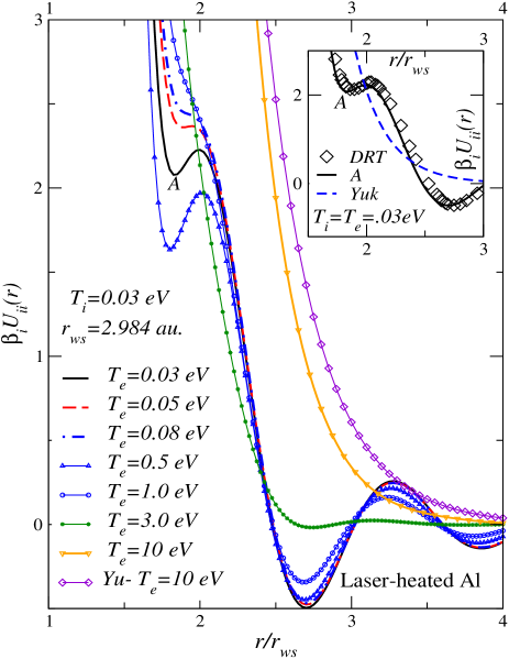
Figure 3: (Online color). (Inset) The Al-Al pair-potential, $\beta_{i}U_{ii}(r)$, $\beta_{i}=1/T_{i}$, at room temperature ($T_{e}=T_{i}=T$ = 0.03 eV) and normal density, labeled A is derived from a two-parameter local pseudopotential and a band mass $m*=1.02$. It is compared with a well established non-local potential  DRT that accurately reproduces structural and phonon data of Aluminum. The Yukawa potential, Eq.  5, at $T=0.03$ eV is also displayed. The main panel displays the evolution of the potential while $T_{i}$ is held fixed at 0.03 eV, and $T_{e}$ is increased. The potential becomes repulsive from $T_{e}=$0.03 eV to 0.08 eV. For $T_{e}>0.08$ eV it deepens and becomes attractive, e.g., at $T_{e}=0.5$ eV, before it finally becomes repulsive. The Yukawa potential at $T_{e}=10$ eV is also shown

When the electron temperature rises above $\sim 1$ eV, the potentials (see Fig. 3) become repulsive and the resulting compression in the electron subsystem increases rapidly, leading to a ‘Coulomb explosion’. We have assumed that $T_{e}$ is not sufficiently high to open up an ionization channel that would add to the energy relaxation between cold ions and hot electrons. Such processes may be addressed as in Ref. mmll .

III.2.2 Shock generated quasi-equilibria

The time evolutions of $T$ and $\kappa$ in shock-compressed systems are quite different to those of laser-heated samples. The Hugoniot is the locus of states that can be reached by a single shock wave, providing a relation connecting the volume, internal energy and the compression. Well-developed mathematical and numerical techniques exist for shock studies, if the equation of state (EOS) is available Swift07 . The Hugoniot prevails only after many time steps greater than $\tau_{ei}$. We are interested in shorter quasi-equilibrium time scales. Experimentally, the temperature evolution of the ion subsystem is very difficult to measure, and the temperature deduced from the thermal emissivity of the shocked state is for the state following hydrodynamic interactions between the sample and the observation window.

Thus material properties of the shocked state is determined from optical measurements combined with velocities of shock fronts and particles. The ‘sample region’ (seen by the optical probe) is the layer of material within approximately one optical depth behind the shock front (assuming that we are observing a shock wave in-flight inside the sample with no release wave). For a typical optical depth of $\sim$ 5 nm, and shock speeds of $\sim 10^{4}$ m/s, the transit time $\tau_{sh}$ of the shock front through this layer is $\sim$ 0.5 ps AndrewNg12 . Since $\tau_{ee}<<\tau_{sh}$, there is a meaningful $T_{e}$ in the sample region. In any case no energy has been dumped into the electron subsystem for $t<<\tau_{ei}$. Since the phonon frequency of typical solids is of the order of several THz (i.e., $\tau_{ii}<\tau_{sh}$), one may assume that the ion subsystem can be characterized by a temperature $T_{i}$. This would lead to a single two-$T$ quasi-equilibrium in the sample volume, or possibly a gradient of such quasi-equilibria in $T_{e}$ and $T_{i}$ along the path behind the shock front. In either case, we need two-temperature pair-potentials along a non-equilibrium ‘Hugoniot’.

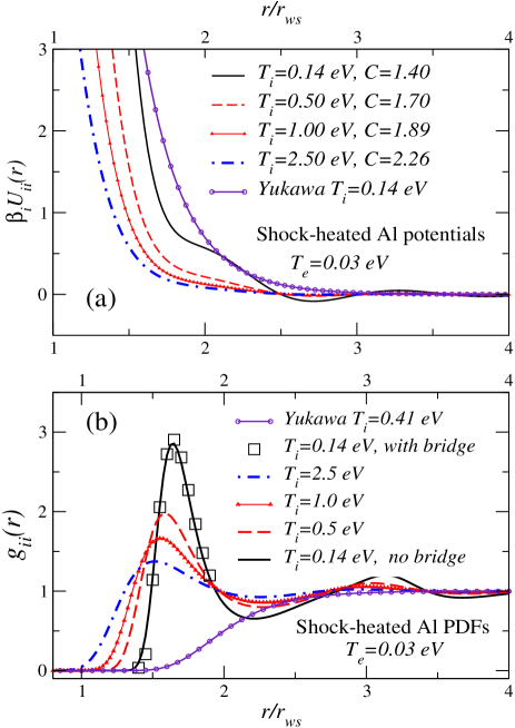
Figure 4: (a)The pair-potentials $\beta_{i}U_{ii}(r),\beta_{i}=1/T_{i}$ for a shock-heated Aluminum WDM with an initial temperature of $T_{e}=0.03$ eV, with the ion-subsystem temperature increasing to 2.5 eV. (b) The corresponding ion-ion PDFs $g_{ii}(r)$ where $T_{e}$ remains fixed at 0.03 eV, while $T_{i}$ increases to 2.5 eV as displayed. Calculations with bridge (MHNC) and without bridge corrections (HNC) are given for $T_{i}=0.14$ eV, showing that bridge corrections are negligible. The other PDFs are HNC solutions. The Yukawa PDF is the Boltzmann form.

We model this system as follows. Here the usual EOS is a good approximation to the quasi-EOS mainly because the energy in the electron system is small compared to that of the ions. Electrons remain more or less degenerate even at $T_{i}$=10 eV, when the compression reaches $\sim 3$. If $\kappa$ remains within a region where $\bar{Z}$ is unchanged, the bound electrons remain intact. However, in general the value of $\bar{Z}$ appropriate to the compression must be used and energy-relaxation by ionization need to be considered mmll . The compressions are calculated from Al and Si Hugoniots where we may neglect the small differences in the contribution to the internal energy from the electron subsystem at equilibrium or at quasi-equilibrium. The Al Hugoniot is based on our neutral-pseudoatom calculations eosbenage . The Si Hugoniot Stern is the L140 data based on the Quotidian-EOS model L140 .

The onset of compression makes the potential take a Yukawa form except at very low-energy deposition. This pair-potential does not support phonons or ‘phonon hardening’ at the accessible short-times scales, or at longer time scales. In this problem the ion-electron time scales $\tau_{ei}$ are lengthened due to the formation of ion-acoustic coupled modes involving both electrons and ions (hence the life times of the two-$T$ quasi-equilibria become longer).

Table 1: The temperature $T_{i}$ (eV) and compression $\kappa$, for shock-compressed aluminum and Si, for an initial normal density and temperatures $T_{e}$ = $T_{i}$ = 0.03 eV. The ionization $\bar{Z}$ remains essentially at 3 for Al, and 4 for Si. The electron temperature $T_{e}$ remains at the initial temperature for time scales less than $\sim\tau_{ei}$.

$T_{i}(eV)$	0.14	0.25	0.50	1.00	2.50	5.00
$\kappa$-Al	1.4	1.57	1.70	1.89	2.26	2.59
$\kappa$-Si	1.57	1.70	1.87	2.14	2.65	3.07

Figure 4 shows the pair-potentials (upper panel) and the corresponding two-temperature pair-distribution functions obtained by this procedure for Al. No bridge corrections have been included in the $g(r)$ shown in Fig. 4 except for $T_{i}=0.14$ eV, $T_{e}$ = 0.03 eV, where it is shown that their effect is negligible. The Yukawa PDF is taken as the Boltzmann form $\exp\{-W_{Y}(r)/T_{i}\}$.

One may wonder whether potentials beyond binary-interactions would be necessary in a classical representation of a many-particle system. Attempts to simulate classical fluids with model potentials (e.g., Lennard-Jones) show that binary interactions are often inadequate. However, since the potentials were made out of Coulomb interactions in a systematic manner using DFT densities, we believe that such effects are not significant, and probably get included in the problem of modeling the bridge functions. However, this needs further study, as it could be important in low-density, low temperature systems, and near the critical point DW-Aers-Kr ; Rosen-Kahl97 .

IV two-temperature transport coefficients.

The transport coefficients that are of common interest are associated with weak applied gradients in the electric potential, temperature etc., so that linear transport coefficients like the electrical conductivity $\sigma_{e}$ and heat conductivity $\sigma_{h}$ could be defined. However, if the non-equilibrium system is such that the subsystem Hamiltonians $H_{e}$, $H_{i}$ are invariant only for time scales $\tau_{ee}$, $\tau_{ii}$, then the $\omega\to 0$ limit of the transport coefficients, i.e., their static values are not defined in any strict sense. Thus extrapolations of experimental data to the $\omega\to 0$ have to be carefully examined to understand their physical content. We refer to any processes with a time scale $\tau$ such that $\tau_{ii}<\tau<\tau_{ei}$ as quasi-static.

Thus these experiments need to be planned, keeping in mind the available lifetimes for experimentation. Evaluating energy-relaxation lifetimes $\tau_{ei}$ from the e-i pseudopotentials and dynamic response functions is itself an extremely demanding task elr0 ; mmll but needed in WDM studies. We note that if the Al-pseudopotential discussed here is used at unit compression, $T_{i}$ = 0.1 eV, $T_{e}=$ 1.0 eV, then $\tau_{ei}$ is $\sim 6.02\times 10^{6}$ electron-plasma oscillations long, while at $T_{i}$ = 0.1, $T_{e}$ = 5 eV this reduces to $\sim 0.72$ of the value at $T_{e}=1$ eV. These numbers are based on our formula for the energy-relaxation rate evaluated via the f-sum rule mmll , without including coupled-mode effects.

Here we examine the theory of the dynamic two-temperature conductivity as a typical example. The objective is to extract a frequency-independent (i.e., quasi-static) component, and present numerical calculations for the quasi-static part of the resistivity using the pseudopotentials and PDFs developed in the previous sections. This analysis puts a different perspective on the physical content of the two-temperature Ziman formulae that have been used in the past for these systems. The extent of its physical validity has to be established by experiment.

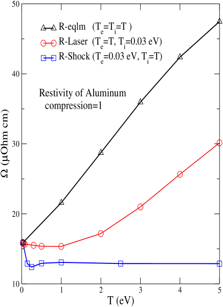
Figure 5: (Color online). Triangles: the equilibrium static resistivity of Aluminum at normal compression when $T=T_{e}=T_{i}$ increases from the melting point. Circles: the evolution of the quasi-static component of the dynamic resistivity (Eq. 25) of WDM-Aluminum at the melting density, with the ion-temperature $T_{i}$ held at 0.03 eV while the electron temperature $T_{e}$ is increased, as in laser-heated WDMs. Squares: the corresponding quasi-static resistivity for a shock-heated Al-WDM where $T_{e}$ remains fixed at 0.03 eV, while $T_{i}$ increases to 5 eV with compression, where $\kappa$ increases from 1.0 to $\sim 2.6$ .

The response time of the system to the probe has to be smaller than the system relaxation time $\tau_{ei}$, and long enough for the particle distributions to become stationary under the probe field. If a quasi-static electric field $\vec{E}$ is applied to an electron distribution $n(k)$, where $k$ is a wave vector, then it is the displaced stationary distribution $n(k,E)=n(k)+\delta(k,\vec{E})$ that determines the electrical conductivity of the system. The probe speed has to be consistent with the formation of a steady-state displaced-electron-distribution $n(k,\vec{E})$ in the electron system. The probe frequency cannot be slower than $1/\tau_{ei}$. Hence quantities obtained by extrapolating $\omega\to 0$ may not have a physical meaning.

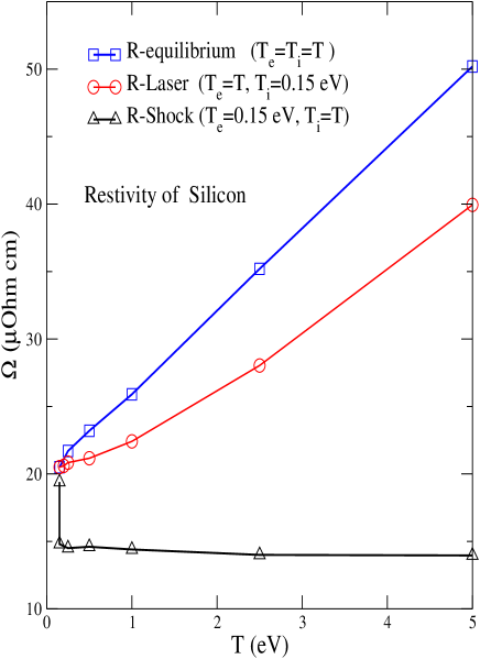
Figure 6: (Color online). Triangles: the equilibrium static resistivity of Si at normal compression when $T=T_{e}=T_{i}$ increases from near the melting point. Circles: the evolution of the quasi-static component of the dynamic resistivity (Eq. 25) of WDM-Si at the melting density, with the ion-temperature $T_{i}$ held at 0.15 eV while the electron temperature $T_{e}$ is increased, as in laser-heated WDMs. Squares: the corresponding quasi-static resistivity for a shock-heated Si-WDM where $T_{e}$ remains fixed at 0.15eV, while $T_{i}$ increases to 5 eV with compression, where $\kappa$ increases from 1.0 to $\sim 3$.

The measured conductivity can be associated with a scattering time $\tau(\omega)$ by writing

$$\sigma(\omega)=\frac{ne^{2}\tau(\omega)}{m_{e}\{1-i\omega\tau(\omega)\}}.$$ (21)

Here we have restored the electron charge and mass although we use atomic units. The conductivity $\sigma(\omega)$ can be expressed in terms of the Fourier component at the frequency $\omega$ of the current-current correlation function $<<J(t),J(t^{\prime})>>$. A standard evaluation, assuming that the effect of the total system is a superposition of the effect of individual scatterers can be carried out, as in the equilibrium case Mahantxt , but using the Keldysh contour for the non-equilibrium case. Here we keep in mind that the subsystem temperatures are $T_{e}$ and $T_{i}$, giving the result:

$$\frac{1}{\tau(\omega)} = -\frac{1}{(\omega^{e}_{p}m_{e})^{2}\omega}\int_{0}^{\infty}\frac{q^{2}dq}{(2\pi)^{3}}|U_{ei}(q,r_{s},T_{e})|^{2}q^{2}_{z}$$ (22)

$$\times\int_{0}^{\infty}\frac{d\nu}{2\pi}Im\{\chi_{ii}(q,\nu,r_{ws},T_{i})\}\Delta N(\nu,\omega)$$

$$\times Im\{1+V_{q}\chi_{ee}(q,\omega+\nu,r_{s},T_{e})\}$$

$$\Delta N(\nu,\omega) = [N((\nu+\omega)/T_{e})-N(\nu/T_{i})]$$ (23)

The last line contains Bose occupation factors $N\{(\nu+\omega)/T_{e}\}$ and $N(\nu/T_{i})$. Here $U_{ei}(q,r_{s},T_{e})$ is the pseudopotential presented in Eqs. 9-13. The frequency-dependent ion response function and the electron response function also appear. The latter was discussed in Eq. 10. The ion-response function can be constructed in a similar manner, or obtained from an MD simulation Jacucci .

This expression for the dynamic conductivity or $\tau(\omega)$ differs significantly from the Green-Kubo (GK) form used by a number of authors mazevet since both electron-electron and ion-ion many-body effects are treated dynamically in Eq. 22. In particular, in the currently available GK implementations, the Green-Kubo formula is averaged within an ensemble of static configurations generated by ion molecular dynamics; the electrons are quenched to a Born-Oppenheimer surface to evaluate one-electron Kohn-Sham eigenvalues which are used in the GK formula. The latter actually calls for eigenvalues of the Dyson equation. The ’quenching process’ destroys dynamical information; the ions and electrons ‘do not know’ each other’s temperatures.

We extract a meaningful ‘static’ component of the quasi-equilibrium dynamic resistivity as this has been the object of recent experiments, e.g., in Ref. NgAu . The physically meaningful lowest value $\omega_{L}$ of the probe frequency $\omega$ is $\sim 1/\tau_{ei}$. Hence, when $T_{e}$ is not strongly different from $T_{i}$ we may use $\omega=\omega_{L}$ in a Taylor expansion to write:

$$\Delta N(\nu,\omega)=N(\nu/T_{e})-N(\nu/T_{i})+\omega\frac{\partial N(\nu/T_{e})}{\partial\nu}+\cdots$$ (24)

The leading term in Eq. 24 is zero in the equilibrium case $T_{e}=T_{i}$. It is seen that the first-derivative term gives the Ziman resistivity in the equilibrium case, where an $\omega\to 0$ limit exists. When $T_{e}\neq T_{i}$, the first term in $\Delta N$ is non-zero and leads to a divergence unless $\omega$ remains finite. Thus the concept of a static conductivity is non-physical unless this ‘zeroth-order’ correction could be deemed negligible.

Replacing $\omega$ by its least allowed value $\omega_{L}\sim 1/\tau_{ei}$ in the above equation and in the pre-factor in Eq. 22, we obtain a frequency-independent first-order contribution. This can be further reduced to a two-temperature Ziman resistivity of the form:

$$R(T_{e},T_{i}) = \frac{\rho(T_{i})}{3\pi n(T_{e})}\int_{0}^{\infty}d\epsilon\frac{df(\epsilon)}{d\epsilon}\int_{0}^{2\surd{\epsilon}}S_{ii}(q,r_{ws},T_{i})$$ (25)

$$\times\left|\frac{U_{ei}(q,r_{s},T_{e})}{\varepsilon(q,r_{s},T_{e})}\right|^{2}q^{3}dq$$

$$\varepsilon(q,r_{s},T_{e}) =1+V_{q}\chi_{ee}(q,r_{s},T_{e})$$ (26)

The ion-ion structure factor $S_{ii}(q)$ is obtained from the ion-ion PDF via the Fourier transform of $g_{ii}(r)-1$. We emphasize that this quasi-static component of the dynamic resistivity is not the $\omega\to 0$ limit of the dynamic resistivity.

The numerically inconvenient integration over the derivative of the Fermi function in Eq. 25 can be side-stepped by using the form of the Ziman formula given by Perrot and Dharma-wardana, viz., as Eq.(31) in Ref. eos95 .

Whether the static part of the dynamic conductivity extracted in the above manner would be the quantity obtained by extrapolation of the experimental results is unknown. In Figs. 5 and  6 we display the variation of $R(T_{i},T_{e})$ for normal density Aluminum and Silicon at the melting point under laser heating, contrasted with shock heating where the variable is $T_{i}$. The compression remains at unity in the laser-heating and ‘equilibrium’ curves, while the compression rises in the shock-heating experiment. Similar results for Si are given in Fig. 6

It should be noted that all resistivity calculations, even for equilibrium systems, may differ significantly from one another depending on the specific (Boltzmann conductivity or the Ziman resistivity) formula that is used. They themselves may differ significantly, depending whether a $T$-matrix or a pseudopotential is used PDW-Thermophys . If a $T$-matrix is used, corresponding modified densities of states should be used (here we have used the simple pseudopotential only). However, the trends shown in Fig. 5 and 6 clearly distinguish between equilibrium, laser-heated and shock-heated plasmas.

V Discussion

We have examined the construction of effective potentials for electron-ion and ion-ion interactions that take account of the ambient material conditions in warm-correlated matter, since standard pseudopotentials are ill-adapted to finite-$T$ problems.

The effective potentials can be used in classical MD simulations or modified hyper-netted-chain equations to obtain pair-distribution functions. The PDFs or calculated structure factors have been used, together with the pseudopotentials to obtain free energies, Hugoniots, energy relaxation and transport coefficients, even in quasi-equilibrium situations, with minimal computational effort. The accuracy of the methods could be tested against liquid-metal WDM data. The $T_{e}\neq T_{i}$ results presented here have shed light on issues like phonon hardening, and quasi-static resistivities.

An alternative approach is to use statistical potentials generated via Slater sums cimarron ; Ebeling2006 . However, as far as we know, those methods have not been tested against experimental liquid-metal $S(k)$ and transport date. The present approach based on the neutral-pseudo-atom DFT density is conceptually and computationally simple. The non-linear response of the electron system to a nucleus is treated by DFT, and these non-linear features are included in Eq. 9 where finally a linear-response pseudopotential is constructed. The weak pseudopotentials presented here enables us to write down the pair-potential directly, where as the pseudopotentials provided with standard codes need a further solution of the Schrödinger two-ion problem to extract a pair potential. That approach is indeed necessary when the condition given in Eq. 17 is not satisfied. However, in the cases considered in this paper, the full Schrödinger two-ion problem, as well as the multi-ion problem (e.g., as realized in Car-Parinello DFT-MD calculations on C, Si, Ge molten fluids csige90 , and on Al-WDM silv1 ) yield results in good agreement with those obtained from our single-center methods.

The ranges of validity of the methods discussed here are those of (i) the underlying DFT code used to construct the self-consistent charge density $n(r)$ around a single nucleus. This is not valid if chemical bond-formation is possible, e.g., at low free-electron densities and low temperatures. (ii) the assumption that a linear-response pseudopotential exists, (iii) and that the relevant time scales are satisfied. High-$Z$ materials like Au, W, pose special difficulties by these (or other) methods. The theory of equilibrium-Au WDM by these methods is given in Ref lvm . The main improvement needed is a relativistic-DFT calculation grant . Once the relativistic charge distribution $n(r)$ is obtained, a weak pseudopotential may not exist. Then a two-center calculation may be needed, or a $T$-matrix has to be constructed using the phase shifts obtained from the DFT code and pair-interactions may need multiple scattering corrections. However, one can learn from the corresponding $T=0$ problem where much of the theory is available from e.g., Korringa, Kohn and Rostoker KKR .

In laser heating or shock compression, the theory assumes that the external field has set up the $T_{i}$ and $T_{e}$ quasi-equilibrium. In particular, the laser-field is assumed to be switched off. Hence the method is independent of the laser intensity, polarization etc. However, if a strong laser field is present, then the DFT calculation for the charge densities and transport properties have to be carried out while including the self-consistent modification of the occupation numbers of electronic states by the laser field, as well as the associated dynamic screening of the electromagnetic field, by extending the theory given in Refs. zw ; gri ; lvm for strong electro-magnetic fields. Such calculations for WDM have not been attempted so far by anyone.

Acknowledgment- The author thanks Andrew Ng, and Michael Murrillo for their comments on an early version of the manuscript, while the help of Phil Stern and Damian Swift are acknowledged in Ref. Stern .

References

- (1) F. R. Graziani et al. Lawrence Livermore National Laboratory report, USA, LLNL-JRNL-469771 (2011)
- (2) Patrick Lorazo, Laurent J. Lewis, and Michel Meunier Phys. Rev. Lett. 91, 225502 (2003)
- (3) Vincent Mijoule, Laurent J. Lewis, and Michel Meunier, Phys. Rev. A 73, 033203 (2006); V. P. Krainov and M. B. Smirnov, Phys. Rep. 370, 237 (2002).
- (4) K. P. Driver and B. Militzer, Phys. Rev. Lett. 108, 115502 (2012).
- (5) L. S. Swenson Jr., J. M. Grimwood, C. C. Alexander, This New Ocean: A history of Project Mercury NASA (1989); http://www.hq.nasa.gov/office/pao/History/SP-4201/toc.htm
- (6) Andrew Ng, Int. J. Quant. Chem. 112, 150 (2012)
- (7) R. Car, M. Parrinello, Phys. Rev. Lett., 55, 2471 (1985); http://www.cpmd.org/ downloaded in July 2012.
- (8) C. S. Jones, Michael S. Murillo, High Energy Density Physics, 3 373 (2007)
- (9) Jingxin Ye, Bin Zhao, and Jian Zheng, Phys. Plasmas 18, 032701 (2011)
- (10) Marvin Ross, Phys. Rev. B 21, 3140 (1980)
- (11) S. Mazevet, F. Lambert, F. Bottin, G. Zérah, and J. Clérouin, Phys. Rev. E 75, 056404 (2007).
- (12) Y. Hou, J. Yuan, Phys Rev E., 79 016402, (2009)
- (13) James Dufty, Sandipan Dutta, Michael Bonitz, Alexei Filinov, Int. J. Quant. Chem., 109, 3082 (2009)
- (14) VASP- Vienna ab-inito simulation package: G. Kress, J. Furthmüller and J. Hafner, http://cms.mpi.univie.ac.at/vasp/; Gaussian 98, Revision A.9, M. J. Frisch et al, Gaussian Inc., Pittsburgh, PA (1998); Available electronic structure codes: http://www.psi-k.org/codes.shtml.
- (15) F. Perrot and M.W.C. Dharma-wardana, Phys. Rev. E. 52, 5352 (1995)
- (16) Y. Rosenfeld and N.W. Ashcroft, Phys. Rev. A 20, 2162 (1979)
- (17) M. W. C. Dharma-wardana and F. Perrot, Phys. Rev. Lett. 84, 959 (2000)
- (18) M. W. C. Dharma-wardana and F. Perrot, Phys. Rev. E, 58, 3705 (1998); Errratum Phys. Rev. E 63, 069901 (2001).
- (19) F. Perrot and M.W.C. Dharma-wardana, Phys. Rev. B15 62, 16536 (2000); Erratum 67, 79901 (2003).
- (20) M. W. C. Dharma-wardana, Int. J. Quant. Chem., 112, 53 (2012)
- (21) F. Perrot and M. W. C. Dharma-wardana, Phys. Rev. A 30, 2619 (1984)
- (22) D. G. Kanhere, P. V. Panat, A. K. Rajagopal, and J. Callaway, Phys. Rev. A 33, 490 (1986).
- (23) H. Iyetomi and S. Ichimaru, Phys. Rev. A 34, 433 (1986)
- (24) M. W. C. Dharma-wardana and F. Perrot, Phys. Rev. B 66, 014110 (2002)
- (25) J. B. Krieger, Y. Li, G. J. Iafrate, Phys. Rev A 45, 101 (1992)
- (26) Travis Sjostrom, Frank E. Harris, S. B. Trickey, Phys. Rev. B 85, 045125 (2012)
- (27) F. Lado, J. Chem. Phys. 47, 5369 (1967)
- (28) D. A. Liberman, Phys. Rev. B 20, 4981 (1979);
- (29) B. Wilson, V. Sonnad, P. Sterne, and W. Isaacs, J. Quant. Spectrosc. Radiat. Transfer 99, 658 (2006)
- (30) M.W.C. Dharma-wardana and F. Perrot, Phys. Rev. A 26, 2096 (1982)
- (31) F. Perrot, Phys. Rev. E 47 570 (1993)
- (32) Yoshio Waseda, Structure of Non-crystalline Materials, McGraw-Hill, New York (1980)
- (33) Robert W. Shaw, Jr. and Walter A. Harrison, Phys. Rev. 163, 604 (1967)
- (34) M.W.C. Dharma-wardana and F. Perrot, Phys. Rev. Lett. 65, 76-79 (1990)
- (35) M.W.C. Dharma-wardana and G.C. Aers, Phys. Rev. B 28, 1701 (1983)
- (36) L. Dagens, M. Rasolt, and R. Taylor, Phys. Rev. B. 11, 2726 (1975)
- (37) R. Ernstorfer, M. Harb, C. T. Hebeisen, G. Sciaini, T. Dartigalongue and R. J. Dwayne Miller, Science 20 323, 1033 (2009)
- (38) G. B. Bachelet, D. R. Hamann, and M. Schluter, Phys. Rev. B 26, 4199 (1982); G. Kresse, and D. Joubert, Phys. Rev. B 59, 1758 (1999)
- (39) M. W. C. Dharma-wardana, Phys. Rev. Lett. 101, 035002 (2008); Phys. Rev. E 64 035401(R) (2001)
- (40) D. C. Swift, J. App. Phys., 104, 073536 (2007); R. Menikoff and B. J. Plohr, Rev. Mod. Phys., 61, 75 (1989)
- (41) The author thanks Prof. Andew Ng, University of British Columbia, for some discussions of shock experiments.
- (42) Francois Perrot, M. W. C. Dharma-wardana, and John Benage, Phys. Rev. E 65, 046414 (2002)
- (43) The author thanks Philip Stern for the L140 data. I also thank Damian Swift, Phil Stern for the discussions on the Si-Hugoniot.
- (44) D. Young, Silicon EOS L140, The Livermore LEOS Data Library, (unpublished); D.A. Young and E.M. Corey, J. Appl. Phys. 78, 3748 (1995); R.M. More, K.H. Warren, D.A. Young and G.B. Zimmerman, Phys. Fluids 31, 3059 (1988)
- (45) G. C. Aers, M. W. C. Dharma-wardana, Phys. Rev. A, 29, 2734 (1984)
- (46) Yaakov Rosenfeld and Gerhard Kahl, J. Phys.: Condens. Matter 9 L89, (1997)
- (47) G. D. Mahan, Many particle Physics, Plenum Publishers New York (1981); J. Phys. Chem. Solids 31 1477 (1970).
- (48) F. Nardin, G. Jacucci and M.W.C. Dharma-wardana, Phys. Rev. A 37, 1025 (1988)
- (49) S. Mazevet, M. P. Desjarlais, L. A. Collins, J. D. Kress and N. H. Magee, Phys. Rev. E/ 71, 016409 (2005)
- (50) Y. Ping, D. Hanson, I. Koslow, T. Ogitsu, D. Prendergast, E. Schwegler, G. Collins, and A. Ng, Phys. Rev. Lett. 96 255003 (2006)
- (51) F. Perrot and M.W.C. Dharma-wardana, International Journal of Thermophysics, 20,1299 (1999)
- (52) M. W. C. Dharma-wardana, Phys. Rev. E 73, 036401 (2006)
- (53) W. Ebeling, A. Filinov, M. Bonitz, V. Filinov, and T. Pohl, J. Phys. A: Math. Gen. 39, 4309 (2006)
- (54) P. L. Silvestrelli, Phys. Reb B 60, 16382 (1999); P. L. Silvestrelli, A. Alavi, and M. Parrinello, Phys. Rev. B 55, 15515 (1997); see the comparison of their PDFs with ours (based on pair-potentials) in lvm .
- (55) I. P. Grant and H. M. Quiney, Phys. Rev. A 62, 022508 (2000), and references there-in.
- (56) N. W. Ashcroft, N. D. Mermin, Solid state Physics, Ch. 11 Saunders College, Philadelphia (1976)
- (57) A. Zangwill and P. Soven, Phys. Rev. A 21,1561 (1980)
- (58) F. Grimaldi, A. Grimaldi-Lecourt, and M.W.C. Dharma-wardana, Phys. Rev. A 32, 1063 (1985)