World citation and collaboration networks: uncovering the role of geography in science

Abstract

Modern information and communication technologies, especially the Internet, have diminished the role of spatial distances and territorial boundaries on the access and transmissibility of information. This has enabled scientists for closer collaboration and internationalization. Nevertheless, geography remains an important factor affecting the dynamics of science. Here we present a systematic analysis of citation and collaboration networks between cities and countries, by assigning papers to the geographic locations of their authors’ affiliations. The citation flows as well as the collaboration strengths between cities decrease with the distance between them and follow gravity laws. In addition, the total research impact of a country grows linearly with the amount of national funding for research & development. However, the average impact reveals a peculiar threshold effect: the scientific output of a country may reach an impact larger than the world average only if the country invests more than about 100,000 USD per researcher annually.

I Introduction

The strength of most interactions in nature typically decreases with the distance between objects or constituents. The most famous example is Newton’s gravitational force, which is known to decay with the square of the distance between the masses. This principle holds also outside the realm of physical processes. Recent studies on mobile phone communication networks Lambiotte et al. (2008); Krings et al. (2009) and blogs Liben-Nowell et al. (2005) have revealed that the probability for a social tie to occur between agents decays with a power of their distance.

Likewise, scientific interactions are likely to take place between scholars localized in the same or nearby areas. Scientists tend to cluster in space, since the elaboration and progress of a project requires frequent discussions between collaborators that is hardly possible if they live far apart. Factors based on cultural, linguistic and institutional differences cause additional obstacles to long-distance cooperation Okubo and Zitt (2004). Further, research funding is mostly allocated at the national level Banchoff (2002), thus favoring regional over international collaborations.

Nowadays, the Internet and the greater affordability of international transportation have enormously reduced distances between people, overcoming both geographic and cultural barriers Cairncross (2001); Finholt and Olson (0101); Teasley and Wolinsky (2001). This in turn has made scientific collaborations between distant scholars far easier than before Georghiou (1998); Rosenblat and Mobius (2004); Havemann et al. (2006); Chandra et al. (2007); Agrawal and Goldfarb (2008); Hennemann et al. (2012). Nevertheless, the role of geography in the creation and recognition of scientific output is not yet fully known. For example, How do scientific interactions depend on distance? Is collaboration concentrated within the perimeter of a university, of a city or of a country, as it used to be in the past, or has it become truly international, possibly due to the modern information and communication technologies?

Multi-authored collaborations serve as big opportunity for science Katz and Martin (1997), as one can integrate a wide range of competence and skill, to attack difficult problems, with an enhanced chance of success. Indeed, the last decades have witnessed the formation of larger and larger research teams Adams et al. (2005); Wuchty et al. (2007). In particular, multi-university collaborations have been growing at a fast pace and are more likely to lead to high impact publications Jones et al. (2008), especially if they involve different countries Narin et al. (1991); Glänzel et al. (1999). On the other hand, there is also evidence of decreasing returns from large team size, likely from management inefficiencies, which limits the productivity arising from collaboration Petersen et al. (2012).

Geographic proximity is also likely to affect the process of giving and receiving credits for someone’s work, expressed by paper citations. For most papers one expects to find a decaying probability of citation with distance, as new findings are typically more visible in the area where the authors operate. This is confirmed by a recent study Börner et al. (2006). In addition, collaboration patterns are likely to influence and be influenced by citations. While collaborating, scholars become more familiar with the scientific output of their co-authors, which then has a higher chance to be cited in the future. In turn, scholars citing frequently each other’s work have strongly overlapping research interests, and are more likely to become co-authors sooner or later. Therefore citations and collaborations between distinct locations are likely to be correlated. However, it is crucial to assess how collaborative patterns affect citation flows, to be able to disentangle the actual impact of a publication (and, therefore, its merit) from credits coming through social networking. A geographic analysis of citation flows between cities is also useful to understand how quickly a new result gets recognized by the scientific community in different geographical areas, which may help to uncover how new scientific paradigms spread and get established Pan et al. (2012).

Knowing how scientific interactions vary with distance is also valuable for practical reasons. To scholars, it might suggest how to choose collaborators in order to optimize the impact and visibility of their research. To institutions and governments, it might advice suitable allocations of funds for regional and international projects, in order to improve the scientific outcome for a given amount of resources. It is then not surprising that spatial scientometrics has acquired a prominent role during the last few years. There are a number of studies carried out exploiting the enhanced availability of citation data Frenken et al. (2009). Yet there are other factors, namely funding, that also plays a crucial role in the development of a research project, as it not only contribute towards the direct and overhead costs of the research but also facilitates the cooperation and collaboration among researchers working in different locations and different fields Lee and Bozeman (2005). Since both public and industrial resources are used to fund academic research, it is also natural to question the result and impact obtained with these resources Arora et al. (1998); Arora and Gambardella (2005).

We have performed the first comprehensive study of citation and collaborative interactions between different geographic locations. We used one of the world’s largest citation databases to derive the citation and the collaboration network, i.e. weighted networks where nodes are cities and links are citations and collaborations between the corresponding cities (see Methods). The analysis of these networks Caldarelli (2007); Barrat et al. (2008); Newman (2010); Rosvall and Bergstrom (2010) discloses the existence of gravity laws as well as non-trivial correlation between collaborations and citations. Finally, we explore the issue of the importance of funding to research and development in promoting high quality science, by studying the relationship between national expenditure, the number of publications and their impact in terms of number of citations for different countries.

II Results

The research contribution of each country in terms of the (normalized) number of citations received $N_{\mathrm{Cite}}$ is illustrated in the world map of Fig. 1A. Colored maps can be misleading as the value assigned to a large area gives an impression of a much greater impact of that color in the visualization. We thus created a cartogram, in which the geographic regions are deformed and rescaled in proportion to their relative research contribution Gastner and Newman (2004). The citation strengths of countries span over seven orders of magnitude. North America and Europe receive 42.3% and 35.3% of world’s citations, respectively. In contrast, the contribution by Asia amounts to only 17.7% of world’s citations while the total contribution of Africa, South America and Oceania is lower than 5%. In this ranking the United States is the leading country followed by the United Kingdom, Germany, Japan, and China. The corresponding world map in terms of countries’ number of (normalized) publications is shown in the Appendix Fig. B.1. This heterogeneity suggests that a small number of countries have a substantial contribution to research while the rest has a negligible contribution. In Appendix Fig. B.2 we report the results for the average number of citations of each country.

Figure 1: Properties of the world citation network. (A) Citation map of the world where the area of each country is scaled and deformed according to the number of citations received, which is also represented by the color of each country. (B) Citation distribution of papers of top 20 countries. If a paper is written by authors from multiple countries, the paper contributes to each country. (C) When the distributions in (B) are normalized by the average number of citations of each country, they fall on top of each other. (D) Probability distribution function of the number of citations received by each city. (E) Cumulative distribution function of the link weights $w_{ij}$ (excluding self-links) and self-links $w_{ii}$ in the citation network of cities. (F) Node in-strength against its in-degree for the city citation network. (G) Link weight against the product of the strengths of the connected nodes in the city citation network. For each plot we show the corresponding best-fit lines and power law exponents.

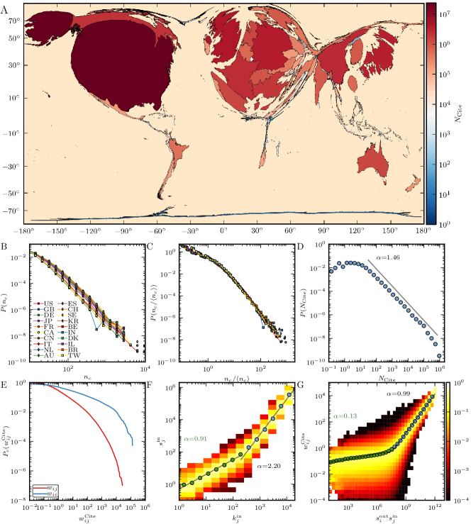
In order to find out the quality of papers published by different countries we consider the number of citations of each of the papers written by that country. In Fig. 1B we plot the probability distribution of the number of citations of papers in the largest 20 countries. A paper is associated to a country if at least one of its affiliations is from that country. All these distributions are broad and vary over four orders of magnitude. When each distribution is rescaled by the average number of citations of papers of the respective country, all curves nicely collapse (Fig. 1C). This result suggests that the functional form of the citation distribution is the same in each country and that the difference between countries can be effectively summarized by the average number of citations. This type of universality holds at the level of scientific disciplines as well Radicchi et al. (2008).

Next we consider the contribution at the level of cities. In Fig. 1D we plot the probability distribution of the cities’ citations. The distribution is broad, spanning over five orders of magnitude, and it follows a power law decay with exponent $1.46\pm 0.03$. This suggests a relationship with the population of the city, as the city size distribution obeys the Zipf law Zipf (1949); Gabaix (1999), i.e. decays as a power law (with exponent $2$). The observed power law scaling relation might suggest a self-organization phenomena due to the agglomeration benefits in science. These advantages can be due to the ease in collaboration between groups working in similar fields, sharing of infrastructure and support, etc., which leads to efficient integration and transfer of information.

We now consider the weighted citation network between cities, where the nodes are the cities that are connected by weighted and directed links, indicating publications of one city citing publications of the others. The network has 18,199 nodes and 9,494,021 links including 14,447 self-links (i.e., citations within the same city). In Fig. 1D we plot the cumulative distribution of the weights of self-links and links between different nodes. Both these distributions are broad; however, the weights of self-links are more heterogeneous, revealing a bias towards self-citations. Next we calculate the number of incoming links, i.e., the in-degree $k_{i}^{\mathrm{in}}$ of each node $i$ and its in-strength, $s_{i}^{\mathrm{in}}=\sum_{j}w_{ji}^{\mathrm{Cite}}$, which equals the number $N_{i}^{\mathrm{Cite}}$ of (normalized) citations received. By plotting the in-degree against the in-strength, we find that there is a power law scaling behavior with $\langle s^{\mathrm{in}}\rangle(k^{\mathrm{in}})\propto(k^{\mathrm{in}})^{\alpha}$ (Fig. 1E). However, there are two distinct scaling regimes: for nodes with small $k_{i}^{\mathrm{in}}$ ($<200$) the exponent is $\alpha=0.91\pm 0.03$ (regression coefficient $\pm$ standard error of the estimate $R=0.95\pm 0.01$), while for large $k_{i}^{\mathrm{in}}$ ($\geq 200$) the exponent is $\alpha=2.20\pm 0.08$ ($R=2.01\pm 0.01$). The super-linear behavior suggests that stronger links are more frequently connected to high in-degree nodes. The out-strength of the nodes follows a similar relationship with the out-degree of the nodes (see Appendix Fig. B.1). Finally, we plot the weights of the links $w_{ij}^{\mathrm{Cite}}$ against the product of the node strength $s_{i}^{\mathrm{out}}s_{j}^{\mathrm{in}}$. The product $s_{i}^{\mathrm{out}}s_{j}^{\mathrm{in}}$ gives the weight of a link that is expected to occur by chance between $i$ and $j$ if all the papers would be citing each other at random. Even in this case there are two distinct scaling regions, $w_{ij}^{\mathrm{Cite}}\propto(s_{i}^{\mathrm{out}}s_{j}^{\mathrm{in}})^{\alpha}$, where $\alpha=0.13\pm 0.01$ ($R=0.19\pm 0.0003$) if the product is less than $2\times 10^{7}$, while for larger values of the product $\alpha=0.99\pm 0.01$ ($R=1.07\pm 0.001$). This suggests that the observed citation is as expected between high strength nodes, while it is much lower in case of cities with low strength.

Figure 2: Properties of the world collaboration network. (A) Cumulative probability distribution of the link weights in the collaboration network of cities. Self-links are shown separately. (B) Fraction of internal collaboration, indicated by the ratio of the weight $w_{ii}^{\mathrm{Col}}$ of the self-link and strength $s_{i}$ of a node, against $s_{i}$. (C) Strength of a node against its degree. The straight line indicates a power law behavior with exponent $1.66\pm 0.04$. In these plots we use the same colorbar as in Fig. 1.

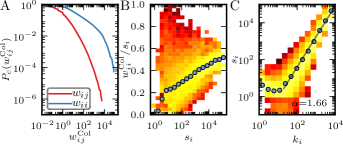
Let us now consider the collaboration network at the city level, where the nodes are cities and weighted undirected links indicate the presence and frequency of collaborations between scholars of different cities. There are 18,199 nodes in the network and 1,256,718 undirected links including 14,954 self-links. The weight of the self-links indicates the amount of internal collaboration. The degree of a node $i$ indicates the number of other cities with which $i$ collaborates and its strength is indicative of, but not coincident with, the number of papers written by scholars of institutions in that city.

In Fig. 2A we plot the cumulative probability distribution of link weights. As for citations, the weights of self-links are more broadly distributed than the weights of the links between different cities, showing that scholars of a city collaborate more frequently with each other than with colleagues from any other city. The distributions of collaboration and citation streams between cities differ from their analogues in mobile phone communications and world trade, that show log-normal distributions Krings et al. (2009); Bhattacharya et al. (2008). Next, we consider the fraction of internal collaboration by calculating the ratio of the weight of the self-link to the strength of the node. By plotting $w_{ii}^{\mathrm{Col}}/s_{i}$ against the strength of the node $s_{i}$, we see that the ratio increases with $s_{i}$, indicating that as the city size increases most of its collaborations take place within the city (Fig. 2B). However, for small cities most of their papers are written with external collaborators. The node degree scales with its strength as $\langle s\rangle(k)\propto k^{\alpha}$, where $\alpha=1.66\pm 0.04$ ($R=1.65\pm 0.01$) (Fig. 2C). This super-linear scaling suggests that higher degree nodes are more frequently connected by stronger links.

Figure 3: Correlation between the world citation and collaboration networks. Weight of the links in the citation network against the corresponding links in the collaboration network at the (A) country level and (B) city level network. Power law scaling is shown by solid lines with exponents $1.04\pm 0.01$ and $0.82\pm 0.02$, respectively. Density plot of the number of citations of a publication against the number of (C) co-authors, (D) countries (E) cities in the affiliation. The circles indicate the average trend.

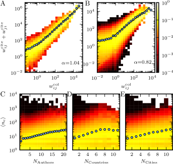
Let us explore the relationship between the citation and the collaboration networks at both the country and the city level. At the country level the collaboration network comprises 226 nodes and 10,308 undirected links, including 219 self-links. In the citation network there are also 226 nodes but 28,869 directed links, including 215 self-links. In Fig. 3, we plot the weight of links of the collaboration network, $w_{ij}^{\mathrm{Col}}$ against the weight of the same links in the citation network, $w_{ij}^{\mathrm{Cite}}+w_{ji}^{\mathrm{Cite}}$. We find scaling $w_{ij}^{\mathrm{Col}}\propto(w_{ij}^{\mathrm{Cite}}+w_{ji}^{\mathrm{Cite}})^{\alpha}$ where $\alpha=1.04\pm 0.01$ ($R=1.08\pm 0.008$) for countries (Fig. 3A), and $\alpha=0.82\pm 0.02$ ($R=1.05\pm 0.002$) for cities (Fig. 3B), i.e. the increase in collaboration is linearly related to the amount of citations exchanged between the two countries/cities.

Table 1: Dependence of citations on collaboration. We categorize each paper by the number of authors and their affiliations. For each of these groups we indicate the fraction of papers that are in the group and the mean number of citations. The error represents the standard error of the mean, calculated using bootstrap sampling with repetition.

$N_{\mathrm{Authors}}$	$f_{\mathrm{Papers}}$	Single	Multiple	Multiple
	(in %)	City	City	Countries
1	13.03	4.25 $\pm$ 0.02	4.95 $\pm$ 0.12	5.24 $\pm$ 0.11
2	19.01	6.80 $\pm$ 0.02	6.11 $\pm$ 0.04	7.00 $\pm$ 0.05
3	18.34	6.92 $\pm$ 0.02	6.38 $\pm$ 0.03	7.30 $\pm$ 0.04
4	14.95	7.19 $\pm$ 0.02	7.02 $\pm$ 0.03	8.03 $\pm$ 0.04
5	11.10	7.62 $\pm$ 0.03	7.66 $\pm$ 0.03	8.79 $\pm$ 0.04
6	8.01	8.13 $\pm$ 0.04	8.52 $\pm$ 0.05	9.77 $\pm$ 0.05
7	5.20	8.85 $\pm$ 0.05	9.56 $\pm$ 0.07	10.90 $\pm$ 0.07
8	3.45	9.50 $\pm$ 0.07	10.67 $\pm$ 0.09	12.10 $\pm$ 0.10
9	2.22	10.23 $\pm$ 0.10	11.52 $\pm$ 0.12	13.17 $\pm$ 0.12
10	1.53	10.57 $\pm$ 0.12	12.45 $\pm$ 0.14	14.70 $\pm$ 0.15
$>$10	3.17	13.82 $\pm$ 0.17	16.64 $\pm$ 0.16	21.37 $\pm$ 0.17

We now consider the dependence of the number of citations of a paper on the number of coauthors of that paper and on the number of affiliations of its coauthors. It has been previously shown that papers published by teams often get more citations than single author papers Wuchty et al. (2007); Jones et al. (2008). Our results also show that the average number of cites of a publication increases with the number of co-authors of that publication (Fig. 3C). Furthermore, the average number of citations of a publication increases with the number of affiliated countries and cities of its authors (Fig. 3D and E). In order to separate the effect of the number of coauthors and different type of collaboration (internal, domestic and international) we grouped each paper based on its affiliations and number of coauthors. In Table 1, we consider papers with a given number of authors and categorize them according to whether all the affiliations listed in the paper are from a single city, from multiple cities in a single country or from different countries. For an equal number of authors, publications having multiple international affiliations get a statistically significant increment ($p<10^{-4}$) in the number of citations with respect to publications with only domestic affiliations. Thus, crossing territorial boundaries also pays off in terms of scientific impact. In contrast, multiple domestic affiliation do not positively effect the number of citations when the number of authors in a publication is less than $6$.

Figure 4: Effect of geographical proximity in the world collaboration and citation networks. The probability of existence of a link as a function of the distance between two cities in the (A) collaboration network and (B) citation network. Distribution of the ratio of the link weight and product of the strengths of its endpoints in (C) collaboration network, $w_{ij}^{\mathrm{Col}}/s_{i}s_{j}$ and (D) citation network, $w_{ij}^{\mathrm{Cite}}/s_{i}^{\mathrm{out}}s_{j}^{\mathrm{in}}$ against the distance $d_{ij}$ between the cities. For each distance the average ratio is also shown. The solid line indicates a power law behavior with exponent $\alpha=1.16\pm 0.03$ and $0.77\pm 0.02$ respectively.

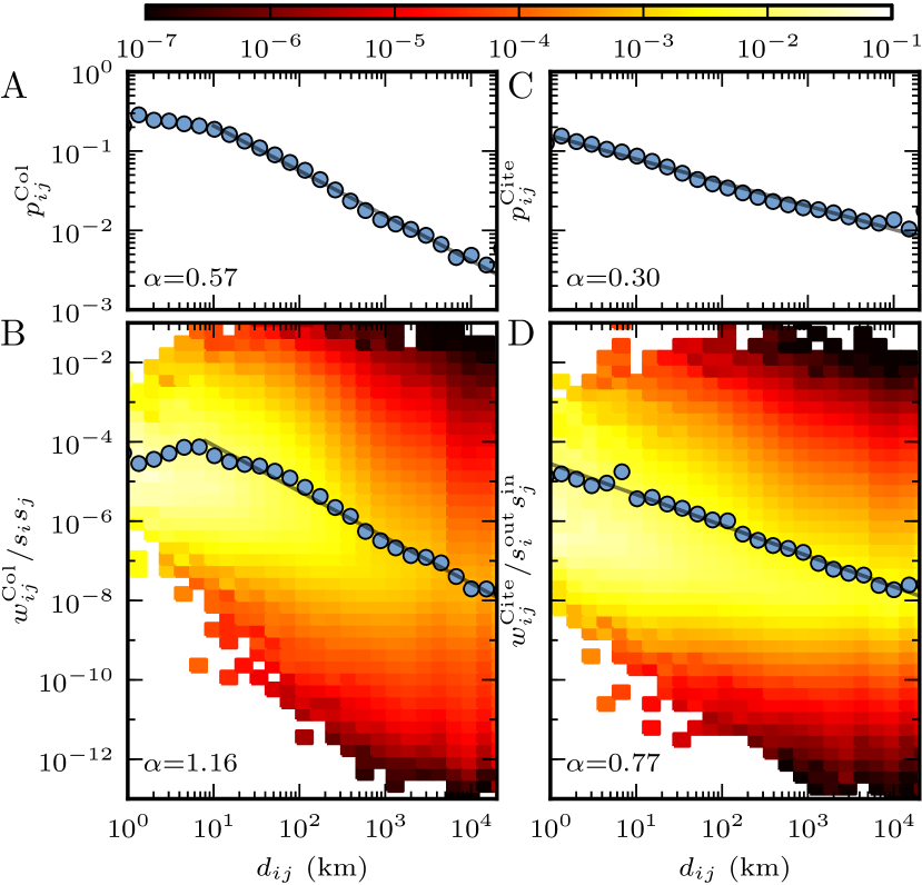
Next we consider the effect of geographical proximity on the citation and collaboration networks by determining the geographic location (latitude and longitude) of each place in the dataset Barthélemy (2011) (see Methods). We found that the probability that there is a link between two cities in the collaboration network decreases as a power law as the distance between the two cities increases (Fig. 4A). The power law exponent is $0.57\pm 0.01$. Our results are different from those obtained in Ref Katz (1994), where it was found that the distribution of distances between co-authors decreases exponentially. Such difference might be due to the limited dataset used in Ref Katz (1994), which included only papers published before 1990, and possibly also due to the recent advances in communication and transportation technologies.

Many spatially embedded networks have been observed to follow gravity laws Barthélemy (2011), where the flow between two locations follows

$$T_{ij}\propto\frac{P_{i}P_{j}}{d_{ij}^{\alpha}}.$$ (1)

Here, $T_{ij}$ is the flow between nodes $i$ and $j$, $P_{i}$ and $P_{j}$ are the populations of nodes $i$ and $j$, respectively and $d_{ij}$ is the geodesic distance between $i$ and $j$, the value of exponent $\alpha$ being dependent of the system. For the collaboration network Eq. 1 becomes

$$w_{ij}^{\mathrm{Col}}\propto\frac{s_{i}s_{j}}{d_{ij}^{\alpha}}.$$ (2)

In Fig. 4B, we plot the ratio ${w_{ij}^{\mathrm{Col}}}/({s_{i}s_{j}})$ against the distance $d_{ij}$ between all node pairs. We found that as the distance increases $\langle{w_{ij}^{\mathrm{Col}}}/({s_{i}s_{j}})\rangle$ decreases as a power law with the exponent $\alpha=1.16\pm 0.03$ ($R=-0.97\pm 0.002$), except at very short distances. As we have seen before, collaboration and citation between two places are correlated. Hence, we also look at the geographical proximity in the citation network. We found that the probability that there is a link between two cities in the citation network also decreases with distance as a power law (Fig. 4C). In this case the power law exponent is much lower ($0.30\pm 0.01$). The gravity law for the citation network reads

$$w_{ij}^{\mathrm{Cite}}\propto\frac{s_{i}^{\mathrm{out}}s_{j}^{\mathrm{in}}}{d_{ij}^{\alpha}}.$$ (3)

In Fig. 4D we plot ${w_{ij}^{\mathrm{Cite}}}/({s_{i}^{\mathrm{out}}s_{j}^{\mathrm{in}}})$ against the distance between all the node pairs in the citation network. As for the collaboration network we found that $\langle{w_{ij}^{\mathrm{Cite}}}/({s_{i}^{\mathrm{out}}s_{j}^{\mathrm{in}}})\rangle$ decreases with distance as a power law with the exponent $\alpha=0.77\pm 0.02$ ($R=-0.35\pm 0.001$). The above analysis shows the existence of an important spatial component in both the citation and the collaboration network. It shows that both our collaborators and our citations typically come from our spatial neighborhood. Further, long distance collaborations as well as citations decrease as a power law of distance. The difference of the scaling exponents of the two networks suggests that two distant places are more likely to cite each other than collaborate. Additional results are shown in the Appendix Fig. B.3.

Figure 5: Relation between research outcome and funding. Average number of citations per paper of a country against (A) the expenditure in research and development (in millions of dollars per year, and purchasing power parity) and (B) the number of researchers in that country. The solid line indicates power law scaling with exponent $0.99\pm 0.03$ and $0.98\pm 0.04$, respectively. (C) Average number of citations per paper of a country against the average spending per researcher. The horizontal line indicates the average number of citations over all papers of all countries, the vertical line indicates the threshold of about 100,000 $ per researcher per year.

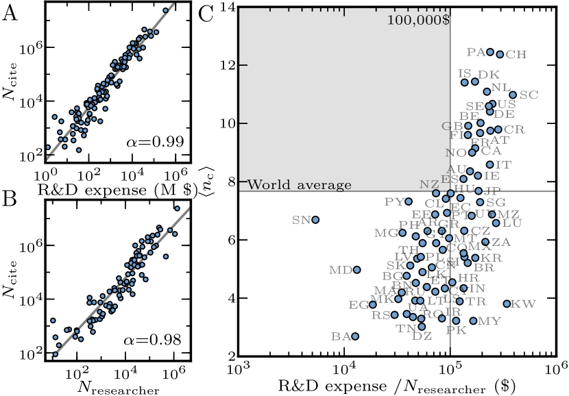
The research performance of each country is generally estimated on the basis of the number of publications and citations. Although these are straightforward measurements of research output, they depend on a wide spectrum of resources Johnes and Johnes (1995). For instance, the number of researchers and facilities (instruments, laboratories, libraries and other resources) available are typically different in different countries. A key determinant is the funding available for research & development (R&D). To quantify the expenses in R&D of a country we consider the fraction of gross domestic product (GDP) that is spent on R&D. To get rid of economic inequalities in different countries we consider the R&D spending in terms of the purchasing power parity (PPP). In Fig. 5A, we plot the number of citations $N_{\mathrm{Cite}}$ against the R&D expenditure and find that it scales linearly with funding. Such correlation is not surprising, but the scaling exponent is non-trivial. It suggests that it is not possible to perform or contribute substantially unless there is a corresponding amount of funding available for research. Moreover, the research contribution in terms of citations also scales linearly with the number of researchers in that country (Fig. 5B). This result is consistent with the fact that the R&D expenditure is correlated with the number of researchers. The number of publications of a country also shows similar scaling against R&D expenditure and number of researchers (Appendix Fig. B.4).

Finally as a measure of impact of a country’s scientific output we consider the average number of citations to the publications of that country. In Fig. 5C we plot this number against the average spending per researcher per year (R&D expenditure divided by the number of researchers). The latter is not the average salary of researchers in that country, as it includes other expenditures such as infrastructure, bureaucracy, instruments, etc. This plot is much more scattered than the previous plots and does not show any definite correlation pattern. In order to identify groups of countries that behave similarly or show similar characteristics we use the $k$-mean clustering technique Sculley (2010). By using this clustering method with $k=2$, we found that the countries can be classified into two groups, one with average spending less than about 100,000 $ per researcher per year and other with average spending more than about 100,000 $ (Fig. S5). Another clustering methods also give qualitatively similar results. This separation in two groups, distinguished by the average spending per researcher per year (vertical line in the plot) also reveals another striking feature. If the average spending is less than about 100,000 $ (vertical line in the plot) per researcher per year we see an increase in the average number of citations with the spending. However if the average spending exceeds this limit, it becomes scattered and independent of funding. This figure shows that very rich countries like Kuwait and Luxembourg have high funding per researcher, still the average number of citations per paper is low. Countries like India, Brazil have high funding per researcher as well, but low average number of cites; this might mean they are investing more on infrastructure. Switzerland, Costa Rica, Panama, Germany, Austria, Netherlands, United States have high spending per researcher and their average number of citations is also high. If we display the number of cites per paper averaged over all countries (horizontal line), we see that there are no countries in the top left quadrant, i.e. it is not possible to do better than the world’s average unless there is sufficient spending. Additional measures of a country’s research performance and corresponding rankings are reported in the Appendix Table LABEL:tab:contribution.

III Discussion

Our thorough analysis of the world citation and collaboration networks has revealed that the effects of geography on the dynamics of science are relevant, despite the recent advances in communication and transportation. The occurrence of gravity laws for both citation and collaboration implies a preference by scientists to interact with peers in their geographic areas. However, long-distance interactions are not rare, as the interaction strength and probability are characterized by power law decays. Our work follows similar findings in mobile phone communication Lambiotte et al. (2008); Krings et al. (2009), social media Liben-Nowell et al. (2005) and international trade Kaluza et al. (2010), reinforcing the belief that gravity laws hold in several different contexts, and that scientific interactions are not exceptional from this point of view. Thus, the gravity law is a fundamental relationship holding also in human dynamics.

Citation and collaboration streams between distinct locations are strongly correlated, with an approximately linear relation. An increase in the number of collaborations between two cities is then expected to be followed by a proportional increase in the flow of citations between the cities. This is justified from the fact the people/groups working in similar fields and subject area are more likely to cite as well as collaborate with each other, and also suggests a natural bias towards self-citation, of which we have provided strong quantitative evidence.

From the point of view of scientific impact, it pays off for a team to put together several institutions with a strong international participation. While part of this effect could be justified by the fact that having people from different locations facilitates the circulation of a work, which then becomes more visible and susceptible to be cited, the trend indicates that it is more likely to produce high quality work through international collaborations. It would be valuable to be able to disentangle the impact due to social networking from that due to the quality of the paper. Our findings pave the way for the first quantitative assessment of this issue. As a consequence, we expect to observe an increasing tendency to form large teams with members of many different countries in the future.

We also disclose a striking effect in the relationship between the national expenditure per researcher and the impact of the scientific output of a country. If the average spending per researcher per year is low, it is impossible for a country to do better than the world average, in terms of the average number of cites per paper. So there is a minimal funding quota that needs to be exceeded if a country wishes to have a scientific output of high average quality. Exceeding the threshold, however, does not guarantee success. This suggest that in science money acts as a kind of threshold motivator: if one does not pay people enough they will not be motivated and the outcomes of the research are poor; if people are paid sufficiently to take the issue of money off the table, internationally competitive findings are within reach. On the other hand, for conceptual and creative tasks, paying more than a certain threshold does not necessarily increase the output Adams (1966); Alderfer (1972); Deci and Ryan (1985). Further, our analysis reveals that at the country level funding has a positive linear impact on the research output both in terms of number of publications as well as citations. Thus, it is not possible for a country to increase its research output substantially without a sizeable increase in investments.

In the future we plan to study the role of cities’ population, in particular on the distributions of citation and collaboration strengths along with their flows. It is well known that most characteristics of cities are strongly correlated to the size of their populations Bettencourt et al. (2007). Furthermore, an analysis of the evolution of the world citation and collaboration networks would show how the spatial dimension of science dynamics has been affected by the progress of technology, internationalization and extreme events (e.g. wars, economic crises). This way one could infer how the scientific landscape has been shaping up in the last decades and how is it possible to create more efficient partnerships, via dedicated funding programs at the national and/or international level, and consequently a more productive and successful scholarly world.

IV Methods

IV.1 Data description

We have analyzed all publications (articles, reviews and editorial comments) written in English from 2003 till the end of 2010 included in the database of the Institute for Scientific Information (ISI) Web of Science. For each publication we extract the affiliations of the authors and the corresponding citations to that publication. We parsed the affiliations of all publications and have determined the geographic location at the city and country level. If there are multiple affiliations listed in a publication, the latter is associated with all represented cities and countries. After obtaining the locations we use the publicly available resources (www.wikipedia.org and maps.google.com) to determine their coordinates (latitude and longitude). Our dataset consists of 8,094,948 publications which have received 62,105,592 citations during the period 2003-2010. We were able to extract the geographical information from 8,092,314 publications. Affiliations refer to 226 countries and 37,750 cities. In order to get rid of anomalies due to any misclassification, we have only consider those places that have appeared in at least 5 publications during the period 2003-2010. This cutoff led us to 18,199 cities, producing 99.8% of the total publications and receiving 99.9% of total citations.

Country level information regarding expenditures for research and development (R&D) in terms of purchasing power parity (PPP) and number of researchers in R&D are obtained from the World Bank Data (databank.worldbank.org) for each year between 2003 till 2010. By aggregating these yearly datasets we determine the average of each of the above quantities for the period 2003-2010. The data of expenditure for R&D is available for 102 countries, the numbers of researchers for 89 countries and for 77 countries both informations are available. Further details can be found in the Appendix.

IV.2 Network construction

We have analyzed the data at the country and the city level. As the publications and their affiliations form a bipartite graph, we construct the collaboration network between countries (cities) by projecting it onto the space of affiliations. In this collaboration network individual countries (cities) act as nodes, and links between them indicate that they have appeared in the same publication. If a paper is written by authors with $n$ affiliations, we put $\frac{1}{2}n\times(n-1)$ undirected links between each possible pair of collaborating countries (cities), with every link having weight $\frac{2}{n\times(n-1)}$. The total weight between any pair of nodes is the sum of all the weights over all the publications in the dataset. If there is a single affiliation in a publication then we put a self-link with weight 1.

In the citation network between countries (cities) nodes are papers which are linked if one paper cites the other. If a paper written by authors with $n$ affiliations cites a paper written by authors with $m$ affiliations we put $n\times m$ directed connections from each of the $n$ citing countries (cities) to each of the $m$ cited countries (cities), every link having weight $1/(nm)$. The total weight of a directed link between two countries (cities) is the sum of all the weights over all the citations in the dataset. Since there can be multiple affiliations from the same country (city) in a publication, there are self-loops both in the world citation and in the world collaboration networks.

IV.3 Great-circle distance

The geodesic or the great-circle distance is the shortest distance between any two points on the earth measured along a path on the surface of the earth. Given the latitudes and longitudes of two points, we have used the Haversine formula to calculate the great-circle distance between them Sinnott (1984). In these calculations, we considered the earth’s radius to be 6372.8 KM.

Appendix A Materials and methods

A.1 Data description

For our study we used all publications in English in the databases of Science Citation Index Expanded, Social Sciences Citation Index, and Arts & Humanities Citation Index for the years 2003-2010. The database of the Institute for Scientific Information (ISI) Web of Science also includes publications in other major languages, but consists of a relatively small number of items, accounting for $<5\%$ of total publications. For each publication in the database, we have the name of the journal in which it is published, the volume and page number of the publication, its year of publication, the names of the authors, the list of their affiliations and its references and other additional information. We used the list of references to construct the network of citations between papers. For each publication we extracted the city and country of authors’ institutions from the affiliation data. Whenever a publication has several authors, it is counted and assigned to each location. Note that we only have the list of authors and the list of affiliations for each paper, however there is no corresponding match between these two lists and hence the individual level author affiliation can not be used in our study. Further although the affiliations are being recorded with increasing consistency, their use still poses major challenges in uniquely and accurately identifying them. For this reason, we parsed the affiliations of all publications and have determined the geographic location only at the city and country level. We also we use the publicly available resources (www.wikipedia.org and maps.google.com) to disambiguate the names of the places in case there are multiple name variation, typos and name changes during the time period of study.

A.2 GDP

The gross domestic product (GDP) is the value of all final goods and services produced within a nation in a given year and is the primary indicators used to gauge the health and size of a country’s economy. We consider the average GDP (in US dollars) of a country during 2003-2010. A nation’s GDP at purchasing power parity (PPP) exchange rates is the sum value of all goods and services produced in the country valued at prices prevailing in the United States. This is the measure most economists prefer when looking at per-capita welfare and when comparing living conditions or use of resources across countries.

A.3 R&D spending

Expenditures for research and development are current and capital expenditures (both public and private) on creative work undertaken systematically to increase knowledge, including knowledge of humanity, culture, and society, and the use of knowledge for new applications. R&D covers basic research, applied research, and experimental development.

A.4 Number of researcher

Researchers in R&D are professionals engaged in the conception or creation of new knowledge, products, processes, methods, or systems and in the management of the projects concerned. Postgraduate PhD students engaged in R&D are included.

A.5 Statistics

To fit the data and calculate different estimates we use the following methods:

Estimation of standard errors. Bootstrapping is a distribution-free re-sampling method used to estimate the parameters of interest from the empirical data. We have used this method in order to calculate the standard error of the mean. Let $x_{1},x_{2},\dots,x_{n}$ be the dataset with mean $\bar{x}$. The standard error is then calculated as follows Efron and Tibshirani (1993): (i) Draw $N$ samples each of size $n$ with replacement from the original data. (ii) For each of the $N$ samples calculate the sample mean $\hat{x_{1}},...,\hat{x_{N}}$ (iii) The standard error is then given by, $SEE(\bar{x})=\sqrt{\frac{1}{N-1}\sum_{i=1}^{N}(\hat{x_{i}}-\bar{\hat{x_{i}}})^{2}},$ where $\bar{\hat{x_{i}}}=N^{-1}\sum_{i}^{N}\hat{x_{i}}$ is the mean of the $N$ bootstrap sample. In this study we have used $10^{4}$ bootstrapped samples, i.e., $N=10^{4}$.

Estimation of significance difference. The above bootstrapping procedure however does not tell whether the difference in the means of two distributions is significant or not. In this case the re-sampling has to be performed according to an appropriate null hypothesis, whereas for standard errors the re-sampling procedure was unrestricted.

Let us consider two independent samples $x_{1},\dots,x_{n}$ and $y_{1},\dots,y_{m}$, and suppose that we are interested in the difference in the population means, $\delta=\bar{x}-\bar{y}$. Consider that the null hypothesis is $H_{0}:\bar{x}-\bar{y}=0$. We create the bootstrap sample by choosing $n$ elements without replacement from the pooled set $x_{1},\dots,x_{n},y_{1},\dots,y_{m}$. The remaining $m$ elements constitute the other sample. We then calculate the mean of both these samples and determine the difference between them, say $\hat{\delta}_{i}=\bar{\hat{x}}_{i}-\bar{\hat{y}}_{i}$. In analogous fashion $N$ re-samples are made, and the bootstrap $p$ value is defined as $p=\frac{(\#(\hat{\delta}_{i}\geq\delta,\leavevmode\nobreak\ \forall i))+1}{N+1}$. In this study we have used $10^{4}-1$ bootstrapped samples.

Power-law exponent. We use maximum likelihood techniques to estimate the scaling exponent of power law distributions Clauset et al. (2009).

Regression Coefficient. We used the linear regression analysis to study the relationship between the corresponding variables. We determine the regression coefficient using the ordinary least squares. The error term of the regression coefficient represents the standard error of the estimate.

A.6 Map construction

Statistical data with embedded geographical information can be visualized with standard maps which are color coded by region. However these maps are sometimes hard to interpret as the statistical measures are often correlated with the other indicators. We have used a diffusion-based method to create different density-equalizing maps Gastner and Newman (2004). In this method we start with an inhomogeneous distribution of the research contribution (in terms of citations, say) and let the diffusion process evolve until a homogeneous equilibrium state is reached: the displacements are then reinterpreted to generate the cartogram.

Appendix B Results

Figure B.1: Research contribution in terms of number of publications. (A) Map of the country’s research contribution, where the area of each country is scaled and deformed according to its number of publications. (B) The probability distribution function of the research contribution of cities in terms of their number of publications. The dashed line shows a power law scaling behavior with exponent $1.45\pm 0.01$. (C) Node out-strength against its out-degree for city citation network. There are two distinct power law scaling regions, with scaling exponents $0.82\pm 0.04$ and $2.26\pm 0.07$ for low and high degree ($>200$) nodes, respectively.

Figure B.2: (A) Average number of citations of each country. World map where countries are color coded based on the average number of citations per publication. Most countries stay below the world’s average of 7.67.(B) Weight of the links against the product of the strengths of the endpoints in the collaboration network of cities. There are two different scaling regions ($2\times 10^{7}$), with exponents $0.16\pm 0.01$ and $0.92\pm 0.03$.

We consider the research contribution of each country in terms of the number of publications $N_{\mathrm{Pub}}$, normalized by the number of participating countries in that publication. To visualize the results, we create a cartogram in which the geographic regions are deformed and rescaled in proportion to their relative research contribution Gastner and Newman (2004). We observed that the contribution of different countries in terms of publications is heterogeneous and varies over 6 order of magnitude. Fig. B.1A shows that North America (32.4%), Europe(33.7%) and Asia(27.4%) have prominent contribution in terms of the number of publications. On the other hand, Africa, South America and Oceania contribute less than 7% of world’s publications. Table. LABEL:tab:contribution shows the contribution, number of countries and cities in each continents. It also indicates the statistics of the top countries of each continent. It is evident that the United States are the leading country in the world both in terms of publications and citations to them. It is followed by China, United Kingdom, Japan, and Germany in terms of publications, whereas in terms of citations it is followed by United Kingdom, Germany, Japan, and China. We indicate the fraction of total publications $f_{\mathrm{Pub}}$, the fraction of total citations received $f_{\mathrm{Cite}}$ and the average number of citations per paper, for countries that received more than 0.005% of world citations. Countries are listed in decreasing order of the fraction of total citations received. The superscripts in $f_{\mathrm{Pub}}$ and $f_{\mathrm{Cite}}$ indicate the world ranking of that country according to the numbers of publications and citations, respectively. We then consider the contribution in terms of the number of publications at the level of cities. In Fig. B.1B we plot the probability distribution of the cities’ contributions in terms of their publications and observed that it follows a power law scaling behavior with exponent $1.45\pm 0.01$. By plotting the out-degree against the out-strength, we find that there is power law scaling behavior with $\langle s^{\mathrm{out}}\rangle(k^{\mathrm{out}})\propto(k^{\mathrm{out}})^{\alpha}$ (Fig. B.1C). However, there are two distinct scaling regimes: for nodes with small $k_{i}^{\mathrm{in}}$ ($<200$) the exponent is $\alpha=0.82\pm 04$, while for large $k_{i}^{\mathrm{out}}$ ($\geq 200$) the exponent is $\alpha=2.26\pm 0.07$. The super-linear behavior suggests that stronger links are more frequently connected to high out-degree nodes.

Figure B.3: Gravity law in the world collaboration and citation networks.(A) Variation of the probability of existence of a link between two nodes as a function of the product of their strengths in the (A) collaboration network and (B) citation network of cities. Variation of the average link weight against the distance between the cities in the (C) collaboration network and (D) citation network. For each distance the average ratio is also shown. In this case only the existing links are considered while calculating the averages. The solid line indicates a power law behavior with exponent $\alpha=0.31\pm 0.01$ and $0.22\pm 0.01$ respectively. Variation of the average link weight against the distance between the cities in the (E) collaboration network and (F) citation network. For each distance the average ratio is also shown. In this case all possible node pairs are considered in order to calculate the average, i.e., links that do not exist are considered with weight 0. The solid line indicates a power law behavior with exponent $\alpha=0.88\pm 0.02$ and $0.51\pm 0.02$, respectively.

Figure B.4: Relation between research contribution in terms of number of publications and funding. Country’s number of publications against the (A) expenditure in research and development (in million dollars, and purchasing power parity), (B) number of researchers in that country. The solid line indicates a scaling with exponent $0.90\pm 0.03$ and $0.96\pm 0.03$, respectively. (C) The plot of average spending per researcher against the average number of citation per paper of that country. The average number of citations is now defined as the ratio of the normalized number of citations and normalized number of publications (see text). The horizontal line indicates world average, the vertical line indicates the spending of 120 000 $ per researcher.

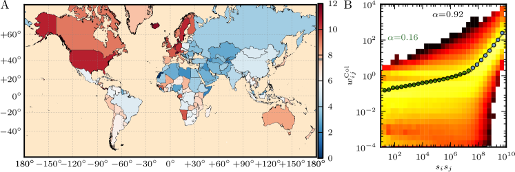
Next we consider the average number of citations per paper of each country and plot it on a colorpleth map (Fig. B.2A). For calculating the average citation of a country we consider all its publications and count the total number of citations to all these articles during the period of 2003-2010. In the case where a publication has multiple affiliations from different countries, it is counted multiple times for the countries’ averages, once for each of the affiliated countries. In Table LABEL:tab:contribution, we have also given the average number of citations per paper of the top countries in each continent. The world average is 7.67. United States, Canada, Australia and most of the European countries have average number of citations larger than the world average. In Europe Switzerland leads the table, followed by Denmark and Netherlands. In contrast most of the countries from Asia stay below the world average, the only exception being Israel. Most of the countries in Africa and South America are below the world average as well. Other notable countries are Bermuda (16.97$\pm$5.95), Gambia (16.17$\pm$3.10), Panama (12.41$\pm$ 0.68), Iceland (11.43$\pm$ 0.71), Seychelles (11.11$\pm$ 2.40), Guinea-Bissau (10.10$\pm$ 0.97), Costa Rica (9.82$\pm$ 0.93), and Austria (9.75$\pm$ 0.09). For the collaboration network of cities we plot the weight of the links against the product of the strengths of the connecting nodes, expressing the expected weight of random collaborations (Fig. B.2B). As for citations we find that $w_{ij}^{\mathrm{Col}}\propto(s_{i}s_{j})^{\alpha}$, with two different scaling exponents. If $s_{i}s_{j}<2\times 10^{7}$, $\alpha=0.16\pm 0.01$ ($R=0.11$), whereas if $s_{i}s_{j}>2\times 10^{7}$ $\alpha=0.92\pm 0.03$ ($R=1.18$).

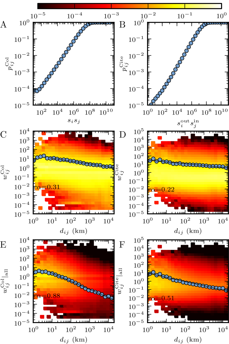
In Fig. B.3A,B we plot the probability of existence of a link as a function of the product of strength of the end-points of the link. We found that as the product increases, both in the collaboration and the citation network the probability of link existence increases, as expected. In Fig. B.3C,D we show the variation of the link weight against the distance between the end-points. We found that both in the collaboration and the citation network on the average the link weight decreases as a power-law with exponent $0.31\pm 0.01$ and $0.22\pm 0.01$, respectively. In this figure, while calculating the averages we have only considered the existing links between nodes. However, in the main text we have seen that the probability of link existence also decreases with distance. If we take this information while calculating the averages, i.e., we consider the non-existent links by assigning weight zero to them, we found that in both the collaboration and the citation network, the average link weight decreases with distance as a power law, with exponent $0.88\pm 0.01$ and $0.51\pm 0.01$, respectively (Fig. B.3E,F). Note that this property is different from what has been observed in the mobile phone communication network, where it was shown that the weight of the existing links are independent of the distance, whereas the overall link weight decrease as a result of decreasing probability of having a link as the distance increases Krings et al. (2009).

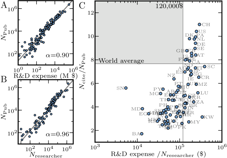
In the main paper we have considered the research performance of each country based on the number of citations. In addition, here we consider the performance of a country based on its number of publications. As before, in Fig. B.4A, we plot the research contribution in terms of the number of publications $N_{\mathrm{Pub}}$ against the countries’ R&D expenditure in terms of purchasing power parity (PPP). We found that this indicator also scale almost linearly with the spending. We next consider the dependence of research performance on the number of researchers in that country (Fig. B.4B). The research contribution in terms of publications also scale linearly with the number of researchers in that county.

Finally as a measure of the average publication quality of a country we consider the ratio of the normalized number of citations and normalized number of publications of that country. This is an alternative measure of the average number of citations per paper we mentioned above, which is not normalized by the number of authors in a paper. In the previous measure each publication from a country (independently of the number of participating countries) gets equal weight while calculating the average. In this other measure, if there are $n$ countries in a publication, each country would get $1/n$ as credit for that publication, so that publication would give a lower contribution to the average number of cites per paper than before. In Fig. B.4C we plot the new quantity against the average spending per researcher of the country (R&D expenditure divided by the number of researchers). Although this plot is similar to the one in the main paper, there are certain differences in the average number of citations of some countries. For example, Italy, Spain, Norway are now below the world average. This means that the publications from these countries with international collaborators contribute significantly to the average impact of their scientific production.

Figure B.5: Data clustering. (A) Decomposition obtained using $k$-mean clustering with $k=2$. (B) Decomposition obtained using mean shift clustering. Each cluster is indicated by a color.

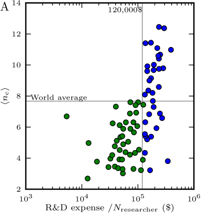
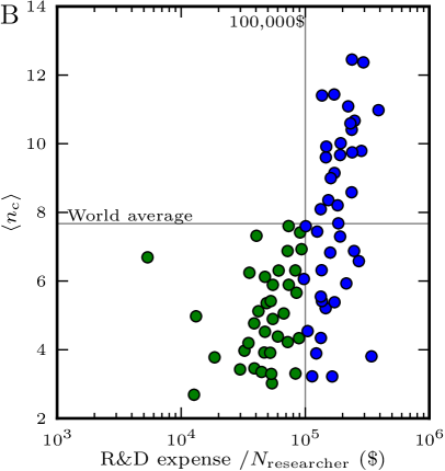
In order to check whether the countries in Fig. 5C can be categorized into different groups based on the average spending per researcher and the average number of citations, we used two different clustering methods. The $k$-means clustering technique Sculley (2010) partitions the data into $k$-mutually exclusive clusters. The aim here is to determine whether there are inherent clusters in Fig.5C and Fig B.4C. For the $k$-means clustering method we need to specify the number $k$ of clusters before starting the clustering process. The method consists in the minimization of an objective function expressing the sum of square distances between each data point and its centroid, i.e. a geometrical point whose position is also consistently determined by the minimization procedure: each centroid corresponds to one cluster. We can follow a procedure to minimize the objective function iteratively by finding a new set of cluster centroids that can lower the value of the objective function at each iteration. On using this method with $k=2$, we found that the countries can be classified into two groups, one with average spending less than about 120,000 $ per researcher per year and other with average spending more than about 120,000 $ (Fig. B.5). We also use a different method, the mean shift clustering algorithm Comaniciu and Meer (2002) to determine the clusters in the data in Fig.5. This is a nonparametric clustering technique and does not require prior knowledge of the number of clusters. The mean-shift algorithm seeks local maxima of density of points in the feature space. This method also detects two different clusters, one with average spending less than about 100,000 $ per researcher per year and the other with average spending more than about 100,000 $. Thus, these two methods give slightly different thresholds however the results are qualitatively similar.

Table B.1: Research contribution of different continents and their top countries. The number of countries and cities in each continent are indicated by $N_{\mathrm{Countries}}$ and $N_{\mathrm{Cities}}$, respectively. Fraction of publications $f_{\mathrm{Pub}}$, fraction of citations received $f_{\mathrm{Cite}}$ and the average number of citations per paper of each continent is also indicated. For top countries in each continent we list the fraction of publications $f_{\mathrm{Pub}}$, fraction of citations received $f_{\mathrm{Cite}}$, the average number of citations per paper. The superscript indicates the countries’ rank in the world in terms of number of publications and number of citations. Only countries that receive more than 0.005% of all citations are shown.

Continent	$N_{\mathrm{Countries}}$	$N_{\mathrm{Cities}}$	$f_{\mathrm{Pub}}$	$f_{\mathrm{Cite}}$	Avg. Cites	Country	$f_{\mathrm{Pub}}$	$f_{\mathrm{Cite}}$	Avg. Cites
			(in %)	(in %)		name	(in %)	(in %)
Africa	57	749	1.32	0.65	5.00$\pm$0.05	South Africa	$0.430^{33}$	$0.248^{37}$	5.92$\pm$0.08
						Egypt	$0.286^{38}$	$0.128^{40}$	3.78$\pm$0.05
						Tunisia	$0.100^{52}$	$0.036^{52}$	3.33$\pm$0.13
						Nigeria	$0.126^{50}$	$0.031^{56}$	2.82$\pm$0.25
						Kenya	$0.038^{65}$	$0.028^{58}$	7.55$\pm$0.29
						Morocco	$0.055^{60}$	$0.025^{60}$	4.20$\pm$0.10
						Algeria	$0.067^{54}$	$0.023^{62}$	3.01$\pm$0.08
						Tanzania	$0.019^{83}$	$0.014^{74}$	7.27$\pm$0.29
						Uganda	$0.018^{85}$	$0.014^{75}$	7.04$\pm$0.27
						Cameroon	$0.021^{77}$	$0.010^{80}$	4.72$\pm$0.18
						Ethiopia	$0.022^{75}$	$0.009^{81}$	4.36$\pm$0.17
						Ghana	$0.016^{86}$	$0.008^{85}$	5.29$\pm$0.21
						Zimbabwe	$0.011^{95}$	$0.007^{87}$	5.92$\pm$0.28
						Malawi	$0.009^{103}$	$0.006^{88}$	7.11$\pm$0.32
						Senegal	$0.008^{104}$	$0.006^{90}$	6.72$\pm$0.29
						Botswana	$0.010^{97}$	$0.005^{95}$	5.46$\pm$0.54
						Gambia	$0.003^{128}$	$0.005^{96}$	15.87$\pm$3.02
						Cote d’Ivoire	$0.006^{107}$	$0.005^{97}$	7.20$\pm$0.41
Asia	49	3853	27.36	17.71	5.58$\pm$0.01	Japan	$6.457^{4}$	$5.939^{4}$	7.68$\pm$0.03
						China	$7.216^{2}$	$4.304^{5}$	5.05$\pm$0.02
						South Korea	$2.509^{10}$	$1.582^{13}$	5.38$\pm$0.04
						India	$2.727^{9}$	$1.398^{15}$	4.35$\pm$0.03
						Taiwan	$1.671^{15}$	$1.037^{16}$	5.19$\pm$0.04
						Israel	$0.863^{22}$	$0.837^{20}$	8.86$\pm$0.10
						Turkey	$1.450^{17}$	$0.667^{22}$	3.89$\pm$0.03
						Russia	$1.875^{13}$	$0.622^{24}$	3.92$\pm$0.05
						Singapore	$0.521^{29}$	$0.461^{28}$	7.29$\pm$0.08
						Iran	$0.747^{23}$	$0.308^{31}$	3.31$\pm$0.03
						Thailand	$0.244^{41}$	$0.147^{38}$	5.88$\pm$0.17
						Malaysia	$0.195^{42}$	$0.069^{45}$	3.22$\pm$0.07
						Pakistan	$0.175^{44}$	$0.059^{48}$	3.23$\pm$0.07
						Saudi Arabia	$0.131^{49}$	$0.046^{50}$	3.12$\pm$0.07
Asia	49	3853	27.36	17.71	5.58$\pm$0.01	Jordan	$0.061^{58}$	$0.023^{61}$	3.27$\pm$0.11
						Vietnam	$0.037^{68}$	$0.020^{66}$	5.59$\pm$0.30
						Indonesia	$0.032^{70}$	$0.019^{67}$	5.73$\pm$0.23
						Kuwait	$0.044^{61}$	$0.018^{68}$	3.80$\pm$0.16
						Bangladesh	$0.041^{63}$	$0.018^{69}$	4.74$\pm$0.17
						Lebanon	$0.038^{66}$	$0.018^{70}$	4.47$\pm$0.13
						UAE	$0.041^{62}$	$0.018^{71}$	4.03$\pm$0.14
						Philippines	$0.035^{69}$	$0.017^{72}$	6.20$\pm$0.30
						Cyprus	$0.027^{73}$	$0.012^{76}$	4.31$\pm$0.15
						Sri Lanka	$0.022^{76}$	$0.011^{79}$	4.90$\pm$0.18
						Armenia	$0.026^{74}$	$0.009^{82}$	6.18$\pm$0.31
						Oman	$0.021^{79}$	$0.008^{86}$	3.50$\pm$0.14
						Georgia	$0.020^{82}$	$0.006^{89}$	3.94$\pm$0.20
						Nepal	$0.012^{92}$	$0.006^{91}$	5.36$\pm$0.29
						Uzbekistan	$0.020^{81}$	$0.006^{92}$	3.50$\pm$0.17
Europe	47	6625	33.69	35.25	9.29$\pm$0.01	United Kingdom	$6.509^{3}$	$7.453^{2}$	9.91$\pm$0.04
						Germany	$5.131^{5}$	$6.299^{3}$	10.41$\pm$0.04
						France	$3.611^{7}$	$4.034^{6}$	9.67$\pm$0.04
						Italy	$3.415^{8}$	$3.258^{8}$	8.59$\pm$0.04
						Netherlands	$1.829^{14}$	$2.331^{9}$	11.08$\pm$0.07
						Spain	$2.482^{11}$	$2.258^{11}$	8.09$\pm$0.05
						Switzerland	$1.114^{19}$	$1.600^{12}$	12.38$\pm$0.09
						Sweden	$1.227^{18}$	$1.436^{14}$	10.59$\pm$0.09
						Belgium	$0.923^{21}$	$1.004^{17}$	10.02$\pm$0.08
						Denmark	$0.655^{25}$	$0.838^{19}$	11.45$\pm$0.12
						Finland	$0.640^{26}$	$0.672^{21}$	9.59$\pm$0.10
						Austria	$0.595^{27}$	$0.653^{23}$	9.75$\pm$0.11
						Poland	$1.110^{20}$	$0.579^{25}$	5.43$\pm$0.05
						Norway	$0.506^{30}$	$0.483^{26}$	8.98$\pm$0.10
						Greece	$0.684^{24}$	$0.468^{27}$	6.30$\pm$0.06
						Portugal	$0.460^{32}$	$0.345^{30}$	6.93$\pm$0.08
						Czech Republic	$0.464^{31}$	$0.301^{32}$	6.31$\pm$0.08
						Ireland	$0.340^{36}$	$0.298^{33}$	8.20$\pm$0.16
						Hungary	$0.338^{37}$	$0.251^{36}$	7.61$\pm$0.13
						Slovenia	$0.171^{45}$	$0.096^{41}$	5.41$\pm$0.09
						Ukraine	$0.271^{40}$	$0.088^{42}$	3.46$\pm$0.07
						Romania	$0.274^{39}$	$0.079^{43}$	3.30$\pm$0.09
						Slovakia	$0.150^{48}$	$0.072^{44}$	5.12$\pm$0.12
						Croatia	$0.164^{47}$	$0.068^{46}$	4.53$\pm$0.12
						Serbia	$0.167^{46}$	$0.061^{47}$	3.42$\pm$0.07
						Bulgaria	$0.125^{51}$	$0.056^{49}$	4.76$\pm$0.09
						Estonia	$0.063^{57}$	$0.041^{51}$	6.91$\pm$0.21
						Lithuania	$0.095^{53}$	$0.035^{53}$	3.91$\pm$0.13
						Iceland	$0.030^{71}$	$0.031^{57}$	11.46$\pm$0.63
						Belarus	$0.064^{56}$	$0.020^{65}$	3.37$\pm$0.10
						Latvia	$0.021^{78}$	$0.009^{83}$	5.34$\pm$0.43
						Luxembourg	$0.012^{91}$	$0.008^{84}$	6.58$\pm$0.34
						Moldova	$0.011^{96}$	$0.006^{93}$	4.94$\pm$0.31
North America	37	5346	32.40	42.33	10.36$\pm$0.02	United States	$28.116^{1}$	$38.216^{1}$	10.67$\pm$0.02
						Canada	$3.616^{6}$	$3.728^{7}$	9.15$\pm$0.05
						Mexico	$0.523^{28}$	$0.292^{34}$	5.57$\pm$0.10
						Puerto Rico	$0.037^{67}$	$0.028^{59}$	7.66$\pm$0.26
						Cuba	$0.040^{64}$	$0.022^{63}$	4.81$\pm$0.14
						Costa Rica	$0.014^{88}$	$0.012^{77}$	9.93$\pm$0.87
						Panama	$0.009^{102}$	$0.012^{78}$	12.43$\pm$0.81
Oceania	21	844	2.89	2.67	8.22$\pm$0.05	Australia	$2.448^{12}$	$2.301^{10}$	8.36$\pm$0.05
						New Zealand	$0.425^{34}$	$0.354^{29}$	7.60$\pm$0.10
South America	14	782	2.34	1.39	5.75$\pm$0.04	Brazil	$1.551^{16}$	$0.871^{18}$	5.21$\pm$0.04
						Argentina	$0.399^{35}$	$0.261^{35}$	6.31$\pm$0.10
						Chile	$0.193^{43}$	$0.136^{39}$	7.42$\pm$0.16
						Colombia	$0.066^{55}$	$0.034^{54}$	5.65$\pm$0.19
						Venezuela	$0.060^{59}$	$0.034^{55}$	6.11$\pm$0.28
						Uruguay	$0.027^{72}$	$0.021^{64}$	6.81$\pm$0.21
						Peru	$0.019^{84}$	$0.014^{73}$	7.68$\pm$0.30
						Ecuador	$0.008^{105}$	$0.005^{94}$	7.39$\pm$0.37