Sparse coding for multitask and transfer learning

Abstract

We investigate the use of sparse coding and dictionary learning in the context of multitask and transfer learning. The central assumption of our learning method is that the tasks parameters are well approximated by sparse linear combinations of the atoms of a dictionary on a high or infinite dimensional space. This assumption, together with the large quantity of available data in the multitask and transfer learning settings, allows a principled choice of the dictionary. We provide bounds on the generalization error of this approach, for both settings. Numerical experiments on one synthetic and two real datasets show the advantage of our method over single task learning, a previous method based on orthogonal and dense representation of the tasks and a related method learning task grouping.

1 Introduction

The last decade has witnessed many efforts of the machine learning community to exploit assumptions of sparsity in the design of algorithms. A central development in this respect is the Lasso (Tibshirani, 1996), which estimates a linear predictor in a high dimensional space under a regularizing $\ell_{1}$-penalty. Theoretical results guarantee a good performance of this method under the assumption that the vector corresponding to the underlying predictor is sparse, or at least has a small $\ell_{1}$-norm, see e.g. (Bühlmann & van de Geer, 2011) and references therein.

In this work we consider the case where the predictors are linear combinations of the atoms of a dictionary of linear functions on a high or infinite dimensional space, and we assume that we are free to choose the dictionary. We will show that a principled choice is possible, if there are many learning problems, or “tasks”, and there exists a dictionary allowing sparse, or nearly sparse representations of all or most of the underlying predictors. In such a case we can exploit the larger quantity of available data to estimate the “good” dictionary and still reap the benefits of the Lasso for the individual tasks. This paper gives theoretical and experimental justification of this claim, both in the domain of multitask learning, where the new representation is applied to the tasks from which it was generated, and in the domain of learning to learn, where the dictionary is applied to new tasks of the same environment.

Our work combines ideas from sparse coding (Olshausen & Field, 1996), multitask learning (Ando & Zhang, 2005; Argyriou, Evgeniou, Pontil, 2008; Argyriou, Maurer, Pontil, 2008; Ben-David & Schuller, 2003; Caruana, 1997; Evgeniou, Micchelli, Pontil, 2005; Maurer, 2009) and learning to learn (Baxter, 2000; Thrun & Pratt, 1998). There is a vast literature on these subjects and the list of papers provided here is necessarily incomplete. Learning to learn (also called inductive bias learning or transfer learning) has been proposed by Baxter (2000) and an error analysis is provided therein, showing that a common representation which performs well on the training tasks will also generalize to new tasks obtained from the same “environment”. The precursors of the analysis presented here are (Maurer & Pontil, 2010) and (Maurer, 2009). The first paper provides a bound on the reconstruction error of sparse coding and may be seen as a special case of the ideas presented here when the sample size is infinite. The second paper provides a learning to learn analysis of the multitask feature learning method in (Argyriou, Evgeniou, Pontil, 2008).

We note that a method similar to the one presented in this paper has been recently proposed within the multitask learning setting (Kumar & Daumé III, 2012). Here we highlight the connection between sparse coding and multitask learning and present a probabilistic analysis which complements well with the practical insights in the above work. We also address the different problem of learning to learn, demonstrating the utility of our approach in this setting by means of both learning bounds and numerical experiments. A further novelty of our approach is that it applies to a Hilbert spaces setting, thereby providing the possibility of learning nonlinear predictors using reproducing kernel Hilbert spaces.

The paper is organized in the following manner. In Section 2, we set up our notation and introduce the learning problem. In Section 3, we present our learning bounds for multitask learning and learning to learn. In Section 4 we report on numerical experiments. Section 5 contains concluding remarks.

2 Method

In this section, we turn to a technical exposition of the proposed method, introducing some necessary notation on the way.

Let $H$ be a finite or infinite dimensional Hilbert space with inner product $\left\langle\cdot,\cdot\right\rangle$, norm $\left\|\cdot\right\|$, and fix an integer $K$. We study the problem

$$\min_{D\in\mathcal{D}_{K}}\frac{1}{T}\sum_{t=1}^{T}\min_{\gamma\in\mathcal{C}_{\alpha}}\frac{1}{m}\sum_{i=1}^{m}\ell\left(\left\langle D\gamma,x_{ti}\right\rangle,y_{ti}\right),$$ (1)

where

• $\mathcal{D}_{K}$ is the set of $K$-dimensional dictionaries (or simply dictionaries), which means that every $D\in\mathcal{D}_{K}$ is a linear map $D:\mathbb{R}^{K}\rightarrow H$, such that $\left\|De_{k}\right\|\leq 1$ for every one of the canonical basis vectors $e_{k}$ of $\mathbb{R}^{K}$. The number $K$ can be regarded as one of the regularization parameters of our method.

• $\mathcal{C}_{\alpha}$ is the set of code vectors $\gamma$ in $\mathbb{R}^{K}$ satisfying $\left\|\gamma\right\|_{1}\leq\alpha$. The $\ell_{1}$-norm constraint implements the assumption of sparsity and $\alpha$ is the other regularization parameter. Different sets ${\cal C}_{\alpha}$ could be readily used in our method, such as those associated with $\ell_{p}$-norms.

• $\mathbf{Z}=\left(\left(x_{ti},y_{ti}\right):1\leq i\leq m,1\leq t\leq T\right)$ is a dataset on which our algorithm operates. Each $x_{ti}\in H$ represents an input vector, and $y_{ti}$ is a corresponding real valued label. We also write $\mathbf{Z}=\left(\mathbf{X},\mathbf{Y}\right)=\left(\mathbf{z}_{1},\ldots,\mathbf{z}_{T}\right)=\left(\left(\mathbf{x}_{1},\mathbf{y}_{1}\right),\ldots,\left(\mathbf{x}_{T},\mathbf{y}_{T}\right)\right)$ with $\mathbf{x}_{t}=\left(x_{t1},\ldots,x_{tm}\right)$ and $\mathbf{y}_{t}=\left(y_{t1},\ldots,y_{tm}\right)$. The index $t$ identifies a learning task, and $\mathbf{z}_{t}$ are the corresponding training points, so the algorithm operates on $T$ tasks, each of which is represented by $m$ example pairs.

• $\ell$ is a loss function where $\ell\left(y,y^{\prime}\right)$ measures the loss incurred by predicting $y$ when the true label is $y^{\prime}$. We assume that $\ell$ has values in $\left[0,1\right]$ and has Lipschitz constant $L$ in the first argument for all values of the second argument.

The minimum in (1) is zero if the data is generated according to a noise-less model which postulates that there is a “true” dictionary $D^{\ast}\in\mathcal{D}_{K^{\ast}}$ with $K^{\ast}$ atoms and vectors $\gamma_{1}^{\ast},\ldots,\gamma_{T}^{\ast}$ satisfying $\left\|\gamma_{t}^{\ast}\right\|_{1}\leq\alpha^{\ast}$, such that an input $x\in H$ generates the label $y=\left\langle D^{\ast}\gamma_{t}^{\ast},x\right\rangle$ in the context of task $t$. If $K\geq K^{\ast}$ and $\alpha\geq\alpha^{\ast}$ then the minimum in (1) is zero. In Section 4, we will present experiments with such a generative model, when noise is added to the labels, that is $y=\left\langle D^{\ast}\gamma_{t}^{\ast},x\right\rangle+\zeta$ with $\zeta\sim{\mathcal{N}}\left(0,\sigma\right)$, the standard normal distribution.

The method (1) should output a minimizing $D\left(\mathbf{Z}\right)\in\mathcal{D}_{K}$ as well as a minimizing $\gamma_{1}\left(\mathbf{Z}\right),\ldots,\gamma_{T}\left(\mathbf{Z}\right)$ corresponding to the different tasks. Our implementation, described in Section 4.1, does not guarantee exact minimization, because of the non-convexity of the problem. Below predictors are always linear, specified by a vector $w\in H$, predicting the label $\left\langle w,x\right\rangle$ for an input $x\in H$, and a learning algorithm is a rule which assigns a predictor $A\left(\mathbf{z}\right)$ to a given data set $\mathbf{z}=\left(\left(x_{i},y_{i}\right):1\leq i\leq m\right)\in\left(H\times\mathbb{R}\right)^{m}$.

3 Learning bounds

In this section, we present learning bounds for method (1), both in the multitask learning and learning to learn settings, and discuss the special case of sparse coding.

3.1 Multitask learning

Let $\mu_{1},\ldots,\mu_{T}$ be probability measures on $H\times\mathbb{R}$. We interpret $\mu_{t}\left(x,y\right)$ as the probability of observing the input/output pair $\left(x,y\right)$ in the context of task $t$. For each of these tasks an i.i.d. training sample $\mathbf{z}_{t}=\left(\left(x_{ti},y_{ti}\right):1\leq i\leq m\right)$ is drawn from $\left(\mu_{t}\right)^{m}$ and the ensemble $\mathbf{Z}\sim\prod_{t=1}^{T}\mu_{t}^{m}$ is input to algorithm (1). Upon returning of a minimizing $D\left(\mathbf{Z}\right)$ and $\gamma_{1}\left(\mathbf{Z}\right),\ldots,\gamma_{T}\left(\mathbf{Z}\right)$, we will use the predictor $D\left(\mathbf{Z}\right)\gamma_{t}\left(\mathbf{Z}\right)$ on the $t$-th task. The average over all tasks of the expected error incurred by these predictors is

$$\frac{1}{T}\sum_{t=1}^{T}{\mathbb{E}}_{\left(x,y\right)\sim\mu_{t}}\left[\ell\left(\left\langle D\left(\mathbf{Z}\right)\gamma_{t}\left(\mathbf{Z}\right),x\right\rangle,y\right)\right].$$

We compare this task-average risk to the minimal analogous risk obtainable by any dictionary $D\in{\cal D}_{K}$ and any set of vectors $\gamma_{1},\dots,\gamma_{T}\in\mathcal{C}_{\alpha}$. Our first result is a bound on the excess risk.

Theorem 1.

Let $\delta>0$ and let $\mu_{1},\ldots,\mu_{T}$ be probability measures on $H\times\mathbb{R}$. With probability at least $1-\delta$ in the draw of $\mathbf{Z}\sim\prod_{t=1}^{T}\mu_{t}^{m}$ we have

$$\frac{1}{T}\sum_{t=1}^{T}{\mathbb{E}}_{\left(x,y\right)\sim\mu_{t}}\left[\ell\left(\left\langle D\left(\mathbf{Z}\right)\gamma_{t}\left(\mathbf{Z}\right),x\right\rangle,y\right)\right]\\ -\inf_{D\in\mathcal{D}_{K}}\frac{1}{T}\sum_{t=1}^{T}\inf_{\gamma\in\mathcal{C}_{\alpha}}{\mathbb{E}}_{\left(x,y\right)\sim\mu_{t}}\left[\ell\left(\left\langle D\gamma,x\right\rangle,y\right)\right]\\ \leq L\alpha\sqrt{\frac{2S_{1}\left(\mathbf{X}\right)\left(K+12\right)}{mT}}\\ +L\alpha\sqrt{\frac{8S_{\infty}\left(\mathbf{X}\right)\ln\left(2K\right)}{m}}+\sqrt{\frac{8\ln 4/\delta}{mT}},$$

where $S_{1}\left(\mathbf{X}\right)=\frac{1}{T}\sum_{t=1}^{T}{\mathrm{t}r}\left(\hat{\Sigma}\left(\mathbf{x}_{t}\right)\right)$ and $S_{\infty}\left(\mathbf{X}\right)=\frac{1}{T}\sum_{t=1}^{T}\lambda_{\max}\left(\hat{\Sigma}\left(\mathbf{x}_{t}\right)\right)$. Here $\hat{\Sigma}\left(\mathbf{x}_{t}\right)$ is the empirical covariance of the input data for the $t$-th task, ${\mathrm{t}r}\left(\cdot\right)$ denotes the trace and $\lambda_{\max}(\cdot)$ the largest eigenvalue.

We state several implications of this theorem.

1. The quantity $S_{1}\left(\mathbf{X}\right)$ appearing in the bound is just the average square norm of the input data points, while $S_{\infty}\left(\mathbf{X}\right)$ is roughly the average inverse of the observed dimension of the data for each task. Suppose that $H=\mathbb{R}^{d}$ and that the data-distribution is uniform on the surface of the unit ball. Then $S_{1}\left(\mathbf{X}\right)=1$ and for $m\ll d$ it follows from Levy’s isoperimetric inequality (see e.g. (Ledoux & Talagrand, 1991)) that $S_{\infty}\left(\mathbf{X}\right)\approx 1/m$, so the corresponding term behaves like $\sqrt{\ln K}/m$. If the minimum in (1) is small and $T$ is large enough for this term to become dominant then there is a significant advantage of the method over learning the tasks independently. If the data is essentially low dimensional, then $S_{\infty}\left(\mathbf{X}\right)$ will be large, and in the extreme case, if the data is one-dimensional for all tasks then $S_{\infty}\left(\mathbf{X}\right)=S_{1}\left(\mathbf{X}\right)$ and our bound will always be worse by a factor of $\ln K$ than standard bounds for independent single task learning as in (Bartlett & Mendelson, 2002). This makes sense, because for low dimensional data there can be little advantage to multitask learning.

2. In the regime $T<K$ the bound is dominated by the term of order $\sqrt{S_{1}\left(\mathbf{X}\right)K/mT}>\sqrt{S_{1}\left(\mathbf{X}\right)/m}$. This is easy to understand, because the dictionary atoms $De_{k}$ can be chosen independently, separately for each task, so we could at best recover the usual bound for linear models and there is no benefit from multitask learning.

3. Consider the noiseless generative model mentioned in Section 2. If $K\geq K^{\ast}$ and $\alpha\geq\alpha^{\ast}$ then the minimum in (1) is zero. In the bound the overestimation of $K^{\ast}$ can be compensated by a proportional increase in the number of tasks considered and an only very minor increase of the sample size $m$, namely $m\rightarrow\left(\ln K^{\ast}/\ln K\right)m$.

4. Suppose that we concatenate two sets of tasks. If the tasks are generated by the model described in Section 2 then the resulting set of tasks is also generated by such a model, obtained by concatenating the lists of atoms of the two true dictionaries $D_{1}^{\ast}$ and $D_{2}^{\ast}$ to obtain the new dictionary $D^{\ast}$ of length $K^{\ast}=K_{1}^{\ast}+K_{2}^{\ast}$ and taking the union of the set of generating vectors $\left\{\gamma_{t}^{\ast 1}\right\}_{t=1}^{T}$ and $\left\{\gamma_{t}^{\ast 2}\right\}_{t=1}^{T}$, extending them to $\mathbb{R}^{K_{1}^{\ast}+K_{2}^{\ast}}$ so that the supports of the first group are disjoint from the supports of the second group. If $T_{1}=T_{2}$, $K_{1}^{\ast}=K_{2}^{\ast}$ and we train with the correct parameters, then the excess risk for the total task set increases only by the order of $1/\sqrt{m}$, independent of $K$, despite the fact that the tasks in the second group are in no way related to those in the first group. Our method has the property of finding the right clusters of mutually related tasks.

5. Consider the alternative method of subspace learning (SL) where $\mathcal{C}_{\alpha}$ is replaced by an euclidean ball of radius $\alpha$. With similar methods one can prove a bound for SL where, apart from slightly different constants, $\sqrt{\ln K}$ above is replaced by $K$. SL will be successful and outperform the proposed method, whenever $K$ can be chosen small, with $K<m$ and the vector $\gamma_{t}^{\ast}$ utilize the entire span of the dictionary. For large values of $K$, a correspondingly large number of tasks and sparse $\gamma_{t}^{\ast}$ the proposed method will be superior.

The proof of Theorem 1, which is given in Section B.1 of the supplementary appendix, uses standard methods of empirical process theory, but also employs a concentration result related to Talagrand’s convex distance inequality to obtain the crucial dependence on $S_{\infty}\left(\mathbf{X}\right)$. At the end of Section B.1 we sketch applications of the proof method to other regularization schemes, such as the one presented in (Kumar & Daumé III, 2012), in which the Frobenius norm on the dictionary $D$ is used in place of the $\ell_{2}/\ell_{\infty}$-norm employed here and the $\ell_{1}/\ell_{1}$ norm on the coefficient matrix $[\gamma_{1},\dots,\gamma_{T}]$ is used in place of the $\ell_{1}/\ell_{\infty}$.

3.2 Learning to learn

There is no absolute way to assess the quality of a learning algorithm. Algorithms may perform well on one kind of task, but poorly on another kind. It is important that an algorithm performs well on those tasks which it is likely to be applied to. To formalize this, Baxter (2000) introduced the notion of an environment, which is a probability measure $\mathcal{E}$ on the set of tasks. Thus $\mathcal{E}\left(\tau\right)$ is the probability of encountering the task $\tau$ in the environment $\mathcal{E}$, and $\mu_{\tau}\left(x,y\right)$ is the probability of finding the pair $\left(x,y\right)$ in the context of the task $\tau$.

Given $\mathcal{E}$, the transfer risk (or simply risk) of a learning algorithm $A$ is defined as follows. We draw a task from the environment, $\tau\sim\mathcal{E}$, which fixes a corresponding distribution $\mu_{\tau}$ on $H\times\mathbb{R}$. Then we draw a training sample $\mathbf{z}\sim\mu_{\tau}^{m}$ and use the algorithm to compute the predictor $A\left(\mathbf{z}\right)$. Finally we measure the performance of this predictor on test points $\left(x,y\right)\sim\mu_{\tau}$. The corresponding definition of the transfer risk of $A$ reads as

$$R_{\mathcal{E}}\left(A\right)={\mathbb{E}}_{\tau\sim\mathcal{E}}{\mathbb{E}}_{\mathbf{z}\sim\mu_{\tau}^{m}}{\mathbb{E}}_{\left(x,y\right)\sim\mu_{\tau}}\left[\ell\left(\left\langle A\left(\mathbf{z}\right),x\right\rangle,y\right)\right]$$ (2)

which is simply the expected loss incurred by the use of the algorithm $A$ on tasks drawn from the environment $\mathcal{E}$.

For any given dictionary $D\in\mathcal{D}_{K}$ we consider the learning algorithm $A_{D}$, which for $\mathbf{z}\in\mathcal{Z}^{m}$ computes the predictor

$$A_{D}\left(\mathbf{z}\right)=D~{}\arg\min_{\gamma\in\mathcal{C}_{\alpha}}\frac{1}{m}\sum_{i=1}^{m}\ell\left(\left\langle D\gamma,x_{i}\right\rangle,y_{i}\right).$$ (3)

Equivalently, we can regard $A_{D}$ as the Lasso operating on data preprocessed by the linear map $D^{\top}$, the adjoint of $D$.

We can make a single observation of the environment $\mathcal{E}$ in the following way: one first draws a task $\tau\sim\mathcal{E}$. This task and the corresponding distribution $\mu_{\tau}$ are then observed by drawing an i.i.d. sample $\mathbf{z}$ from $\mu_{\tau}$, that is $\mathbf{z}\sim\mu_{\tau}^{m}$. For simplicity the sample size $m$ will be fixed. Such an observation corresponds to the draw of a sample $\mathbf{z}$ from a probability distribution $\rho_{\mathcal{E}}$ on $\left(H\times\mathbb{R}\right)^{m}$ which is defined by

$$\rho_{\mathcal{E}}\left(\mathbf{z}\right):={\mathbb{E}}_{\tau\sim\mathcal{E}}\left[\left(\mu_{\tau}\right)^{m}\left(\mathbf{z}\right)\right].$$ (4)

To estimate an environment a large number $T$ of independent observations is needed, corresponding to a vector $\mathbf{Z}=\left(\mathbf{z}_{1},\ldots,\mathbf{z}_{T}\right)\in\left(\left(H\times\mathbb{R}\right)^{m}\right)^{T}$ drawn i.i.d. from $\rho_{\mathcal{E}}$, that is $\mathbf{Z}\sim\left(\rho_{\mathcal{E}}\right)^{T}$.

We now propose to solve the problem (1) with the data $\mathbf{Z}$, ignore the resulting $\gamma_{i}\left(\mathbf{Z}\right)$, but retain the dictionary $D\left(\mathbf{Z}\right)$ and use the algorithm $A_{D\left(\mathbf{Z}\right)}$ on future tasks drawn from the same environment. The performance of this method can be quantified as the transfer risk $R_{\mathcal{E}}\left(A_{D\left(\mathbf{Z}\right)}\right)$ as defined in equation (2) and again we are interested in comparing this to the risk of an ideal solution based on complete knowledge of the environment. For any fixed dictionary $D$ and task $\tau$ the best we can do is to choose $\gamma\in\mathcal{C}$ so as to minimize ${\mathbb{E}}_{\left(x,y\right)\sim\mu_{\tau}}\left[\ell\left(\left\langle D\gamma,x\right\rangle,y\right)\right]$, so the best is to choose $D$ so as to minimize the average of this over $\tau\sim\mathcal{E}$. The quantity

$$R_{\mathrm{o}pt}=\min_{D\in\mathcal{D}_{K}}{\mathbb{E}}_{\tau\sim\mathcal{E}}\min_{\gamma\in\mathcal{C}_{\alpha}}{\mathbb{E}}_{\left(x,y\right)\sim\mu_{\tau}}\ell\left[\left(\left\langle D\gamma,x\right\rangle,y\right)\right]$$

thus describes the optimal performance achievable under the given constraint. Our second result is

Theorem 2.

With probability at least $1-\delta$ in the multisample $\mathbf{Z}=\left(\mathbf{X},\mathbf{Y}\right)\sim\rho_{\mathcal{E}}^{T}$ we have

$$R_{\mathcal{E}}\left(A_{D\left(\mathbf{Z}\right)}\right)-R_{\mathrm{o}pt}\leq L\alpha K\sqrt{\frac{2\pi S_{1}\left(\mathbf{X}\right)}{T}}$$

$$+4L\alpha\sqrt{\frac{S_{\infty}\left(\mathcal{E}\right)\left(2+\ln K\right)}{m}}+\sqrt{\frac{8\ln 4/\delta}{T}},$$

where $S_{1}\left(\mathbf{X}\right)$ is as in Theorem 1 and $S_{\infty}\left(\mathcal{E}\right):={\mathbb{E}}_{\tau\sim\mathcal{E}}{\mathbb{E}}_{\left(\mathbf{x,y}\right)\sim\mu_{\tau}^{m}}\lambda_{\max}\left(\hat{\Sigma}\left(\mathbf{x}\right)\right)$.

We discuss some implications of the above theorem. 1.

1. The interpretation of $S_{\infty}\left(\mathcal{E}\right)$ is analogous to that of $S_{\infty}\left(\mathbf{X}\right)$ in the bound for Theorem 1. The same applies to Remark 6 following Theorem 1.

2. In the regime $T\leq K^{2}$ the result does not imply any useful behaviour. On the other and, if $T\gg K^{2}$ the dominant term in the bound is of order $\sqrt{S_{\infty}\left(\mathcal{E}\right)/m}$.

3. There is an important difference with the multitask learning bound, namely in Theorem 2 we have $\sqrt{T}$ in the denominator of the first term of the excess risk, and not $\sqrt{mT}$ as in Theorem 1. This is because in the setting of learning to learn there is always a possibility of being misled by the draw of the training tasks. This possibility can only decrease as $T$ increases – increasing $m$ does not help.

The proof of Theorem 2 is given in Section B.2 of the supplementary appendix and follows the method outlined in (Maurer, 2009): one first bounds the estimation error for the expected empirical risk on future tasks, and then combines this with a bound of the expected true risk by said expected empirical risk. The term $K/\sqrt{T}$ may be an artefact of our method of proof and the conjecture that it can be replaced by $\sqrt{K/T}$ seems plausible.

3.3 Connection to sparse coding

We discuss a special case of Theorem 2 in the limit $m\rightarrow\infty$, showing that it subsumes the sparse coding result in (Maurer & Pontil, 2010). To this end, we assume the noiseless generative model $y_{ti}=\langle w_{t},x_{ti}\rangle$ described in Section 2, that is $\mu(x,y)=p(x)\delta(y,\langle w,x\rangle)$, where $p$ is the uniform distribution on the sphere in ${\mathbb{R}}^{d}$ (i.e. the Haar measure). In this case the environment of tasks is fully specified by a measure $\rho$ on the unit ball in ${\mathbb{R}}^{d}$ from which a task $w\in{\mathbb{R}}^{d}$ is drawn and the measure $\mu$ is identified with the vector $w$. Note that we do not assume that these tasks are obtained as sparse combinations of some dictionary. Under the above assumptions and choosing $\ell$ to be the square loss, we have that ${\mathbb{E}}_{(x,y)\sim\mu_{t}}\ell(\langle w,x\rangle,y)=\|w_{t}-w\|^{2}$. Consequently, in the limit of $m\rightarrow\infty$ method (1) reduces to a constrained version of sparse coding (Olshausen & Field, 1996), namely

$$\min_{D\in{\cal D}_{K}}\frac{1}{T}\sum_{t=1}^{T}\min_{\gamma\in{\cal C}_{\alpha}}\|D\gamma-w_{t}\|^{2}.$$

In turn, the transfer error of a dictionary $D$ is given by the quantity $R(D):=\min_{\gamma\in\mathcal{C}_{\alpha}}\|D\gamma-w\|^{2}$ and $R_{\mathrm{opt}}=\min_{D\in\mathcal{D}_{K}}{\mathbb{E}}_{w\sim\rho}\min_{\gamma\in\mathcal{C}_{\alpha}}\|D\gamma-w\|^{2}$. Given the constraints $D\in\mathcal{D}_{K}$, $\gamma\in\mathcal{C}_{\alpha}$ and $\left\|x\right\|\leq 1$, the square loss $\ell\left(y,y^{\prime}\right)=\left(y-y^{\prime}\right)^{2}$, evaluated at $y=\left\langle D\gamma,x\right\rangle$, can be restricted to the interval $y\in\left[-\alpha,\alpha\right]$, where it has the Lipschitz constant $2\left(1+\alpha\right)$ for any $y^{\prime}\in\left[-1,1\right]$, as is easily verified. Since $S_{1}(\mathbf{X})=1$ and $S_{\infty}\left(\mathcal{E}\right)<\infty$, the bound in Theorem 2 becomes

$$R(D)-R_{\mathrm{opt}}\leq 2\alpha(1+\alpha)K\sqrt{\frac{2\pi}{T}}+8\sqrt{\frac{\ln 4/\delta}{T}}$$ (5)

in the limit $m\rightarrow\infty$. The typical choice for $\alpha$ is $\alpha\leq 1$, which ensures that $\|D\gamma\|\leq 1$. In this case inequality (5) provides an improvement over the sparse coding bound in (Maurer & Pontil, 2010) (cf. Theorem 2 and Section 2.4 therein), which contains an additional term of the order of $\sqrt{(\ln T)/T}$ and the same leading term in $K$ as in (5) but with slightly worse constant ($14$ instead of $4\sqrt{2\pi}$). The connection of our method to sparse coding is experimentally demonstrated in Section 4.4 and illustrated in Figure 6.

4 Experiments

In this section, we present experiments on a synthetic and two real datasets. The aim of the experiments is to study the statistical performance of the proposed method, in both settings of multitask learning and learning to learn. We compare our method, denoted as Sparse Coding Multi Task Learning (SC-MTL), with independent ridge regression (RR) as a base line and multitask feature learning (MTFL) (Argyriou, Evgeniou, Pontil, 2008) and GO-MTL (Kumar & Daumé III, 2012). We also report on sensitivity analysis of the proposed method versus different number of parameters involved.

4.1 Optimization algorithm

We solve problem (1) by alternating minimization over the dictionary matrix $D$ and the code vectors ${\mathbf{\gamma}}$. The techniques we use are very similar to standard methods for sparse coding and dictionary learning, see e.g. (Jenatton et al., 2011) and references therein for more information. Briefly, assuming that the loss function $\ell$ is convex and has Lipschitz continuous gradient, either minimization problem is convex and can be solved efficiently by proximal gradient methods, see e.g. (Beck & Teboulle, 2009; Combettes & Wajs, 2006). The key ingredient in each step is the computation of the proximity operator, which in either problem has a closed form expression.

4.2 Toy experiment

Figure 1: Multitask error (Top) and Transfer error (Bottom) vs. number of training tasks $T$.

Figure 2: Multitask error (Top) and Transfer error (Bottom) vs. number of atoms $K^{\prime}$ used by dictionary-based methods.

Figure 3: Multitask error (Top) and Transfer error (Bottom) vs. sparsity ratio $s/K$.

We generated a synthetic environment of tasks as follows. We choose a $d\times K$ matrix $D$ by sampling its columns independently from the uniform distribution on the unit sphere in ${\mathbb{R}}^{d}$. Once $D$ is created, a generic task in the environment is given by $w=D\gamma$, where $\gamma$ is an $s$-sparse vector obtained as follows. First, we generate a set $J\subseteq\{1,\dots,K\}$ of cardinality $s$, whose elements (indices) are sampled uniformly without replacement from the set $\{1,\dots,K\}$. We then set $\gamma_{j}=0$ if $j\notin J$ and otherwise sample $\gamma_{j}\sim\mathcal{N}(0,0.1)$. Finally, we normalize $\gamma$ so that it has $\ell_{1}$-norm equal to some prescribed value $\alpha$. Using the above procedure we generated $T$ tasks $w_{t}=D\gamma_{t}$, $t=1,\dots,T$. Further, for each task $t$ we generated a training set $\mathbf{z}_{t}=\{(x_{ti},y_{ti})\}_{i=1}^{m}$, sampling $x_{ti}$ i.i.d. from the uniform distribution on the unit sphere in ${\mathbb{R}}^{d}$. We then set $y_{ti}=\langle w_{t},x_{ti}\rangle+\xi_{ti}$, with $\xi_{ti}\sim\mathcal{N}(0,\sigma^{2})$, where $\sigma$ is the variance of the noise. This procedure also defines the generation of new tasks in the transfer learning experiments below.

The above model depends on seven parameters: the number $K$ and the dimension $d$ of the atoms, the sparsity $s$ and the $\ell_{1}$-norm $\alpha$ of the codes, the noise level $\sigma$, the sample size per task $m$ and the number of training tasks $T$. In all experiments we report both the multitask learning (MTL) and learning to learn (LTL) performance of the methods. For MTL, we measure performance by the estimation error $1/T\sum_{t=1}^{T}\|w_{t}-{\hat{w}}_{t}\|^{2}$, where ${\hat{w}}_{1},\dots,{\hat{w}}_{T}$ are the estimated task vectors (in the case of SC-MTL, ${\hat{w}}_{t}={{D}({\mathbf{Z}})}{{\gamma}({\mathbf{Z}})}_{t}$ – see the discussion in Section 2. For LTL, we use the same quantity but with a new set of tasks generated by the environment (in the experiment below we generate $100$ new tasks). The regularization parameter of each method is chosen by cross validation. Finally, all experiments are repeated $50$ times, and the average performance results are reported in the plots below.

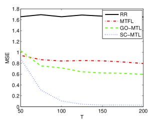
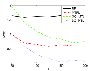
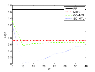
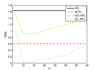
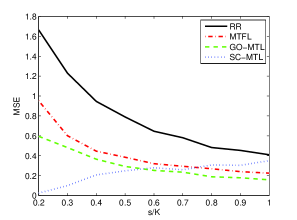
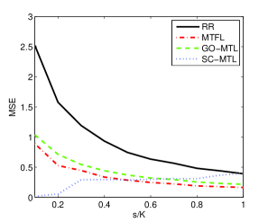
In the first experiment, we fix $K=10,d=20,s=2,\alpha=10,m=10,\sigma=0.1$ and study the statistical performance of the methods as a function of the number of tasks. The results, shown in Figure 1, clearly indicate that the proposed method outperforms the remaining approaches. In this experiment the number of atoms used by dictionary-based approaches, which here we denote by $K^{\prime}$ to avoid confusion with the number of atoms $K$ of the target dictionary, was equal to $K=10$. This gives an advantage to both GO-MTL and SC-MTL. We therefore also studied the performance of those methods in dependence on $K^{\prime}$. Figure 2, reporting this result, is in qualitative agreement with our theoretical analysis: the performance of SC-MTL is not too sensitive to $K^{\prime}$ if $K^{\prime}\geq K$, and the method still outperforms independent RR and MTFL if $K^{\prime}=4K$. On the other hand if $K^{\prime}<K$ the performance of the method quickly degrades. In the last experiment we study performance vs. the sparsity ratio $s/K$. Intuitively we would expect our method to have greater advantage over MTL if $s\ll K$. The results, shown in Figure 3, confirm this fact, also indicating that SC-MTL is outperformed by both GO-MTL and MTFL as sparsity becomes less pronounced ($s/K>0.6$).

4.3 Learning to learn optical character recognition

We have conducted experiments on real data to study the performance of our method in a learning to learn / transfer learning setting. To this end, we employed the NIST dataset, which is composed of a set of $14\times 14$ pixels images of handwritten characters (digits and lower and capital case letters, for a total of 52 characters).

We considered the following experimental protocol. First, a set of $20$ characters are chosen randomly as well as $n$ instances for each character. These are used to learn all possibilities of $1$-vs-$1$ train tasks, which makes $T=190$, each of which having $m=2n$ instances. The knowledge learned in this stage is employed to learn another set of target tasks. In our approach, the assumption that is made is that some of the components in the dictionary learned from the training tasks, can also be useful for representing the target tasks. In order to create the target tasks, another set of $10$ characters are chosen among the remaining set of characters in the dataset, inducing a set of $45$ $1$-vs-$1$ classification tasks. Since we are interested in the case where the training set size of the target tasks is small, we sample only $3$ instances for each character, hence $6$ examples per task.

In order to tune the hyperparameters of all compared approaches, we have also created another set of $45$ validation tasks by following the process previously described, simulating the target set of tasks. Note that there is not overlapping between the digits associated to the train, target and validation tasks.

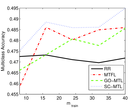
We have run $50$ trials of the above process for different values of $m$ and the average multiclass accuracy on the target tasks is reported in Figure 4.

Figure 4: Multiclassification accuracy of RR, MTFL GO-MTL and SC-MTL vs. the number of training instances in the transfer tasks, $m$.

4.4 Sparse coding of images with missing pixels

In the last experiment we consider a sparse coding problem (Olshausen & Field, 1996) of optical character images, with missing pixels. We employ the Binary Alphadigits dataset, which is composed of a set of binary $20\times 16$ images of all digits and capital letters (39 images for each character). In the following experiment only the digits are used. We regard each image as a task, hence the input space is the set of $320$ possible pixels indices, while the output space is the real interval $[0,1]$, representing the gray level. We sample $T=100,130,160,190,220,250$ images, equally divided among the $10$ possible digits. For each of these, a corresponding random set of $m=160$ pixel values are sampled (so the set of sample pixels varies from one image to another).

Figure 5: Transfer error vs. number of tasks T (Top) and vs. number of atoms K (Bottom) on the Binary Alphadigits dataset.

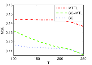
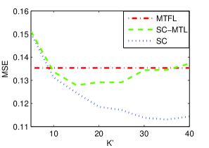
We test the performance of the dictionary learned by method (1) in a learning to learn setting, by choosing $100$ new images. The regularization parameter for each approach is tuned using cross validation. The results, shown in Figure 5, indicate some advantage of the proposed method over trace norm regularization. A similar trend, not reported here due to space constraints, is obtained in the multitask setting. Ridge regression performed significantly worse and is not shown in the figure. We also show as a reference the performance of sparse coding (SC) applied when all pixels are known.

With the aim of analyzing the atoms learned by the algorithm, we have carried out another experiment where we assume that there are $10$ underlying atoms (one for each digit). We compare the resultant dictionary to that obtained by sparse coding, where all pixels are known. The results are shown in Figure 6.

Figure 6: Dictionaries found by SC-MTL using $m=240$ pixels (missing $25\%$ pixels) per image (top) and by Sparse Coding employing all pixels (bottom).

5 Summary

In this paper, we have explored an application of sparse coding, which has been widely used in unsupervised learning and signal processing, to the domains of multitask learning and learning to learn. Our learning bounds provide a justification of this method and offer insights into its advantage over independent task learning and learning dense representation of the tasks. The bounds, which hold in a Hilbert space setting, depend on data dependent quantities which measure the intrinsic dimensionality of the data. Numerical simulations presented here indicate that sparse coding is a promising approach to multitask learning and can lead to significant improvements over competing methods.

In the future, it would be valuable to study extensions of our analysis to more general classes of code vectors. For example, we could use code sets $\mathcal{C}_{\alpha}$ which arise from structured sparsity norms, such as the group Lasso, see e.g. (Jenatton et al., 2011; Lounici et al., 2011) or other families of regularizers. A concrete example which comes to mind is to choose $K=Qr$, $Q,r\in{\mathbb{N}}$ and a partition ${\mathcal{J}}=\{\{(q-1)r+1,\dots,qr\}:q=1,\dots,Q\}$ of the index set $\{1,\dots,K\}$ into contiguous index sets of size $r$. Then using a norm of the type $\|\gamma\|=\|\gamma\|_{1}+\sum_{J\in\mathcal{J}}\|\gamma_{J}\|_{2}$ will encourage codes which are sparse and use only few of the groups in ${\mathcal{J}}$. Using the ball associated with this norm as our set of codes would allow to model sets of tasks which are divided into groups. A further natural extension of our method is nonlinear dictionary learning in which the dictionary columns correspond to functions in a reproducing kernel Hilbert space and the tasks are expressed as sparse linear combinations of such functions.

Appendix

In this appendix, we present the proof of Theorems 1 and 2. We begin by introducing some more notation and auxiliary results.

Appendix A Notation and tools

Issues of measurability will be ignored throughout, in particular, if $\tciFourier$ is a class of real valued functions on a domain $\mathcal{X}$ and $X$ a random variable with values in $\mathcal{X}$ then we will always write ${\mathbb{E}}\sup_{f\in\tciFourier}f\left(X\right)$ to mean $\sup\left\{{\mathbb{E}}\max_{f\in\tciFourier_{0}}f\left(X\right):\tciFourier_{0}\subseteq\tciFourier\text{, }\tciFourier_{0}\text{ finite}\right\}$.

In the sequel $H$ denotes a finite or infinite dimensional Hilbert space with inner product $\left\langle\cdot,\cdot\right\rangle$ and norm $\left\|\cdot\right\|$. If $T$ is a bounded linear operator on $H$ its operator norm is written $\left\|T\right\|_{\infty}=\sup\left\{\left\|Tx\right\|:\left\|x\right\|=1\right\}$.

Members of $H$ are denoted with lower case italics such as $x,v,w$, vectors composed of such vectors are in bold lower case, i.e. $\mathbf{x}=\left(x_{1},\ldots,x_{m}\right)$ or $\mathbf{v=}\left(v_{1},\ldots,v_{n}\right)$, where $m$ or $n$ are explained in the context.

Let $B$ be the unit ball in $H$. An example is a pair $z=\left(x,y\right)\in B\times\mathbb{R}=:\mathcal{Z}$, a sample is a vector of such pairs $\mathbf{z}=\left(z_{1},\ldots,z_{m}\right)=\left(\left(x_{1},y_{1}\right),\ldots,\left(x_{m},y_{m}\right)\right)$. Here we also write $\mathbf{z}=\left(\mathbf{x},\mathbf{y}\right)$, with $\mathbf{x}=\left(x_{1},\ldots,x_{m}\right)\in H^{m}$ and $\mathbf{y}=\left(y_{1},\ldots,y_{m}\right)\in\mathbb{R}^{m}$.

A multisample is a vector $\mathbf{Z}=\left(\mathbf{z}_{1},\ldots,\mathbf{z}_{T}\right)$ composed of samples. We also write $\mathbf{Z}=\left(\mathbf{X},\mathbf{Y}\right)$ with $\mathbf{X=}\left(\mathbf{x}_{1},\ldots,\mathbf{x}_{T}\right)$.

For members of $\mathbb{R}^{K}$ we use the greek letters $\gamma$ or $\beta$. Depending on context the inner product and euclidean norm on $\mathbb{R}^{K}$ will also be denoted with $\left\langle\cdot,\cdot\right\rangle$ and $\left\|.\right\|$. The $\ell_{1}$-norm $\left\|\cdot\right\|_{1}$ on $\mathbb{R}^{K}$ is defined by $\left\|\beta\right\|_{1}=\sum_{k=1}^{K}\left|\beta_{k}\right|$.

In the sequel we denote with $\mathcal{C}_{\alpha}$ the set $\left\{\beta\in\mathbb{R}^{K}:\left\|\beta\right\|_{1}\leq\alpha\right\}$, abbreviate $\mathcal{C}$ for the $\ell_{1}$-unit ball $\mathcal{C}_{1}$. The canonical basis of $\mathbb{R}^{K}$ is denoted $e_{1},\ldots,e_{K}$. Unless otherwise specified the summation over the index $i$ will always run from $1$ to $m$, $t$ will run from $1$ to $T$, and $k$ will run from $1$ to $K$.

A.1 Covariances

For $\mathbf{x\in}H^{m}$ the empirical covariance operator $\hat{\Sigma}\left(\mathbf{x}\right)$ is specified by

$$\left\langle\hat{\Sigma}\left(\mathbf{x}\right)v,w\right\rangle=\frac{1}{m}\sum_{i}\left\langle v,x_{i}\right\rangle\left\langle x_{i},w\right\rangle,\text{ }v,w\in H\text{.}$$

The definition implies the inequality

$$\sum_{i}\left\langle v,x_{i}\right\rangle^{2}=m\left\langle\hat{\Sigma}\left(\mathbf{x}\right)v,v\right\rangle\leq m\left\|\hat{\Sigma}\left(\mathbf{x}\right)\right\|_{\infty}\left\|v\right\|^{2}\text{.}$$ (6)

It also follows that ${\mathrm{t}r}\left(\hat{\Sigma}\left(\mathbf{x}\right)\right)=\left(1/m\right)\sum_{i}\left\|x_{i}\right\|^{2}$.

For a multisample $\mathbf{X}\in H^{mT}$ we will consider two quantities defined in terms of the empirical covariances.

$$S_{1}\left(\mathbf{X}\right) = \frac{1}{T}\sum_{t}\left\|\hat{\Sigma}\left(\mathbf{x}_{t}\right)\right\|_{1}:=\frac{1}{T}\sum_{t}{\mathrm{t}r}\left(\hat{\Sigma}\left(\mathbf{x}_{t}\right)\right)$$

$$S_{\infty}\left(\mathbf{X}\right) = \frac{1}{T}\sum_{t}\left\|\hat{\Sigma}\left(\mathbf{x}_{t}\right)\right\|_{\infty}:=\frac{1}{T}\sum_{t}\lambda_{\max}\left(\hat{\Sigma}\left(\mathbf{x}_{t}\right)\right)$$

where $\lambda_{\max}$ is the largest eigenvalue. If all data points $x_{ti}$ lie in the unit ball of $H$ then $S_{1}\left(\mathbf{X}\right)\leq 1$. Of course $S_{1}\left(\mathbf{X}\right)$ can also be written as the trace of the total covariance $\left(1/T\right)\sum_{t}\hat{\Sigma}\left(\mathbf{x}_{t}\right)$, while $S_{\infty}\left(\mathbf{X}\right)$ will always be at least as large as the largest eigenvalue of the total covariance. We always have $S_{\infty}\left(\mathbf{X}\right)\leq S_{1}\left(\mathbf{X}\right)$, with equality only if the data is one-dimensional for all tasks. The quotient $S_{1}\left(\mathbf{X}\right)/S_{\infty}\left(\mathbf{X}\right)$ can be regarded as a crude measure of the effective dimensionality of the data. If the data have a high dimensional distribution for each task then $S_{\infty}\left(\mathbf{X}\right)$ can be considerably smaller than $S_{1}\left(\mathbf{X}\right)$.

A.2 Concentration inequalities

Let $\mathcal{X}$ be any space. For $\mathbf{x}\in\mathcal{X}^{n}$, $1\leq k\leq n$ and $y\in\mathcal{X}$ we use $\mathbf{x}_{k\leftarrow y}$ to denote the object obtained from $\mathbf{x}$ by replacing the $k$-th coordinate of $\mathbf{x}$ with $y$. That is

$$\mathbf{x}_{k\leftarrow y}=\left(x_{1},\dots,x_{k-1},y,x_{k+1},\dots,x_{n}\right)\text{.}$$

The concentration inequality in part (i) of the following theorem, known as the bounded difference inequality is given in (McDiarmid, 1998). A proof of inequality (ii) is given in (Maurer, 2006).

Theorem 3.

Let $F:\mathcal{X}^{n}\rightarrow\mathbb{R}$ and define $A$ and $B$ by

$$A^{2} = \sup_{\mathbf{x}\in\mathcal{X}^{n}}\sum_{k=1}^{n}\sup_{y_{1},y_{2}\in\mathcal{X}}\left(F\left(\mathbf{x}_{k\leftarrow y_{1}}\right)-F\left(\mathbf{x}_{k\leftarrow y_{2}}\right)\right)^{2}$$

$$B^{2} = \sup_{\mathbf{x}\in\mathcal{X}^{n}}\sum_{k=1}^{n}\left(F\left(\mathbf{x}\right)-\inf_{y\in\mathcal{X}}F\left(\mathbf{x}_{k\leftarrow y}\right)\right)^{2}.$$

Let $\mathbf{X}=\left(X_{1},\dots,X_{n}\right)$ be a vector of independent random variables with values in $\mathcal{X}$, and let $\mathbf{X}^{\prime}$ be i.i.d. to $\mathbf{X}$. Then for any $s>0$

(i) $\Pr\left\{F\left(\mathbf{X}\right)>{{\mathbb{E}}}F\left(\mathbf{X}^{\prime}\right)+s\right\}\leq e^{-2s^{2}/A^{2}};$

(ii) $\Pr\left\{F\left(\mathbf{X}\right)>{{\mathbb{E}}}F\left(\mathbf{X}^{\prime}\right)+s\right\}\leq e^{-s^{2}/\left(2B^{2}\right)}.$

A.3 Rademacher and Gaussian averages

We will use the term Rademacher variables for any set of independent random variables, uniformly distributed on $\left\{-1,1\right\}$, and reserve the symbol $\sigma$ for Rademacher variables. A set of random variables is called orthogaussian if the members are independent ${\mathcal{N}}\left(0,1\right)$-distributed (standard normal) variables and reserve the letter $\zeta$ for standard normal variables. Thus $\sigma_{1},\sigma_{2},\ldots,\sigma_{i},\ldots,\sigma_{11},\ldots,\sigma_{ij}$ etc. will always be independent Rademacher variables and $\zeta_{1},\zeta_{2},\ldots,\zeta_{i},\ldots,\zeta_{11},\ldots,\zeta_{ij}$ will always be orthogaussian.

For $A\subseteq\mathbb{R}^{n}$ we define the Rademacher and Gaussian averages of $A$ (Ledoux & Talagrand, 1991; Bartlett & Mendelson, 2002) as

$$\mathcal{R}\left(A\right) = \mathbb{E}_{\sigma}\sup_{\left(x_{1},\ldots,x_{n}\right)\in A}\frac{2}{n}\sum_{i=1}^{n}\sigma_{i}x_{i}\text{, }$$

$$\mathcal{G}\left(A\right) = \mathbb{E}_{\zeta}\sup_{\left(x_{1},\ldots,x_{n}\right)\in A}\frac{2}{n}\sum_{i=1}^{n}\zeta_{i}x_{i}.$$

If $\mathcal{F}$ is a class of real valued functions on a space $\mathcal{X}$ and $\mathbf{x}=\left(x_{1},\ldots,x_{n}\right)\in\mathcal{X}^{n}$ we write

$$\mathcal{F}\left(\mathbf{x}\right)=\mathcal{F}\left(x_{1},\ldots,x_{n}\right)$$

$$=\left\{\left(f\left(x_{1}\right),\ldots,f\left(x_{n}\right)\right):f\in\mathcal{F}\right\}\subseteq\mathbb{R}^{n}.$$

The empirical Rademacher and Gaussian complexities of $\mathcal{F}$ on $\mathbf{x}$ are respectively $\mathcal{R}\left(\mathcal{F}\left(\mathbf{x}\right)\right)$ and $\mathcal{G}\left(\mathcal{F}\left(\mathbf{x}\right)\right)$.

The utility of these concepts for learning theory comes from the following key-result (see (Bartlett & Mendelson, 2002; Koltchinskii & Panchenko, 2002)), stated here in two portions for convenience in the sequel.

Theorem 4.

Let $\mathcal{F}$ be a real-valued function class on a space $\mathcal{X}$ and $\mu_{1},\ldots,\mu_{m}$ be probability measures on $\mathcal{X}$ with product measure $\mathbf{\mu}=\prod_{i}\mu_{i}$ on $\mathcal{X}^{m}$. For $\mathbf{x}\in\mathcal{X}^{m}$ define

$$\Phi\left(\mathbf{x}\right)=\sup_{f\in\mathcal{F}}\frac{1}{m}\sum_{i=1}^{m}\left(\mathbb{E}_{x\sim\mu_{i}}\left[f\left(x\right)\right]-f\left(x_{i}\right)\right).$$

Then $\mathbb{E}_{\mathbf{x}\sim\mathbf{\mu}}\left[\Phi\left(\mathbf{x}\right)\right]\leq\mathbb{E}_{\mathbf{x}\sim\mathbf{\mu}}\mathcal{R}\left(\mathcal{F}\left(\mathbf{x}\right)\right)$.

Proof.

For any realization $\sigma=\sigma_{1},\ldots,\sigma_{m}$ of the Rademacher variables

$$\mathbb{E}_{\mathbf{x}\sim\mathbf{\mu}}\left[\Phi\left(\mathbf{x}\right)\right]$$

$$=\mathbb{E}_{\mathbf{x}\sim\mathbf{\mu}}\sup_{f\in\mathcal{F}}\frac{1}{m}\mathbb{E}_{\mathbf{x}^{\prime}\sim\mathbf{\mu}}\sum_{i=1}^{m}\left(f\left(x_{i}^{\prime}\right)-f\left(x_{i}\right)\right)$$

$$\leq\mathbb{E}_{\mathbf{x,x}^{\prime}\sim\mathbf{\mu}\times\mathbf{\mu}}\sup_{f\in\mathcal{F}}\frac{1}{m}\sum_{i=1}^{m}\sigma_{i}\left(f\left(x_{i}^{\prime}\right)-f\left(x_{i}\right)\right),$$

because of the symmetry of the measure $\mathbf{\mu}\times\mathbf{\mu}\left(\mathbf{x},\mathbf{x}^{\prime}\right)\mathbf{=}\prod_{i}\mu_{i}\times\prod_{i}\mu_{i}\left(\mathbf{x},\mathbf{x}^{\prime}\right)$under the interchange $x_{i}\leftrightarrow x_{i}^{\prime}$. Taking the expectation  in $\sigma$ and applying the triangle inequality gives the result.    

Theorem 5.

Let $\mathcal{F}$ be a $\left[0,1\right]$-valued function class on a space $\mathcal{X}$, and $\mathbf{\mu}$ as above. For $\delta>0$ we have with probability greater than $1-\delta$ in the sample $\mathbf{x}\sim\mathbf{\mu}$ that for all $f\in\mathcal{F}$

$$\mathbb{E}_{x\sim\mathbf{\mu}}\left[f\left(x\right)\right]\leq\frac{1}{m}\sum_{i=1}^{m}f\left(x_{i}\right)+\mathbb{E}_{\mathbf{x}\sim\mathbf{\mu}}\mathcal{R}\left(\mathcal{F}\left(\mathbf{x}\right)\right)+\sqrt{\frac{\ln\left(1/\delta\right)}{2m}}.$$

To prove this we apply the bounded-difference inequality ( part (i) of Theorem 3) to the function $\Phi$ of the previous theorem (see e.g. (Bartlett & Mendelson, 2002)). Under the conditions of this result, changing one of the $x_{i}$ will not change $\mathcal{R}\left(\mathcal{F}\left(\mathbf{x}\right)\right)$ by more than $2$, so again by the bounded difference inequality applied to $\mathcal{R}\left(\mathcal{F}\left(\mathbf{x}\right)\right)$ and a union bound we obtain the data dependent version

Corollary 6.

Let $\mathcal{F}$ and $\mathbf{\mu}$ be as above. For $\delta>0$ we have with probability greater than $1-\delta$ in the sample $\mathbf{x}\sim\mathbf{\mu}$ that for all $f\in\mathcal{F}$

$$\mathbb{E}_{x\sim\mathbf{\mu}}\left[f\left(x\right)\right]\leq\frac{1}{m}\sum_{i=1}^{m}f\left(x_{i}\right)+\mathcal{R}\left(\mathcal{F}\left(\mathbf{x}\right)\right)+\sqrt{\frac{9\ln\left(2/\delta\right)}{2m}}.$$

To bound Rademacher averages the following result is very useful (Bartlett & Mendelson, 2002; Ando & Zhang, 2005; Ledoux & Talagrand, 1991)

Lemma 7.

Let $A\subseteq\mathbb{R}^{n}$, and let $\psi_{1},\ldots,\psi_{n}$ be real functions such that $\psi_{i}\left(s\right)-\psi_{i}\left(t\right)\leq L\left|s-t\right|$,$\forall i$, and $s,t\in\mathbb{R}$. Define $\mathbf{\psi}\left(A\right)=\left\{\psi_{1}\left(x_{1}\right),\ldots,\psi_{n}\left(x_{n}\right):\left(x_{1},\ldots,x_{n}\right)\in A\right\}$. Then

$$\mathcal{R}\left(\mathbf{\psi}\left(A\right)\right)\leq L\mathcal{R}\left(A\right)\text{.}$$

Sometimes it is more convenient to work with gaussian averages which can be used instead, by virtue of the next lemma. For a proof see e.g. (Ledoux & Talagrand, 1991)

Lemma 8.

For $A\subseteq\mathbb{R}^{k}$ we have $\mathcal{R}\left(A\right)\leq\sqrt{\pi/2}~{}\mathcal{G}\left(A\right)$.

The next result is known as Slepian’s lemma ((Slepian, 1962), (Ledoux & Talagrand, 1991)).

Theorem 9.

Let $\Omega$ and $\Xi$ be mean zero, separable Gaussian processes indexed by a common set $\mathcal{S}$, such that

$$\mathbb{E}\left(\Omega_{s_{1}}-\Omega_{s_{2}}\right)^{2}\leq\mathbb{E}\left(\Xi_{s_{1}}-\Xi_{s_{2}}\right)^{2}\text{ for all }s_{1},s_{2}\in\mathcal{S}\text{.}$$

Then

$$\mathbb{E}\sup_{s\in\mathcal{S}}\Omega_{s}\leq\mathbb{E}\sup_{s\in\mathcal{S}}\Xi_{s}.$$

Appendix B Proofs

B.1 Multitask learning

In this section we prove Theorem 1. It is an immediate consequence of Hoeffding’s inequality and the following uniform bound on the estimation error.

Theorem 10.

Let $\delta>0$, fix $K$ and let $\mu_{1},\ldots,\mu_{T}$ be probability measures on $H\times\mathbb{R}$. With probability at least $1-\delta$ in the draw of $\mathbf{Z}\sim\prod_{t=1}^{T}\mu_{t}$ we have for all $D\in\mathcal{D}_{K}$ and all $\mathbf{\gamma}\in\mathcal{C}_{\alpha}^{T}\mathcal{\ }$that

$$\frac{1}{T}\sum_{t=1}^{T}{\mathbb{E}}_{\left(x,y\right)\sim\mu_{t}}\left[\ell\left(\left\langle D\gamma_{t},x\right\rangle,y\right)\right]\\ -\frac{1}{mT}\sum_{t=1}^{T}\sum_{i=1}^{m}\ell\left(\left\langle D\gamma_{t},x_{ti}\right\rangle,y_{ti}\right)\\ \leq L\alpha\sqrt{\frac{2S_{1}\left(\mathbf{X}\right)\left(K+12\right)}{mT}}\\ +L\alpha\sqrt{\frac{8S_{\infty}\left(\mathbf{X}\right)\ln\left(2K\right)}{m}}+\sqrt{\frac{9\ln 2/\delta}{2mT}}.$$

The proof of this theorem requires auxiliary results. Fix $\mathbf{X}\in H^{mT}$ and for $\mathbf{\gamma}=\left(\gamma_{1},\ldots,\gamma_{T}\right)\in\left(\mathbb{R}^{K}\right)^{T}$ define the random variable

$$F_{\mathbf{\gamma}}=F_{\mathbf{\gamma}}\left(\mathbf{\sigma}\right)=\sup_{D\in\mathcal{D}_{K}}\sum_{t,i}\sigma_{ti}\left\langle D\gamma_{t},x_{ti}\right\rangle.$$ (7)

Lemma 11.

(i) If $\mathbf{\gamma}=(\gamma_{1},\dots,\gamma_{T})$ satisfies $\left\|\gamma_{t}\right\|\leq 1$ for all $t$, then

$${\mathbb{E}}F_{\mathbf{\gamma}}\leq\sqrt{mTK~{}S_{1}\left(\mathbf{X}\right)}.$$

(ii) If $\mathbf{\gamma}$ satisfies $\left\|\gamma_{t}\right\|_{1}\leq 1$ for all $t$, then for any $s\geq 0$

$$\Pr\left\{F_{\mathbf{\gamma}}\geq{\mathbb{E}}\left[F_{\mathbf{\gamma}}\right]+s\right\}\leq\exp\left(\frac{-s^{2}}{8mT~{}S_{\infty}\left(\mathbf{X}\right)}\right).$$

Proof.

(i) We observe that

${\mathbb{E}}F_{\mathbf{\gamma}}=\mathbb{E}\,\underset{D}{{\mathrm{s}up}}\underset{k}{\sum}\left\langle De_{k},\underset{t,i}{\sum}\sigma_{ti}\gamma_{tk}x_{ti}\right\rangle\\$

$$\leq \sup_{D}\left(\sum_{k}\left\|De_{k}\right\|^{2}\right)^{1/2}{\mathbb{E}}\left(\sum_{k}\left\|\sum_{t,i}\sigma_{ti}\gamma_{tk}x_{ti}\right\|^{2}\right)^{1/2}$$

$$\leq \sqrt{K}\left(\underset{k}{\sum}\mathbb{E}\left\|\underset{t,i}{\sum}\sigma_{ti}\gamma_{tk}x_{ti}\right\|^{2}\right)^{1/2}$$

$$= \sqrt{K}\left(\underset{k,t,i}{\sum}\left|\gamma_{tk}\right|^{2}\left\|x_{ti}\right\|^{2}\right)^{1/2}$$

$$= \sqrt{K}\left(\underset{t}{\sum}\left(\underset{k}{\sum}\left|\gamma_{tk}\right|^{2}\right)\underset{i}{\sum}\left\|x_{ti}\right\|^{2}\right)^{1/2}$$

$$\leq \sqrt{K\sum_{t,i}\left\|x_{ti}\right\|^{2}}=\sqrt{mTK~{}S_{1}\left(\mathbf{X}\right)}.$$

(ii) For any configuration $\mathbf{\sigma}$ of the Rademacher variables let $D\left(\mathbf{\sigma}\right)$ be the maximizer in the definition of $F_{\mathbf{\gamma}}\left(\mathbf{\sigma}\right)$. Then for any $s\in\left\{1,\ldots,T\right\}$, $j\in\left\{1,\ldots,m\right\}$ and any $\sigma^{\prime}\in\left\{-1,1\right\}$ to replace $\sigma_{sj}$ we have

$$F_{\mathbf{\gamma}}\left(\mathbf{\sigma}\right)-F_{\mathbf{\gamma}}\left(\mathbf{\sigma}_{\left(sj\right)\leftarrow\sigma^{\prime}}\right)\leq 2\left|\left\langle D\left(\mathbf{\sigma}\right)\gamma_{s},x_{sj}\right\rangle\right|.$$

Using the inequality (6) we then obtain

$\sum_{sj}\left(F_{\gamma}\left(\mathbf{\sigma}\right)-\inf_{\sigma^{\prime}\in\left\{-1,1\right\}}F_{\mathbf{\gamma}}\left(\mathbf{\sigma}_{\left(sj\right)\leftarrow\sigma^{\prime}}\right)\right)^{2}$

$$\leq 4\sum_{t,i}\left\langle D\left(\mathbf{\sigma}\right)\gamma_{t},x_{ti}\right\rangle^{2}$$

$$\leq 4m\sum_{t}\left\|\hat{\Sigma}\left(\mathbf{x}_{t}\right)\right\|_{\infty}\left\|D\left(\mathbf{\sigma}\right)\gamma_{t}\right\|^{2}$$

$$\leq 4m\sum_{t}\left\|\hat{\Sigma}\left(\mathbf{x}_{t}\right)\right\|_{\infty}.$$

In the last inequality we used the fact that for any $D\in\mathcal{D}_{K}$ we have $\left\|D\gamma_{t}\right\|\leq\sum_{k}\left|\gamma_{tk}\right|\left\|De_{k}\right\|\leq\left\|\gamma_{t}\right\|_{1}\leq 1$. The conclusion now follows from part (ii) of Theorem 3.    

Proposition 12.

For every fixed $\mathbf{Z}=\left(\mathbf{X,Y}\right)\in\left(H\times\mathbb{R}\right)^{mT}$ we have

${\mathbb{E}}_{\sigma}\sup_{D\in D,\mathbf{\gamma}\in\left(\mathcal{C}_{\alpha}\right)^{T}}\sum_{t,i}\sigma_{it}\ell\left(\left\langle D\gamma_{t},x_{ti}\right\rangle,y_{ti}\right)$

$$\leq L\alpha\sqrt{2mTS_{1}\left(\mathbf{X}\right)\left(K+12\right)}+L\alpha T\sqrt{8mS_{\infty}\left(\mathbf{X}\right)\ln\left(2K\right)}.$$

Proof.

It suffices to prove the result for $\alpha=1$, the general result being a consequence of rescaling. By Lemma 7 and the Lipschitz properties of the loss function $\ell$ we have

${\mathbb{E}}_{\sigma}\sup_{D\in{\mathcal{D}}_{K},\mathbf{\gamma}\in\left(\mathcal{C}\right)^{T},}\sum_{t,i}\sigma_{it}\ell\left(\left\langle D\gamma_{t},x_{ti}\right\rangle,y_{ti}\right)$

$$\leq L{\mathbb{E}}_{\sigma}\sup_{D\in{\mathcal{D}}_{K},\mathbf{\gamma}\in\left(\mathcal{C}\right)^{T},}\sum_{t,i}\sigma_{it}\left\langle D\gamma_{t},x_{ti}\right\rangle.$$ (8)

Since linear functions on a compact convex set attain their maxima at the extreme points, we have

$${\mathbb{E}}\sup_{D\in{\mathcal{D}}_{K},\mathbf{\gamma}\in(\mathcal{C})^{T},}\sum_{t=1}^{T}\sum_{i=1}^{m}\sigma_{it}\left\langle D\gamma_{t},x_{ti}\right\rangle={\mathbb{E}}\max_{\mathbf{\gamma}\in\text{ext}\left(\mathcal{C}\right)^{T}}F_{\mathbf{\gamma}},$$ (9)

where $F_{\mathbf{\gamma}}$ is defined as in (7). Let $c=\sqrt{mKTS_{1}\left(\mathbf{X}\right)}$. Now for any $\delta\geq 0$ we have, since $F_{\mathbf{\gamma}}\geq 0$,

${\mathbb{E}}\max_{\mathbf{\gamma}\in\text{ext}\left(\mathcal{C}\right)^{T}}F_{\mathbf{\gamma}}=\int_{0}^{\infty}\Pr\left\{\max_{\mathbf{\gamma}\in\text{ext}\left(\mathcal{C}\right)^{T}}F_{\mathbf{\gamma}}>s\right\}ds\\$

$$\leq c+\delta+\sum_{\mathbf{\gamma}\in\left(\text{ext}\left(\mathcal{C}\right)\right)^{T}}\int_{\sqrt{mKTS_{1}\left(\mathbf{X}\right)}+\delta}^{\infty}\Pr\left\{F_{\mathbf{\gamma}}>s\right\}ds$$

$$\leq c+\delta+\sum_{\mathbf{\gamma}\in\left(\text{ext}\left(\mathcal{C}\right)\right)^{T}}\int_{\delta}^{\infty}\Pr\left\{F_{\mathbf{\gamma}}>{\mathbb{E}}F_{\mathbf{\gamma}}+s\right\}ds$$

$$\leq c+\delta+\left(2K\right)^{T}\int_{\delta}^{\infty}\exp\left(\frac{-s^{2}}{8mTS_{\infty}\left(\mathbf{X}\right)}\right)ds$$

$$\leq c+\delta+\frac{4mTS_{\infty}\left(\mathbf{X}\right)\left(2K\right)^{T}}{\delta}\exp\left(\frac{-\delta^{2}}{8mTS_{\infty}\left(\mathbf{X}\right)}\right).$$

Here the first inequality follows from the fact that probabilities never exceed 1 and a union bound. The second inequality follows from Lemma 11, part (i), since ${\mathbb{E}}F_{\mathbf{k}}\leq\sqrt{mKTS_{1}\left(\mathbf{X}\right)}$. The third inequality follows from Lemma 11, part (ii), and the fact that the cardinality of ext$\left(\mathcal{C}\right)$ is $2K$, and the last inequality follows from a well known estimate on Gaussian random variables. Setting $\delta=\sqrt{8mTS_{\infty}\left(\mathbf{X}\right)\ln\left(e\left(2K\right)^{T}\right)}$ we obtain with some easy simplifying estimates

${\mathbb{E}}\max_{\mathbf{\gamma}\in\text{ext}\left(\mathcal{C}\right)^{T}}F_{\mathbf{\gamma}}\leq\sqrt{2mT\left(K+12\right)S_{1}\left(\mathbf{X}\right)}$

$$+T\sqrt{8mS_{\infty}\left(\mathbf{X}\right)\ln\left(2K\right)},$$

which together with (8) and (9) gives the result.    

Theorem 10 now follows from Corollary 6.

If the set $\mathcal{C}_{\alpha}$ is replaced by any other subset $\mathcal{C}^{\prime}$ of the $\ell_{2}$-ball of radius $\alpha$, a similar proof strategy can be employed. The denominator in the exponent of Lemma 11-(ii) then obtains another factor of $\sqrt{K}$. The union bound over the extreme points in ext$\left(\mathcal{C}\right)$ in the previous proposition can be replaced by a union bound over a cover $\mathcal{C}^{\prime}$. This leads to the alternative result mentioned in Remark 5 following the statement of Theorem 1.

Another modification leads to a bound for the method presented in (Kumar & Daumé III, 2012), where the constraint $\left\|De_{k}\right\|\leq 1$ is replaced by $\left\|D\right\|_{2}\leq\sqrt{K}$ (here $\left\|\cdot\right\|_{2}$ is the Frobenius or Hilbert Schmidt norm) and the constraint $\left\|\gamma_{t}\right\|_{1}\leq\alpha,\forall t$ is replaced by $\sum\left\|\gamma_{t}\right\|_{1}\leq\alpha T$. To explain the modification we set $\alpha=1$. Part (i) of Lemma 11 is easily verified. The union bound over $\left(\text{ext}\left(\mathcal{C}\right)\right)^{T}$ in the previous proposition is replaced by a union bound over the $2TK$ extreme points of the $\ell_{1}$-Ball of radius $T$ in $\mathbb{R}^{TK}$. For part (ii) we use the fact that the concentration result is only needed for $\mathbf{\gamma}$ being an extreme point (so that it involves only a single task) and obtain the bound $\sum_{t}\left\|\hat{\Sigma}\left(\mathbf{x}_{t}\right)\right\|_{\infty}\left\|D\gamma_{t}\right\|^{2}\leq TKS_{\infty}^{\prime}\left(\mathbf{X}\right)$, leading to

$$\Pr\left\{F_{\mathbf{\gamma}}\geq E\left[F_{\mathbf{\gamma}}\right]+s\right\}\leq\exp\left(\frac{-s^{2}}{8mTK~{}S_{\infty}^{\prime}\left(\mathbf{X}\right)}\right).$$

Proceeding as above we obtain the excess risk bound

$L\alpha\sqrt{\frac{2S_{1}\left(\mathbf{X}\right)\left(K+12\right)}{mT}}+L\alpha\sqrt{\frac{8KS_{\infty}^{\prime}\left(\mathbf{X}\right)\ln\left(2KT\right)}{m}}$

$$+\sqrt{\frac{8\ln 4/\delta}{mT}},$$

to replace the bound in Theorem 1. The factor $\sqrt{K}$ in the second term seems quite weak, but it must be borne in mind that the constraint $\left\|D\right\|_{2}\leq\sqrt{K}$ is much weaker than $\left\|De_{k}\right\|\leq 1$, and allows for a smaller approximation error. If we retain $\left\|De_{k}\right\|\leq 1$ and only modify the $\gamma$-constraint to $\sum\left\|\gamma_{t}\right\|_{1}\leq\alpha T$ the $\sqrt{K}$ in the second term disappears and by comparison to Theorem 1 there is only and additional $\ln T$ and the switch from $S_{\infty}\left(\mathbf{X}\right)$ to $S_{\infty}^{\prime}\left(\mathbf{X}\right)$, reflecting the fact that $\sum\left\|\gamma_{t}\right\|_{1}\leq\alpha T$ is a much weaker constraint than $\left\|\gamma_{t}\right\|_{1}\leq\alpha,\forall t$, so that, again, a smaller minimum in (1) is possible for the modified method.

B.2 Learning to learn

In this section we prove Theorem 2. The basic strategy is as follows. Recall the definition (4) of the measure $\rho_{\mathcal{E}}$, which governs the generation of a training sample in the environment $\mathcal{E}$. On a given training sample $\mathbf{z\sim}\rho_{\mathcal{E}}$ the algorithm $A_{D}$ as defined in (3) incurs the empirical risk

$$\hat{R}_{D}\left(\mathbf{z}\right)=\min_{\gamma\in\mathcal{C}_{\alpha}}\frac{1}{m}\sum_{i=1}^{m}\ell\left(\left\langle D\gamma,x_{i}\right\rangle,y_{i}\right).$$

The algorithm $A_{D}$, essentially being the Lasso, has very good estimation properties, so $\hat{R}_{D}\left(\mathbf{z}\right)$ will be close to the true risk of $A_{D}$ in the corresponding task. This means that we only really need to estimate the expected empirical risk ${\mathbb{E}}_{\mathbf{z\sim}\rho_{\mathcal{E}}}\hat{R}_{D}\left(\mathbf{z}\right)$ of $A_{D}$ on future tasks. On the other hand the minimization problem (1) can be written as

$$\min_{D\in\mathcal{D}_{K}}\frac{1}{T}\sum_{t=1}^{T}\hat{R}_{D}\left(\mathbf{z}_{t}\right)\text{ with }\mathbf{Z=}\left(z_{1},\ldots,z_{T}\right)\sim\left(\rho_{\mathcal{E}}\right)^{T},$$

with dictionary $D\left(\mathbf{Z}\right)$ being the minimizer. If $\mathcal{D}_{K}$ is not too large this should be similar to ${\mathbb{E}}_{\mathbf{z\sim}\rho_{\mathcal{E}}}\hat{R}_{D\left(\mathbf{Z}\right)}\left(\mathbf{z}\right)$. In the sequel we make this precise.

Lemma 13.

For $v\in H$ with $\left\|v\right\|\leq 1$ and $\mathbf{x}\in H^{m}$ let $F$ be the random variable

$$F=\left|\left\langle v,\sum_{i}\sigma_{i}x_{i}\right\rangle\right|\text{.}$$

Then (i) ${\mathbb{E}}F\leq\sqrt{m}\left\|\hat{\Sigma}\left(\mathbf{x}\right)\right\|_{\infty}^{1/2}$ and (ii) for $t\geq 0$

$$\Pr\left\{F>{\mathbb{E}}F+s\right\}\leq\exp\left(\frac{-s^{2}}{2m\left\|\hat{\Sigma}\left(\mathbf{x}\right)\right\|_{\infty}}\right).$$

Proof.

(i). Using Jensen’s inequality and (6) we get

$${\mathbb{E}}F \leq \left({\mathbb{E}}\left\langle v,\sum_{i}\sigma_{i}x_{i}\right\rangle^{2}\right)^{1/2}$$

$$= \left(\sum_{i}\left\langle v,x_{i}\right\rangle^{2}\right)^{1/2}\leq\sqrt{m\left\|\hat{\Sigma}\left(\mathbf{x}\right)\right\|_{\infty}}.$$

(ii) Let $\mathbf{\sigma}$ be any configuration of the Rademacher variables. For any $\sigma^{\prime},\sigma^{\prime\prime}\in\left\{-1,1\right\}$ to replace $\sigma_{sj}$ we have

$$F\left(\mathbf{\sigma}_{\left(sj\right)\leftarrow\sigma^{\prime}}\right)-F\left(\mathbf{\sigma}_{\left(sj\right)\leftarrow\sigma^{\prime\prime}}\right)\leq 2\left|\left\langle v,x_{j}\right\rangle\right|,$$

so the conclusion follows from the bounded difference inequality, Theorem 3 (i).    

Lemma 14.

For $v_{1},\ldots,v_{K}\in H$ satisfying $\left\|v_{k}\right\|\leq 1$, $\mathbf{x}\in H^{m}$ we have

$${\mathbb{E}}\max_{k}\left|\left\langle v_{k},\sum_{i}\sigma_{i}x_{i}\right\rangle\right|\leq\sqrt{2m\left\|\hat{\Sigma}\left(\mathbf{x}\right)\right\|_{\infty}}\left(2+\sqrt{\ln K}\right).$$

Proof.

Let $F_{k}=\left|\left\langle v_{k},\sum_{i}\sigma_{i}x_{i}\right\rangle\right|$. Setting $c=\sqrt{m\left\|\hat{\Sigma}\left(\mathbf{x}\right)\right\|_{\infty}}$ and using integration by parts we have for $\delta\geq 0$

${\mathbb{E}}\max_{k}F_{k}$

$$\leq c+\delta+\int_{\sqrt{m\left\|\hat{\Sigma}\left(\mathbf{x}\right)\right\|_{\infty}}+\delta}^{\infty}\max_{k}\Pr\left\{F_{k}\geq s\right\}ds$$

$$\leq c+\delta+\sum_{k}\int_{\delta}^{\infty}\Pr\left\{F_{k}\geq{\mathbb{E}}F_{k}+s\right\}ds$$

$$\leq c+\delta+\sum_{k}\int_{\delta}^{\infty}\exp\left(\frac{-s^{2}}{2m\left\|\hat{\Sigma}\left(\mathbf{x}\right)\right\|_{\infty}}\right)ds$$

$$\leq c+\delta+\frac{mK\left\|\hat{\Sigma}\left(\mathbf{x}\right)\right\|_{\infty}}{\delta}\exp\left(\frac{-\delta^{2}}{2m\left\|\hat{\Sigma}\left(\mathbf{x}\right)\right\|_{\infty}}\right).$$

Above the first inequality is trivial, the second follows from Lemma 13 (i) and a union bound, the third inequality follows from Lemma 13 (ii) and the last from a well known approximation. The conclusion follows from substitution of $\delta=\sqrt{2m\left\|\hat{\Sigma}\left(\mathbf{x}\right)\right\|_{\infty}\ln\left(eK\right)}$.    

Proposition 15.

Let $S_{\infty}\left(\mathcal{E}\right):={\mathbb{E}}_{\tau\sim\mathcal{E}}{\mathbb{E}}_{\left(\mathbf{x,y}\right)\sim\mu_{\tau}^{m}}\left\|\hat{\Sigma}\left(\mathbf{x}\right)\right\|_{\infty}$. With probability at least $1-\delta$ in the multisample $\mathbf{Z}\sim\rho_{\mathcal{E}}^{T}$

$$\sup_{D\in\mathcal{D}_{K}}R_{\mathcal{E}}\left(A_{D}\right)-\frac{1}{T}\sum_{t=1}^{T}\hat{R}_{D}\left(\mathbf{z}_{t}\right)$$

$$\leq L\alpha K\sqrt{\frac{2\pi S_{1}\left(\mathbf{X}\right)}{T}}$$

$$+ 4L\alpha\sqrt{\frac{S_{\infty}\left(\mathcal{E}\right)\left(2+\ln K\right)}{m}}+\sqrt{\frac{9\ln 2/\delta}{2T}}.$$

Proof.

Following our strategy we write (abbreviating $\rho=\rho_{\mathcal{E}}$)

$$\sup_{D\in\mathcal{D}_{K}}R_{\mathcal{E}}\left(A_{D}\right)-\frac{1}{T}\sum_{t=1}^{T}\hat{R}_{D}\left(\mathbf{z}_{t}\right)$$

$$\leq \sup_{D\in\mathcal{D}_{K}}{\mathbb{E}}_{\tau\sim\mathcal{E}}{\mathbb{E}}_{\mathbf{z}\sim\mu_{\tau}^{m}}$$

$$\left[{\mathbb{E}}_{\left(x,y\right)\sim\mu_{\tau}}\left[\ell\left(\left\langle A_{D}\left(\mathbf{z}\right),x\right\rangle,y\right)\right]-\hat{R}_{D}\left(\mathbf{z}\right)\right]$$

$$+ \sup_{D\in\mathcal{D}_{K}}{\mathbb{E}}_{\mathbf{z}\sim\rho}\left[\hat{R}_{D}\left(\mathbf{z}\right)\right]-\frac{1}{T}\sum_{t=1}^{T}\hat{R}_{D}\left(\mathbf{z}_{t}\right)$$

and proceed by bounding each of the two terms in turn.

For any fixed dictionary $D$ and any measure $\mu$ on $\mathcal{Z}$ we have

$${\mathbb{E}}_{\mathbf{z}\sim\mu^{m}}\left[{\mathbb{E}}_{\left(x,y\right)\sim\mu}\left[\ell\left(\left\langle A_{D}\left(\mathbf{z}\right),x\right\rangle,y\right)\right]-\hat{R}_{D}\left(\mathbf{z}\right)\right]$$

$$\leq {\mathbb{E}}_{\mathbf{z}\sim\mu^{m}}\sup_{\gamma\in\mathcal{C}_{\alpha}}\bigg{[}{\mathbb{E}}_{\left(x,y\right)\sim\mu}\left[\ell\left(\left\langle D\gamma,x\right\rangle,y\right)\right]$$

$$-\frac{1}{m}\sum_{i=1}^{m}\ell\left(\left\langle D\gamma,x_{i}\right\rangle,y_{i}\right)\bigg{]}$$

$$\leq \frac{2}{m}{\mathbb{E}}_{\mathbf{z}\sim\mu^{m}}{\mathbb{E}}_{\sigma}\sup_{\gamma\in\mathcal{C}_{\alpha}}\sum_{i=1}^{m}\sigma_{i}\ell\left(\left\langle D\gamma,x_{i}\right\rangle,y_{i}\right)\text{\small~{}~{} [Theorem \ref{Theorem Rademacher bound Expectation version}]}$$

$$\leq \frac{2L}{m}{\mathbb{E}}_{\mathbf{z}\sim\mu^{m}}{\mathbb{E}}_{\sigma}\sup_{\gamma\in\mathcal{C}_{\alpha}}\sum_{k}\gamma_{k}\left\langle De_{k},\sum_{i=1}^{m}\sigma_{i}x_{i}\right\rangle\text{\small~{}~{}[Lemma \ref{Lemma Rademacher Lipschitz}]}$$

$$\leq \frac{2L\alpha}{m}{\mathbb{E}}_{\mathbf{z}\sim\mu^{m}}{\mathbb{E}}_{\sigma}\max_{k}\left|\left\langle De_{k},\sum_{i=1}^{m}\sigma_{i}x_{i}\right\rangle\right|\text{\small~{}~{} [H\"{o}lder's ineq.]}$$

$$\leq \frac{2L\alpha}{m}{\mathbb{E}}_{\mathbf{z}\sim\mu^{m}}\sqrt{2m\lambda_{\max}\left(\hat{\Sigma}\left(\mathbf{x}\right)\right)}\left(2+\sqrt{\ln K}\right)\text{~{}\small[Lemma \ref{Lemma LTL aux 2} (i)]}$$

$$\leq 2L\alpha\sqrt{\frac{4{\mathbb{E}}_{\mathbf{z}\sim\mu^{m}}\lambda_{\max}\left(\hat{\Sigma}\left(\mathbf{x}\right)\right)\left(2+\ln K\right)}{m}}\text{\small~{}~{}[Jensen's ineq.]}.$$

This gives the bound

${\mathbb{E}}_{\mathbf{z}\sim\mu^{m}}{}\left[{\mathbb{E}}_{\left(x,y\right)\sim\mu}\left[\ell\left(\left\langle A_{D}\left(\mathbf{z}\right),x\right\rangle,y\right)\right]{}-{}\hat{R}_{D}\left(\mathbf{z}\right)\right]$

$$\leq 4L\alpha\sqrt{\frac{{\mathbb{E}}_{\mathbf{z}\sim\mu^{m}}\lambda_{\max}\left(\hat{\Sigma}\left(\mathbf{x}\right)\right)\left(2+\ln K\right)}{m}}$$ (12)

valid for every measure $\mu$ on $H\times\mathbb{R}$ and every $D\in\mathcal{D}_{K}$. Replacing $\mu$ by $\mu_{\tau}$, taking the expectation as $\tau\sim\mathcal{E}$ and using Jensen’s inequality bounds the first term on the right hand side of (B.2) by the second term on the right hand side of (15).

We proceed to bound the second term. From Corollary 6 and Lemma 8 we get that with probability at least $1-\delta$ in $\mathbf{Z}\sim\left(\rho_{\mathcal{E}}\right)^{T}$

$\sup_{D\in\mathcal{D}_{K}}{\mathbb{E}}_{\mathbf{z}\sim\rho}\left[\hat{R}_{D}\left(\mathbf{z}\right)\right]-\frac{1}{T}\sum_{t=1}^{T}\hat{R}_{D}\left(\mathbf{z}_{t}\right)$

$$\leq\frac{\sqrt{2\pi}}{T}{\mathbb{E}}_{\zeta}\sup_{D\in\mathcal{D}_{K}}\sum_{t=1}^{T}\zeta_{t}\hat{R}_{D}\left(\mathbf{z}_{t}\right)+\sqrt{\frac{9\ln 2/\delta}{2T}},$$

where $\zeta_{t}$ is an orthogaussian sequence. Define two Gaussian processes $\Omega$ and $\Xi$ indexed by $\mathcal{D}_{K}$ as

$\Omega_{D}=\sum_{t=1}^{T}\zeta_{t}\hat{R}_{D}\left(\mathbf{z}_{t}\right)$

and

$\Xi_{D}=\frac{L\alpha}{\sqrt{m}}\sum_{t=1}^{T}\sum_{i=1}^{m}\sum_{k=1}^{K}\zeta_{kij}\left\langle De_{k},x_{ti}\right\rangle$,

where the $\zeta_{ijk}$ are also orthogaussian. Then for $D_{1},D_{2}\in\mathcal{D}_{K}$

$${\mathbb{E}}\left(\Omega_{D_{1}}-\Omega_{D_{2}}\right)^{2}=$$

$$= \sum_{t=1}^{T}\left(\hat{R}_{D_{1}}\left(\mathbf{z}_{t}\right)-\hat{R}_{D_{2}}\left(\mathbf{z}_{t}\right)\right)^{2}$$

$$\leq \sum_{t=1}^{T}\Bigg{(}\sup_{\gamma\in\mathcal{C}_{\alpha}}\frac{1}{m}\sum_{i=1}^{m}\ell\left(\left\langle D_{1}\gamma,x_{ti}\right\rangle,y_{ti}\right)$$

$$-\ell\left(\left\langle D_{2}\gamma,x_{ti}\right\rangle,y_{ti}\right)\Bigg{)}^{2}$$

$$\leq L^{2}\sum_{t=1}^{T}\sup_{\gamma\in\mathcal{C}_{\alpha}}\left(\frac{1}{m}\sum_{i=1}^{m}\left\langle\gamma,\left(D_{1}^{\top}-D_{2}^{\top}\right)x_{ti}\right\rangle\right)^{2}\text{\small Lipschitz}$$

$$\leq \frac{L^{2}}{m}\sum_{t=1}^{T}\sup_{\gamma\in\mathcal{C}_{\alpha}}\sum_{i=1}^{m}\left\langle\gamma,\left(D_{1}^{\top}-D_{2}^{\top}\right)x_{ti}\right\rangle^{2}\text{\small~{}~{}Jensen}$$

$$\leq \frac{L^{2}\alpha^{2}}{m}\sum_{t=1}^{T}\sum_{i=1}^{m}\left\|\left(D_{1}^{\top}-D_{2}^{\top}\right)x_{ti}\right\|^{2}\text{\small(Cauchy-Schwarz)}$$

$$= \frac{L^{2}\alpha^{2}}{m}\sum_{t=1}^{T}\sum_{i=1}^{m}\sum_{k=1}^{K}\left(\left\langle D_{1}e_{k},x_{ti}\right\rangle-\left\langle D_{2}e_{k},x_{ti}\right\rangle\right)^{2}$$

$$= {\mathbb{E}}\left(\Xi_{D_{1}}-\Xi_{D_{2}}\right)^{2}.$$

So by Slepian’s Lemma

${\mathbb{E}}\sup_{D\in\mathcal{D}_{K}}\sum_{t=1}^{T}\zeta_{j}\hat{R}_{D}\left(\mathbf{z}_{t}\right)$

$$= {\mathbb{E}}\sup_{D\in\mathcal{D}_{K}}\Omega_{D}\leq{\mathbb{E}}\sup_{D\in\mathcal{D}}\Xi_{D}$$

$$= \frac{L\alpha}{\sqrt{m}}{\mathbb{E}}\sup_{D\in\mathcal{D}_{K}}\sum_{t=1}^{T}\sum_{i=1}^{m}\sum_{k=1}^{K}\zeta_{kij}\left\langle De_{k},x_{ti}\right\rangle$$

$$= \frac{L\alpha}{\sqrt{m}}{\mathbb{E}}\sup_{D\in\mathcal{D}_{K}}\sum_{k=1}^{K}\left\langle De_{k},\sum_{t=1}^{T}\sum_{i=1}^{m}\zeta_{kij}x_{ti}\right\rangle$$

$$\leq \frac{L\alpha}{\sqrt{m}}\sup_{D\in\mathcal{D}_{K}}\left(\sum_{k}\left\|De_{k}\right\|^{2}\right)^{1/2}$$

$${\mathbb{E}}\left(\sum_{k}\left\|\sum_{t,i}\zeta_{tki}x_{ti}\right\|^{2}\right)^{1/2}$$

$$\leq \frac{L\alpha\sqrt{K}}{\sqrt{m}}\left(\sum_{k}{\mathbb{E}}\left\|\sum_{t,i}\zeta_{tki}x_{ti}\right\|^{2}\right)^{1/2}$$

$$\leq \frac{L\alpha\sqrt{K}}{\sqrt{m}}\left(\sum_{k}\sum_{t,i}\left\|x_{ti}\right\|^{2}\right)^{1/2}\leq L\alpha K\sqrt{TS_{1}\left(\mathbf{X}\right)}.$$

We therefore have that with probability at least $1-\delta$ in the draw of the multi sample $\mathbf{Z\sim}\rho^{T}$

$\sup_{D\in\mathcal{D}_{K}}{\mathbb{E}}_{\mathbf{z}\sim\rho}\left[\hat{R}_{D}\left(\mathbf{z}\right)\right]-\frac{1}{T}\sum_{i=1}^{T}\hat{R}_{D}\left(\mathbf{Z}_{t}\right)$

$$\leq L\alpha K\sqrt{\frac{2\pi S_{1}\left(\mathbf{X}\right)}{T}}+\sqrt{\frac{9\ln 2/\delta}{2T}}.$$ (13)

which in (B.2) combines with (12) to give the conclusion.    

Proof of Theorem 2.

Let $D_{\mathrm{o}pt}$ and $\gamma_{\tau}$ the minimizers in the definition of $R_{\mathrm{o}pt}$, so that

$$R_{\mathrm{o}pt}={\mathbb{E}}_{\tau\sim\mathcal{E}}{\mathbb{E}}_{\left(x,y\right)\sim\mu_{\tau}}\ell\left[\left(\left\langle D_{\mathrm{o}pt}\gamma_{\tau},x\right\rangle,y\right)\right].$$

$R_{\mathcal{E}}\left(A_{D\left(\mathbf{Z}\right)}\right)-R_{\mathrm{o}pt}$ can be decomposed as the sum of four terms,

$$\left(R_{\mathcal{E}}\left(A_{D\left(\mathbf{Z}\right)}\right)-\frac{1}{T}\sum_{t=1}^{T}\hat{R}_{D\left(\mathbf{Z}\right)}\left(\mathbf{z}_{t}\right)\right)$$ (14)

$$+\left(\frac{1}{T}\sum_{t=1}^{T}\hat{R}_{D\left(\mathbf{Z}\right)}\left(\mathbf{z}_{t}\right)-\frac{1}{T}\sum_{t=1}^{T}\hat{R}_{D_{\mathrm{o}pt}}\left(\mathbf{z}_{t}\right)\right)$$ (15)

$$+\frac{1}{T}\sum_{t=1}^{T}\hat{R}_{D_{\mathrm{o}pt}}\left(\mathbf{z}_{t}\right)-{\mathbb{E}}_{\mathbf{z\sim\rho}}\hat{R}_{D_{\mathrm{o}pt}}\left(\mathbf{z}\right)$$ (16)

$$+{\mathbb{E}}_{\tau\sim\mathcal{E}}\bigg{[}{\mathbb{E}}_{\mathbf{z}\sim\mu_{\tau}^{m}}\hat{R}_{D_{\mathrm{o}pt}}\left(\mathbf{z}\right)$$

$$-{\mathbb{E}}_{\left(x,y\right)\sim\mu_{\tau}}\left[\ell\left(\left\langle D_{\mathrm{o}pt}\gamma_{\tau},x\right\rangle,y\right)\right]\bigg{]}.$$ (17)

By definition of $\hat{R}$ we have for every $\tau$ that

${\mathbb{E}}_{\mathbf{z}\sim\mu_{\tau}^{m}}\hat{R}_{D_{\mathrm{o}pt}}\left(\mathbf{z}\right)$

$$= {\mathbb{E}}_{\mathbf{z}\sim\mu_{\tau}^{m}}\min_{\gamma\in\mathcal{C}_{\alpha}}\frac{1}{m}\sum_{i=1}^{m}\ell\left[\left(\left\langle D_{\mathrm{o}pt}\gamma,x_{i}\right\rangle,y_{i}\right)\right]$$

$$\leq {\mathbb{E}}_{\mathbf{z}\sim\mu_{\tau}^{m}}\frac{1}{m}\sum_{i=1}^{m}\ell\left[\left(\left\langle D_{\mathrm{o}pt}\gamma_{\tau},x_{i}\right\rangle,y_{i}\right)\right]$$

$$= {\mathbb{E}}_{\left(x,y\right)\sim\mu_{\tau}}\ell\left[\left(\left\langle D_{\mathrm{o}pt}\gamma_{\tau},x\right\rangle,y\right)\right].$$

The term (17) above is therefore non-positive. By Hoeffding’s inequality the term (16) is less than $\sqrt{\ln\left(2/\delta\right)/2T}$ with probability at least $1-\delta/2$. The term (15) is non-positive by the definition of $D\left(\mathbf{Z}\right)$. Finally we use Proposition 15 to obtain with probability at least $1-\delta/2$ that

$R_{\mathcal{E}}\left(A_{D\left(\mathbf{Z}\right)}\right)-\frac{1}{T}\sum_{t=1}^{T}\hat{R}_{D\left(\mathbf{Z}\right)}\left(\mathbf{z}_{t}\right)$

$$\leq \sup_{D\in\mathcal{D}_{K}}R_{\mathcal{E}}\left(A_{D}\right)-\frac{1}{T}\sum_{t=1}^{T}\hat{R}_{D}\left(\mathbf{z}_{t}\right)$$

$$\leq L\alpha K\sqrt{\frac{2\pi S_{1}\left(\mathbf{X}\right)}{T}}$$

$$+ 4L\alpha\sqrt{\frac{S_{\infty}\left(\mathcal{E}\right)\left(2+\ln K\right)}{m}}+\sqrt{\frac{9\ln 4/\delta}{2T}}.$$

Combining these estimates on (14), (15), (16) and (17) in a union bound gives the conclusion.

References

- Ando & Zhang (2005) Ando, R.K. and Zhang, T. A framework for learning predictive structures from multiple tasks and unlabeled data. J. of Machine Learning Research, 6:1817–1853, 2005.
- Argyriou, Evgeniou, Pontil (2008) Argyriou, A., Evgeniou, T., and Pontil, M. Convex multi-task feature learning. Machine Learning, 73(3):243–272, 2008.
- Argyriou, Maurer, Pontil (2008) Argyriou, A., Maurer, A., and Pontil, M. An algorithm for transfer learning in a heterogeneous environment. Proc. European Conf. Machine Learning, pp. 71–85, 2008.
- Bartlett & Mendelson (2002) Bartlett, P.L. and Mendelson, S. Rademacher and gaussian complexities: risk bounds and structural results. J. of Machine Learning Research, 3:463–482, 2002.
- Baxter (2000) Baxter, J. A model for inductive bias learning. J. of Artificial Intelligence Research, 12:149–198, 2000.
- Beck & Teboulle (2009) Beck, A. and Teboulle, M. A fast iterative shrinkage-thresholding algorithm for linear inverse problems. SIAM Journal of Imaging Sciences, 2(1):183–202, 2009.
- Ben-David & Schuller (2003) Ben-David, S. and Schuller, R. Exploiting task relatedness for multiple task learning. Proceedings of Computational Learning Theory (COLT), 2003.
- Bühlmann & van de Geer (2011) Bühlmann, P. and van de Geer, S. Statistics for High-Dimensional Data: Methods, Theory and Applications. Springer, 2011.
- Caruana (1997) Caruana, R. Multi-task learning. Machine Learning, 28:41–75, 1997.
- Combettes & Wajs (2006) Combettes, P.L. and Wajs, V.R. Signal recovery by proximal forward-backward splitting. Multiscale Modeling and Simulation, 4(4):1168–1200, 2006.
- Evgeniou, Micchelli, Pontil (2005) Evgeniou, T., Micchelli, C.A., and Pontil, M. Learning multiple tasks with kernel methods. J. of Machine Learning Research, 6:615–637, 2005.
- Jenatton et al. (2011) Jenatton, R., Mairal, J., Obozinski, G., and Bach, F. Proximal methods for hierarchical sparse coding. J. of Machine Learning Research, 12:2297–2334, 2011.
- Koltchinskii & Panchenko (2002) Koltchinskii, V. and Panchenko, D. Empirical margin distributions and bounding the generalization error of combined classifiers. Annals of Statistics, 30(1):1–50, 2002.
- Kumar & Daumé III (2012) Kumar, A. and Daumé III, H. Learning task grouping and overlap in multitask learning. International Conference on Machine Learning (ICML), 2012.
- Ledoux & Talagrand (1991) Ledoux, M. and Talagrand, M. Probability in Banach Spaces. Springer, 1991.
- Lounici et al. (2011) Lounici, K., Pontil, M., Tsybakov, A.B. and van de Geer, S. Oracle inequalities and optimal inference under group sparsity Annals of Statistics, 39(4): 2164-2204, 2011.
- Maurer (2006) Maurer, A. Concentration inequalities for functions of independent variables. Random Structures and Algorithms, 29:121–138, 2006.
- Maurer (2009) Maurer, A. Transfer bounds for linear feature learning. Machine Learning, 75(3):327–350, 2009.
- Maurer & Pontil (2010) Maurer, A. and Pontil, M. K-dimensional coding schemes in Hilbert spaces. IEEE Transactions on Information Theory, 56(11):5839–5846, 2010.
- McDiarmid (1998) McDiarmid, C. Probabilistic Methods of Algorithmic Discrete Mathematics. Springer, 1998.
- Olshausen & Field (1996) Olshausen, B.A. and Field, D.J. Emergence of simple-cell receptive field properties by learning a sparse code for natural images. Nature, 381:607–609, 1996.
- Slepian (1962) Slepian, D. The one-sided barrier problem for gaussian noise. Bell System Tech. J., 41:463–501, 1962.
- Thrun & Pratt (1998) Thrun, S. and Pratt, L. Learning to Learn. Springer, 1998.
- Tibshirani (1996) Tibshirani, R. Regression shrinkage and selection via the lasso. J. R. Statist. Soc. B, 58(1):267–288, 1996.