Lambert W Function for Applications in Physics

Abstract

The Lambert $\operatorname{W}(x)$ function and its possible applications in physics are presented. The actual numerical implementation in C++ consists of Halley’s and Fritsch’s iterations with initial approximations based on branch-point expansion, asymptotic series, rational fits, and continued-logarithm recursion.

  

Program summary

Program title: LambertW
Catalogue identifier: AENC_v1_0
Program summary URL: http://cpc.cs.qub.ac.uk/summaries/AENC_v1_0.html
Program obtainable from: CPC Program Library, Queen’s University, Belfast, N. Ireland
Licensing provisions: GNU General Public License version 3
No. of lines in distributed program, including test data, etc.: 1335
No. of bytes in distributed program, including test data, etc.: 25 283
Distribution format: tar.gz
Programming language: C++ (with suitable wrappers it can be called from C, Fortran etc.), the supplied command-line
012 utility is suitable for other scripting languages like sh, csh, awk, perl etc.
Computer: All systems with a C++ compiler.
Operating system: All Unix flavors, Windows. It might work with others.
RAM: Small memory footprint, less than 1 MB
Classification: 1.1, 4.7, 11.3, 11.9.
Nature of problem: Find fast and accurate numerical implementation for the Lambert W function.
Solution method: Halley’s and Fritsch’s iterations with initial approximations based on branch-point expansion,
012 asymptotic series, rational fits, and continued logarithm recursion.
Additional comments: Distribution file contains the command-line utility lambert-w. Doxygen comments, included in
012 the source files. Makefile.
Running time: The tests provided take only a few seconds to run.
Source repository: https://github.com/DarkoVeberic/LambertW

1 Introduction

The Lambert W function is defined as the inverse function of the

$$x\mapsto x\,e^{x}$$ (1)

mapping and thus solves the

$$y\,e^{y}=x$$ (2)

equation. This solution is given in the form of the Lambert W function,

$$y=\operatorname{W}(x),$$ (3)

and according to Eq. (2) it satisfies the following relation,

$$\operatorname{W}(x)\,e^{\operatorname{W}(x)}=x.$$ (4)

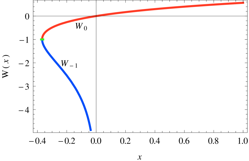
Since the mapping in Eq. (1) is not injective, no unique inverse of the $x\,e^{x}$ function exists (except at the minimum). As can be seen in Fig. 1, the Lambert W function has two real branches with a branching point located at $(-e^{-1},\,-1)$. The bottom branch, $\operatorname{W}_{-1}(x)$, is defined in the interval $x\in[-e^{-1},\,0]$ and has a negative singularity for $x\to 0^{-}$. The upper branch $\operatorname{W}_{0}(x)$ is defined for $x\in[-e^{-1},\,\infty]$.

The earliest mention of the problem of Eq. (2) is attributed to Euler [2]. However, Euler himself credited Lambert for his previous work in this subject, Lambert’s transcendental equation [3]. The $\operatorname{W}(x)$ function started to be named after Lambert only recently, in the last 20 years or so; nevertheless, the first usage of the letter $\operatorname{W}$ appeared much earlier [4].

Recently, the $\operatorname{W}(x)$ function amassed quite a following in the mathematical community [5]. Its most faithful proponents are suggesting elevating it among the present set of elementary functions, such as $\sin(x)$, $\cos(x)$, $\exp(x)$, $\ln(x)$, etc. The main argument for doing so is the fact that W is the root of the simplest exponential polynomial function given in Eq. (2). We will acknowledge these efforts by strict usage of a roman symbol W as its name.

Figure 1: The two branches of the Lambert W function, $\operatorname{W}_{-1}(x)$ in blue and $\operatorname{W}_{0}(x)$ in red. The branching point at $(-e^{-1},\,-1)$ is indicated with a green dash.

While the Lambert W function is called LambertW in the mathematics software tool Maple [6] and lambertw in the Matlab programming environment [7], in the Mathematica computer algebra framework this function [8] is implemented under the name ProductLog (in the recent versions an alias LambertW is also supported). In open source format the Lambert W function is available in the special-functions part of the GNU Scientific Library (GSL) [9], unfortunately implemented using only the slower Halley’s iteration (see discussion in Section 6).

There are numerous, well documented applications of $\operatorname{W}(x)$, certainly abundant in mathematics (like linear delay-differential equations [10]), numerics [11], computer science [12] and engineering [13], but surprisingly many also in physics, just to mention a few (without preference): quantum mechanics (solutions for double-well Dirac-delta potentials [14]), quantum statistics [15], general relativity (solutions to (1+1)-gravity problem [16], inverse of Eddington-Finkelstein (tortoise) coordinates [17]), statistical mechanics [18], fluid dynamics [19], optics [20] etc.

The main motivation for the implementation in this work comes from the research in cosmic ray physics where it has been in use already for several years [21] and new interesting applications are appearing frequently [22]. In the next sections let us describe two new examples that arise from this field of astrophysics.

1.1 Inverse of the Moyal function

Figure 2: Top: The Moyal function $\operatorname{M}(x)$. Bottom: A family of one-parametric Gaisser-Hillas functions $g(x;\,x_{\text{max}})$ for $x_{\text{max}}$ in the range from 1 to 10 with step 1.

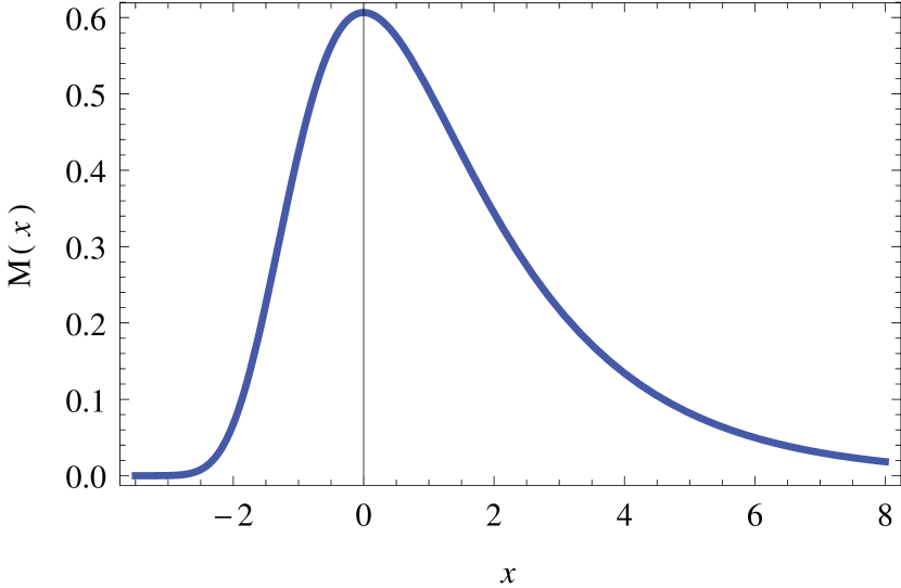
The Moyal function and the related distribution was proposed as a good approximation for the more complicated Landau distribution [23] used in descriptions of energy loss of charged particles passing through matter [24]. The un-normalized Moyal function is defined as

$$\operatorname{M}(x)=\exp\left[-\tfrac{1}{2}\left(x+e^{-x}\right)\right]$$ (5)

and can be seen in Fig. 2 (top).

Its inverse can be written in terms of the two branches of the Lambert W function,

$$\operatorname{M}^{-1}_{\pm}(x)=\operatorname{W}_{0,-1}(-x^{2})-2\ln x.$$ (6)

In experimental astrophysics the Moyal function is used for phenomenological recovery of the saturated signals from photomultipliers [25], where the largest parts of the saturated signals are obscured by the limited range of the analog-to-digital converters.

1.2 Inverse of the Gaisser-Hillas function

In astrophysics the Gaisser-Hillas function is used to model the longitudinal particle density in a cosmic-ray air shower [26]. We can show that the inverse of the three-parametric Gaisser-Hillas function,

$$G(X;\,X_{0},X_{\text{max}},\lambda)=\left[\frac{X-X_{0}}{X_{\text{max}}-X_{0}}\right]^{\frac{X_{\text{max}}-X_{0}}{\lambda}}\exp\left(\frac{X_{\text{max}}-X}{\lambda}\right),$$ (7)

is intimately related to the Lambert W function. Using rescale substitutions,

$$x=\frac{X-X_{0}}{\lambda}\qquad\text{and}\qquad x_{\text{max}}=\frac{X_{\text{max}}-X_{0}}{\lambda},$$ (8)

the Gaisser-Hillas function is modified into a function of one parameter only,

$$g(x;\,x_{\text{max}})=\left[\frac{x}{x_{\text{max}}}\right]^{x_{\text{max}}}\exp(x_{\text{max}}-x).$$ (9)

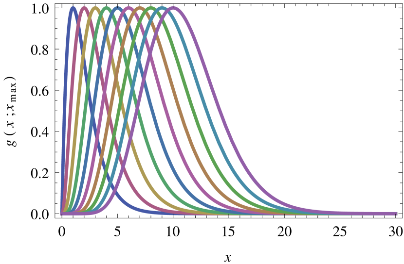
The family of one-parametric Gaisser-Hillas functions is shown in Fig. 2 (bottom). The problem of finding an inverse,

$$g(x;\,x_{\text{max}})\equiv y$$ (10)

for $0<y\leqslant 1$, can be rewritten into

$$-\frac{x}{x_{\text{max}}}\exp\left(-\frac{x}{x_{\text{max}}}\right)=-y^{1/x_{\text{max}}}\,e^{-1}.$$ (11)

According to the definition (2), the two (real) solutions for $x$ are obtained from the two branches of the Lambert W function,

$$x_{1,2}=-x_{\text{max}}\operatorname{W}_{0,-1}(-y^{1/x_{\text{max}}}\,e^{-1}).$$ (12)

Note that the branch $-1$ or $0$ simply chooses the right or left side relative to the maximum, respectively.

The Gaisser-Hillas function is intimately related to the gamma distribution which was successfully used somewhat earlier [27] in an approximate description of the mean longitudinal profile of the energy deposition in electromagnetic cascades. It is trivial to show that the inverses of the gamma and inverse-gamma distributions [28] are expressible in terms of the Lambert W function as well.

2 Numerical methods

Before describing the actual implementation let us review some of the possible numerical and analytical approaches to find $\operatorname{W}(x)$.

2.1 Recursion

For $x>0$ and $\operatorname{W}(x)>0$ we can take the natural logarithm of Eq. (4) and rearrange it into

$$\operatorname{W}(x)=\ln x-\ln\operatorname{W}(x).$$ (13)

From here it is clear that an analytical expression for $\operatorname{W}(x)$ will exhibit a certain degree of self similarity. The $\operatorname{W}(x)$ function has multiple branches in the complex domain. Due to the $x>0$ and $\operatorname{W}(x)>0$ conditions, Eq. (13) represents the positive part of the $\operatorname{W}_{0}(x)$ principal branch and in this form it is suitable for evaluation when $\operatorname{W}_{0}(x)>1$, i.e. when $x>e$.

Unrolling the self-similarity in Eq. (13) as a recursive relation, the following curious expression for $\operatorname{W}_{0}(x)$ is obtained,

$$\operatorname{W}_{0}(x)=\ln x-\ln(\ln x-\ln(\ln x-\,\ldots\,)),$$ (14)

or in the shorthand of a continued logarithm,

$$\operatorname{W}_{0}(x)=\ln\frac{x}{\ln\frac{x}{\ln\frac{x}{\cdots}}}.$$ (15)

The above expression clearly has the form of successive approximations, the final result given by the limit, if it exists.

For $x<0$ and $\operatorname{W}(x)<0$ we can multiply both sides of Eq. (4) with $-1$, take logarithm, and rewrite it into a similar expansion for the $\operatorname{W}_{-1}(x)$ branch,

$$\operatorname{W}(x)=\ln(-x)-\ln(-\operatorname{W}(x)).$$ (16)

Again, this leads to the similar recursion,

$$\operatorname{W}_{-1}(x)=\ln(-x)-\ln(-(\ln(-x)-\ln(-\ldots))),$$ (17)

or as a continued logarithm,

$$\operatorname{W}_{-1}(x)=\ln\frac{-x}{-\ln\frac{-x}{-\ln\frac{-x}{\cdots}}}.$$ (18)

For this continued logarithm we will use the symbol $R_{-1}^{[n]}(x)$ where $n$ denotes the depth of the recursion in Eq. (18).

Starting from yet another rearrangement of Eq. (4),

$$\operatorname{W}(x)=\frac{x}{\exp\operatorname{W}(x)},$$ (19)

we can obtain a recursion relation for the $-e^{-1}<x<e$ part of the principal branch $\operatorname{W}_{0}(x)<1$,

$$\operatorname{W}_{0}(x)=\frac{x}{\exp\frac{x}{\exp\frac{x}{\ldots}}}.$$ (20)

2.2 Halley’s iteration

We can apply Halley’s root-finding method [29] to derive an iteration scheme for $f(y)=W(y)-x$ by writing the second-order Taylor series

$$f(y)=f(y_{n})+f^{\prime}(y_{n})\,(y-y_{n})+\tfrac{1}{2}f^{\prime\prime}(y_{n})\,(y-y_{n})^{2}+\cdots$$ (21)

Since root $y$ of $f(y)$ satisfies $f(y)=0$ we can approximate the left-hand side of Eq. (21) with 0 and replace $y$ with $y_{n+1}$. Rewriting the obtained result into

$$y_{n+1}=y_{n}-\frac{f(y_{n})}{f^{\prime}(y_{n})+\tfrac{1}{2}f^{\prime\prime}(y_{n})\,(y_{n+1}-y_{n})}$$ (22)

and using Newton’s method $y_{n+1}-y_{n}=-f(y_{n})/f^{\prime\prime}(y_{n})$ on the last bracket, we arrive at the expression for Halley’s iteration for the Lambert W function

$$W_{n+1}=W_{n}+\frac{t_{n}}{t_{n}\,s_{n}-u_{n}},$$ (23)

where

$$t_{n} =W_{n}\,e^{W_{n}}-x,$$ (24)

$$s_{n} =\frac{W_{n}+2}{2(W_{n}+1)},$$ (25)

$$u_{n} =(W_{n}+1)\,e^{W_{n}}.$$ (26)

This method is of the third order, i.e. having $W_{n}=\operatorname{W}(x)+\mathcal{O}(\varepsilon)$ will produce $W_{n+1}=\operatorname{W}(x)+\mathcal{O}(\varepsilon^{3})$. Supplying this iteration with a sufficiently accurate first approximation of the order of $\mathcal{O}(10^{-4})$ will thus give a machine-size floating point precision $\mathcal{O}(10^{-16})$ in at least two iterations.

2.3 Fritsch’s iteration

For both branches of the Lambert W function a more efficient iteration scheme exists [30],

$$W_{n+1}=W_{n}(1+\varepsilon_{n}),$$ (27)

where $\varepsilon_{n}$ is the relative difference of successive approximations at iteration $n$,

$$\varepsilon_{n}=\frac{W_{n+1}-W_{n}}{W_{n}}.$$ (28)

The relative difference can be expressed as

$$\varepsilon_{n}=\left(\frac{z_{n}}{1+W_{n}}\right)\left(\frac{q_{n}-z_{n}}{q_{n}-2z_{n}}\right),$$ (29)

where

$$z_{n} =\ln\frac{x}{W_{n}}-W_{n},$$ (30)

$$q_{n} =2(1+W_{n})\left(1+W_{n}+\tfrac{2}{3}z_{n}\right).$$ (31)

The error term in this iteration is of a fourth order, i.e. with $W_{n}=\operatorname{W}(x)+\mathcal{O}(\varepsilon_{n})$ we obtain $W_{n+1}=\operatorname{W}(x)+\mathcal{O}(\varepsilon_{n}^{4})$.

Supplying this iteration with a sufficiently reasonable first guess, accurate to the order of $\mathcal{O}(10^{-4})$, will therefore deliver machine-size floating point precision $\mathcal{O}(10^{-16})$ in only one iteration and excessive $\mathcal{O}(10^{-64})$ in two! The main goal now is to find reliable first order approximations that can be fed into Fritsch’s iteration. Due to the lively landscape of the Lambert W function properties, the approximations will have to be found in all the particular ranges of the function’s behavior.

3 Initial approximations

The following section deals with finding the appropriate initial approximations in the whole definition range of the two branches of the Lambert W function.

3.1 Branch-point expansion

Figure 3: Successive orders of the branch-point expansion for $\operatorname{W}_{-1}(x)$ on the top and $\operatorname{W}_{0}(x)$ on the bottom.

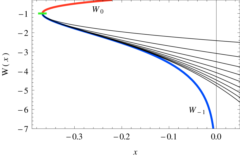
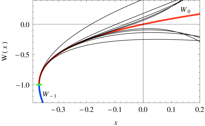
The inverse of the Lambert W function, $\operatorname{W}^{-1}(y)=y\,e^{y}$, has two extrema located at $\operatorname{W}^{-1}(-1)=-e^{-1}$ and $\operatorname{W}^{-1}(-\infty)=0^{-}$. Expanding $\operatorname{W}^{-1}(y)$ to the second order around the minimum at $y=-1$ we obtain

$$\operatorname{W}^{-1}(y)\approx-\frac{1}{e}+\frac{(y+1)^{2}}{2e}.$$ (32)

The inverse $\operatorname{W}^{-1}(y)$ is thus approximated in the lowest order by a parabolic term implying that the Lambert W function will have square-root behavior in the vicinity of the branch point $x=-e^{-1}$,

$$\operatorname{W}_{-1,0}(x)\approx-1\mp\sqrt{2(1+ex)}.$$ (33)

To obtain the additional terms in Eq. (33) we proceed by defining an inverse function, centered and rescaled around the minimum, i.e. $f(y)=2(e\operatorname{W}^{-1}(y-1)+1)$. Due to this centering and rescaling, the Taylor series around $y=0$ becomes particularly neat,

$$f(y)=y^{2}+\tfrac{2}{3}y^{3}+\tfrac{1}{4}y^{4}+\tfrac{1}{15}y^{5}+\cdots$$ (34)

Using this expansion we can derive coefficients [31] of the corresponding inverse function

$$f^{-1}(z) =1+\operatorname{W}\left(\frac{z-2}{2e}\right)=$$ (35)

$$=z^{1/2}-\tfrac{1}{3}z+\tfrac{11}{72}z^{3/2}-\tfrac{43}{540}z^{2}+\cdots$$ (36)

From Eq. (35) we see that $z=2(1+ex)$. Using $p_{\pm}(x)=\pm\sqrt{2(1+ex)}$ as an independent variable we can write this series expansion as

$$\operatorname{W}_{-1,0}(x)\approx B_{-1,0}^{[n]}(x)=\sum_{i=0}^{n}b_{i}p_{\mp}^{i}(x),$$ (37)

where the lowest few coefficients $b_{i}$ are

$i$	0	1	2	3	4	5	6	7
$b_{i}$	-1	1	$-\tfrac{1}{3}$	$\tfrac{11}{72}$	$-\tfrac{43}{540}$	$\tfrac{769}{17\,280}$	$-\tfrac{221}{8\,505}$	$\tfrac{680\,863}{43\,545\,600}$

and more of them are given in the accompanying code (see Fig. 3 for succesive orders of the series).

3.2 Asymptotic series

Another useful tool is the asymptotic expansion [32]. Using

$$A(a,b)=a-b+\sum_{k}\sum_{m}C_{km}a^{-k-m-1}b^{m+1},$$ (38)

with $C_{km}$ related to the Stirling numbers of the first kind, the Lambert W function can be expressed as

$$\operatorname{W}_{-1,0}(x)=A(\ln(\mp x),\,\ln(\mp\ln(\mp x))),$$ (39)

with $a=\ln x$, $b=\ln\ln x$ for the $\operatorname{W}_{0}$ branch and $a=\ln(-x)$, $b=\ln(-\ln(-x))$ for the $\operatorname{W}_{-1}$ branch. The first few terms are

$$A(a,b) =a-b+\frac{b}{a}+\frac{b(-2+b)}{2a^{2}}+\frac{b(6-9b+2b^{2})}{6a^{3}}+$$

$$\,+\frac{b(-12+36b-22b^{2}+3b^{3})}{12a^{4}}+$$ (40)

$$\,+\frac{b(60-300b+350b^{2}-125b^{3}+12b^{4})}{60a^{5}}+\cdots$$

3.3 Rational fits

A useful quick-and-dirty approach to the functional approximation is to generate a large enough sample of data points $\{w_{i}\,e^{w_{i}},\,w_{i}\}$, which evidently lie on the Lambert W function. Within some appropriately chosen range of $w_{i}$ values, the points are fitted with a rational approximation

$$Q(x)=\frac{\sum_{i}a_{i}x^{i}}{\sum_{i}b_{i}x^{i}},$$ (41)

varying the order of the polynomials in the nominator and denominator, and choosing the one that has the lowest maximal absolute residual in a particular interval of interest.

For the $\operatorname{W}_{0}(x)$ branch, the first set of equally-spaced $w_{i}$ components was chosen in a range that produced $w_{i}\,e^{w_{i}}$ values in an interval $[-0.3,\,0]$. The optimal rational fit turned out to be

$$Q_{0}(x)=x\frac{1+a_{1}x+a_{2}x^{2}+a_{3}x^{3}+a_{4}x^{4}}{1+b_{1}x+b_{2}x^{2}+b_{3}x^{3}+b_{4}x^{4}}$$ (42)

where the coefficients for this first approximation $Q_{0}^{[1]}(x)$ are

$i$	1	2	3	4
$a_{i}$	5.931375’	11.392205’	07.338883’	0.653449’
$b_{i}$	6.931373’	16.823494’	16.430723’	5.115235’

For the second fit of the $\operatorname{W}_{0}(x)$ branch a $w_{i}$ range was chosen so that the $w_{i}\,e^{w_{i}}$ values were produced in the interval $[0.3,\,2e]$, giving rise to the second optimal rational fit $Q_{0}^{[2]}(x)$ of the same form as in Eq. (42) but with coefficients

$i$	1	2	3	4
$a_{i}$	2.445053’	1.343664’	0.148440’	0.000804’
$b_{i}$	3.444708’	3.292489’	0.916460’	0.053068’

For the $\operatorname{W}_{-1}(x)$ branch a single rational approximation of the form

$$Q_{-1}(x)=\frac{a_{0}+a_{1}x+a_{2}x^{2}}{1+b_{1}x+b_{2}x^{2}+b_{3}x^{3}+b_{4}x^{4}+b_{5}x^{5}}$$ (43)

with the coefficients

$i$	0	1	2
$a_{i}$	-7.814176’	253.888101’	657.949317’
$b_{i}$		-60.439587’	99.985670’
$i$	3	4	5
$b_{i}$	682.607399’	962.178439’	1477.934128’

is enough.

4 Implementation

To quantify the accuracy of a particular approximation $\widetilde{\operatorname{W}}(x)$ of the Lambert function $\operatorname{W}(x)$ we can introduce a quantity $\Delta(x)$ defined as

$$\Delta(x)=\log_{10}|\operatorname{W}(x)|-\log_{10}|\widetilde{\operatorname{W}}(x)-\operatorname{W}(x)|,$$ (44)

so that it gives us a number of correct decimal places the approximation $\widetilde{\operatorname{W}}(x)$ is producing for some value of the parameter $x$.

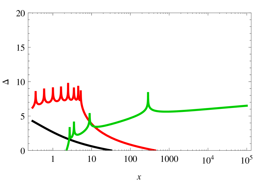
In Fig. 4 all approximations for the $\operatorname{W}_{0}(x)$ mentioned above are shown in the linear interval $[-e^{-1},\,0.3]$ on the left and the logarithmic interval $[0.3,\,10^{5}]$ on the right. For each of the approximations an optimal interval is chosen so that the number of accurate decimal places is maximized over the whole definition range. For the $\operatorname{W}_{0}(x)$ branch the resulting piecewise approximation

$$\widetilde{\operatorname{W}}_{0}(x)=\begin{cases}B_{0}^{[9]}(x)&;\,-e^{-1}\leqslant x<a\\ Q_{0}^{[1]}(x)&;\,a\leqslant x<b\\ Q_{0}^{[2]}(x)&;\,b\leqslant x<c\\ A_{0}(x)&;\,c\leqslant x<\infty\end{cases}$$ (45)

with $a=-0.323581^{\prime}$, $b=0.145469^{\prime}$, and $c=8.706658^{\prime}$, is accurate in the definition range $[-e^{-1},\,7]$ to at least 5 decimal places and to at least 3 decimal places in the whole definition range $[-e^{-1},\,\infty]$. Note that $B_{0}^{[9]}(x)$ comes from Eq. (37), $Q_{0}^{[1]}(x)$ and $Q_{0}^{[2]}(x)$ are from Eq. (42), and $A_{0}(x)$ is from Eq. (40).

Figure 4: Combining different approximations of $\operatorname{W}_{0}(x)$ into a final piecewise function. The number of accurate decimal places $\Delta(x)$ is shown for two ranges, linear interval $[-e^{-1},\,0.3]$ (top) and logarithmic interval $[0.3,\,10^{5}]$ (bottom). The approximations are branch-point expansion $B_{0}^{[9]}(x)$ from Eq. (37) (blue), rational fits $Q_{0}^{[1]}(x)$ and $Q_{0}^{[2]}(x)$ from Eq. (42) in black and red, respectively, and asymptotic series $A_{0}(x)$ from Eq. (40) (green).

Figure 5: Final values of the combined approximation $\widetilde{\operatorname{W}}_{0}(x)$ (black) from Fig. 4 after one step of Halley’s iteration (red) and one step of Fritsch’s iteration (blue).

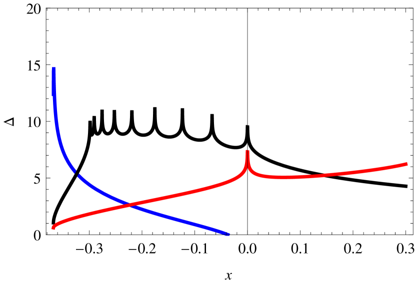
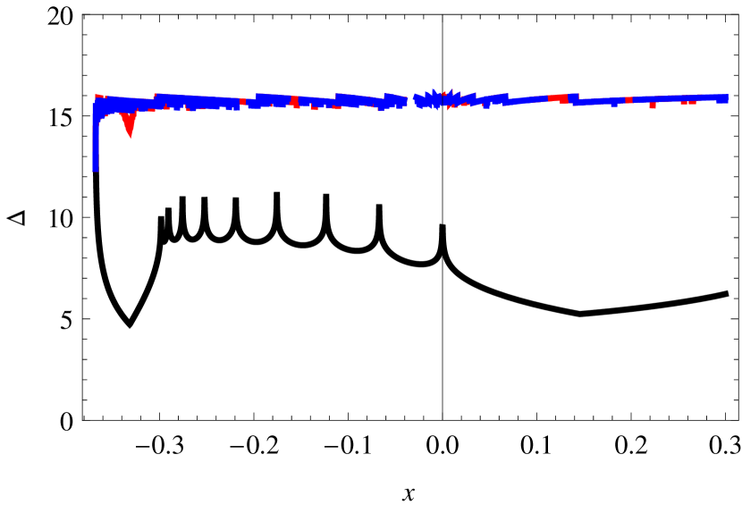
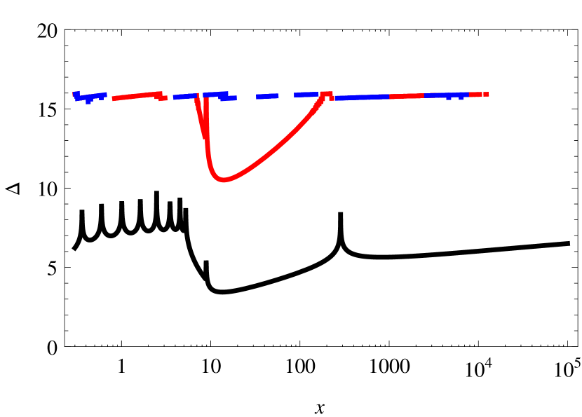
The accuracy of the final piecewise approximation $\widetilde{\operatorname{W}}_{0}(x)$ is shown in Fig. 5 (black line). Using this approximation, a single step of Halley’s iteration (red) and Fritsch’s iteration (blue) is performed and the resulting number of accurate decimal places is shown. As can be seen from the plots, both iterations produce machine-size accurate floating point numbers in the whole definition interval except for the interval between 6.5 and 190 where the Halley’s method requires another step of the iteration. For that reason we have decided to use only (one step of) Fritsch’s iteration in the C++ implementation of the Lambert W function.

Figure 6: Top: Approximations of the $\operatorname{W}_{-1}(x)$ branch. The branch-point expansion $B_{-1}^{[9]}(x)$ is shown in blue, the rational approximation $Q_{-1}(x)$ in black, and the logarithmic recursion $R_{-1}^{[9]}$ in red. Bottom: The combined approximation is accurate to at least 5 decimal places in the whole definition range. The results after applying one step of Halley’s iteration are shown in red and after one step of Fritsch’s iteration in blue.

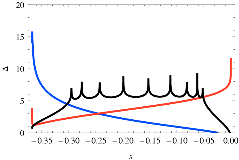
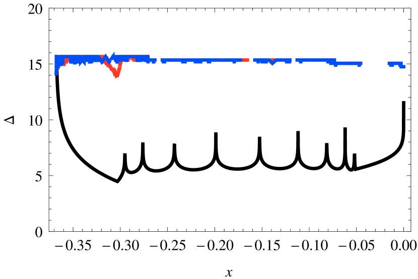
In Fig. 6 (top) the same procedure is shown for the $\operatorname{W}_{-1}(x)$ branch. The final approximation

$$\widetilde{\operatorname{W}}_{-1}(x)=\begin{cases}B_{-1}^{[9]}(x)&;\,-e^{-1}\leqslant x<a\\ Q_{-1}(x)&;\,a\leqslant x<b\\ R_{-1}^{[9]}(x)&;\,b\leqslant x<0\end{cases}$$ (46)

with $a=-0.302985^{\prime}$ and $b=-0.051012^{\prime}$, is accurate to at least 5 decimal places in the whole definition range $[-e^{-1},\,0]$. Note that $B_{-1}^{[9]}(x)$ is taken from Eq. (37), $Q_{-1}(x)$ is from Eq. (43), and $R_{-1}^{[9]}(x)$ is from Eq. (18).

In Fig. 6 (bottom) the combined approximation $\widetilde{\operatorname{W}}_{-1}(x)$ is shown (black line). The values after one step of Halley’s iteration are shown in red and after one step of Fritsch’s iteration in blue. Similarly as for the previous branch, Fritsch’s iteration turns out to be superior, yielding machine-size accurate results in the whole definition range, while Halley’s iteration is accurate to at least 13 decimal places.

5 Source availability, installation and usage

The most recent version of the sources of this implementation with some additional material and examples are available from
https://github.com/DarkoVeberic/LambertW
and are released under the dual GPL/BSD license.

Apart from the special functions in GSL [9], this is the only freely available implementation of the Lambert W function in C++ and to the best of our knowledge the only implementation using the superior Fritsch’s version of the iteration.

The supplied C++ code implements the following set of functions

• double LambertWApproximation<$b$>(double x);

• double LambertW<$b$>(double x);

• double LambertW(int branch, double x);

where $b$ in the first two functions should be replaced with the compile-time branch integer value, e.g. LambertW<-1>(x) or LambertW<0>(x). Apart from the slightly increased efficiency, the main reason for implementing the first two functions with the branch $b$ as a compile time parameter is to force the users to think about the two possible solutions to the problem in Eq. (2). Just as for solutions to the quadratic equation where the $\pm$ sign has to be chosen based on the desired solution, the Lambert W function offers two possibilities that need careful consideration.

The initial approximations $\widetilde{\operatorname{W}}_{b}(x)$ from Eqs. (46) and (45), that are used to kick-start the iterations, are also directly available as LambertWApproximation<$b$>(x), as they might be useful in applications for which it is sufficient to have a limited number of accurate decimal places (see the discussion above).

The supplied code does not need any kind of special installation procedures. In the case that your analysis needs an evaluation of the Lambert W function, the two source files, LambertW.h and LambertW.cc, should be simply bundled with your project structure and compiled with a suitable C++ compiler.

The source distribution also includes a command-line utility implemented by the lambert-w.cc source file. The included Makefile can, with the request make lambert-w, build an executable command. It can be invoked through a shell as ./lambert-w [branch] x, taking an optional branch number (0 by default) and a parameter x. The output of the command is equivalent to the $\operatorname{W}_{\texttt{branch}}(\texttt{x})$ return value and can thus be simply used in shell scripts (sh, bash, or csh) or other programming languages with easy access to shell invocations (awk, perl etc.).

Also included in the distribution is a test suite which can perform a correctness check on your build by comparing obtained and expected return values of the Lambert W function on your system. It is invoked by the command make tests. Any potential discrepancies larger than the double machine precision ($\gtrsim 10^{-14}$) will be reported in the output.

6 Timing

Figure 7: Execution speedup $t^{\prime}_{\text{gsl}}/t^{\prime}$, relative to the GSL implementation [9] for the $\operatorname{W}_{0}(x)$ branch (red) and the $\operatorname{W}_{-1}(x)$ branch (blue). For $x>2$ the ratio slowly decreases and is $\sim 2$ for $x>8$. Time of the respective driver loops and function calls was subtracted in order to measure only differences between the pure numerical parts of the two implementations (see text for details).

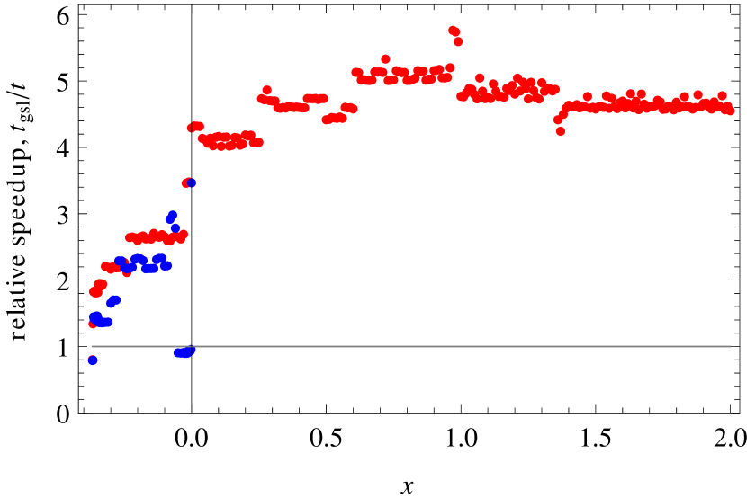
We have decided to compare the execution time of our code relative to the GNU GSL library (implemented in the C language) since comparisons to interpreted code (like Maple, Matlab or Mathematica) would, besides common availability problems, not be fair in terms of speed.

In Fig. 7 relative speedup, $t_{\text{gsl}}/t$, is shown as a function of the Lambert W parameter $x$. Timing accuracy of several % was achieved by running 3 000 000 function calls in a loop, taking special care that the compiler did not optimize code away by slightly modifying $x$ on each call and then gathering all results into a summed variable reported at the end. For each of the two implementations an identical code was also run with the Lambert W function call replaced with a simple identity function (just returning its input parameter) in order to estimate the overhead of the surrounding timing code. This $t_{\text{overhead}}$ is then consequently subtracted from the time of the Lambert W runs $t$, giving an approximation to the time taken by the pure function call, $t^{\prime}=t-t_{\text{overhead}}$. The ratio $t^{\prime}_{\text{gsl}}/t^{\prime}$ is then plotted in Fig. 7.

As can be clearly seen from Fig. 7, our implementation is at least $2\times$ faster than GSL for a broad range of input parameters $x$, but the largest efficiency gains (up to $5\times$) are observed in the ranges where rational fits $Q_{b}$ from Eqs. (45) and (46) are used. Although Fritsch’s iteration is in general more complex than Halley’s, at the end it pays off, yielding machine-size accuracy with a single step where Halley’s might need more, also due to poor initial approximations used in GSL. GSL performs better only in the small regions where branch-point and asymptotic expansions are used without the consequent Halley’s iteration refinements. The comparisons were made on the Ubuntu 12.04 x86_64 Linux operating system running on a 2.2 GHz AMD Opteron 275 processor, using the GCC 4.6.3 compiler with optimization option -O2.

7 Conclusions

We have shown that Fritsch’s iteration scheme coupled with accurate initial approximations can deliver significant efficiency gains in the numerical evaluation of the real branches of the Lambert W function. The open-source release of our C++ implementation is suitable for inclusion in various analysis packages used in all fields of physics.

References

- [1]
- [2] L. Euler, Acta Acad. Scient. Petropol. 2 (1783) 29--51.
- [3] J.H. Lambert, Acta Helvitica 3 (1758) 128--168.
- [4] G. Pólya and G. Szegö, Aufgaben und Lehrsätze aus der Analysis, J. Springer, Berlin, 1925.
- [5] http://www.orcca.on.ca/LambertW/.
- [6] R.M. Corless, G.H. Gonnet, D.E.G. Hare, and D.J. Jeffrey, Maple Technical Newsletter 9 (1993) 12.
-
[7]
http://www.mathworks.com/help/toolbox/symbolic/
lambertw.html; some open source versions for Matlab: P. Getreuer and D. Clamond, http://www.getreuer.info/home/
lambertw; N.N. Schraudolph and D. Ross, http://www.cs.toronto.edu/~dross/code/LambertW.m. - [8] E.W. Weisstein, Lambert W-Function, MathWorld Wolfram Web Resource, http://mathworld.wolfram.com/LambertW-Function.html.
- [9] G. Jungman and K. Briggs, GNU Scientific Library, gsl-1.15, specfunc/lambert.c, http://www.gnu.org/software/gsl/.
- [10] F.M. Asl and A.G. Ulsoy, J. Dyn. Sys. Meas. Control 125 (2003) 215; S. Yi, P.W. Nelson, and A.G. Ulsoy, IEEE Trans. Autom. Control 53 (2008) 854--860.
- [11] R.M. Corless, G.H. Gonnet, D.E.G. Hare, D.J. Jeffrey, and D.E. Knuth, Adv. Comput. Math. 5 (1996) 329; R.M. Corless, D.J. Jeffrey, and D.E. Knuth, 1997, A Sequence of Series for the Lambert Function, in: Proc. ISSAC ’97, Maui, (1997) 197--204; R.M. Corless and D.J. Jeffrey, The Wright function, in: J. Calmet, B. Benhamou, O. Caprotti, L. Henocque, V. Sorge (Eds.), Artificial Intelligence, Automated Reasoning, and Symbolic Computation, in: Proc. AISC-Calculemus 2002, Springer (2002) 76--89.
- [12] J. Bustos-Jimenez, N. Bersano, S.E. Schaeffer, J.M. Piquer, A. Iosup, and A. Ciuffoletti, in Grid Computing: Achievements and Prospects, eds. S. Gorlatch, P. Fragopoulou, and T. Priol, Springer (2008); doi:10.1007/978-0-387-09457-1_6.
- [13] S. Yi, P.W. Nelson, and A.G. Ulsoy, Math. Biosci. Engrg. 4 (2007) 355--368.
- [14] T.C. Scott, M. Aubert-Frécon, and J. Grotendorst, Chem. Phys. 324 (2006) 323--338; T.C. Scott, A. Lüchow, D. Bressanini, and J.D. Morgan III, Phys. Rev. A 75 (2007) 060101R; T.C. Scott, J.F. Babb, A. Dalgamo, and J.D. Morgan III, Chem. Phys. Lett. 203 (1993) 175--183.
- [15] S.R. Valluri, M. Gil, D.J. Jeffrey, and S. Basu, J. Math. Phys. 50 (2009) 102103.
- [16] T.C. Scott, R. Mann, and R.E. Martinez II, Appl. Algebra Engrg. Comm. Comput. 17 (2006) 41--47.
- [17] A.S. Eddington, Nature 113 (1924) 192; T. Regge and J.A. Wheeler, Phys. Rev. 108 (1957) 1063--1069.
- [18] J.-M. Caillol, J. Phys. A 36 (2003) 10431--10442.
- [19] S.P. Pudasaini, Phys. Fluids 23 (2011) 043301.
- [20] O. Steinvall, Appl. Optics 48 (2009) B1--B7.
- [21] S. Argirò et al., Nucl. Instr. and Meth. A 580 (2007) 1485.
- [22] K.-H. Kampert and M. Unger, Astropart. Phys. 35 (2012) 660--678; arXiv:1201.0018.
- [23] J.E. Moyal, Phil. Mag. 46 (1955) 263.
- [24] L.D. Landau, J. Phys. USSR 8 (1944) 201--205.
- [25] I.C. Mariş, M. Roth, and T. Schmidt, A Phenomenological Method to Recover the Signal from Saturated Stations, P. Auger Collaboration internal note GAP-2006-012.
- [26] T.K. Gaisser and A.M. Hillas, Proc. of the 15th Internation Cosmic-Ray Conference, Plavdiv, 8 (1977) 353.
- [27] E. Longo and I. Sestili, Nucl. Instrum. Methods 128 (1975) 283.
- [28] C. Walck, Hand-book on statistical distributions for experimentalists, Stockholms Universitet, Internal Report SUF-PFY/96-01, 10 September 2007, pp. 69--74.
- [29] T.R. Scavo and J.B. Thoo, Amer. Math. Monthly 102 (1995) 417.
- [30] F.N. Fritsch, R.E. Shafer, and W.P. Crowley, Commun. ACM 16 (1973) 123.
- [31] P.M. Morse and H. Feshbach, Methods of Theoretical Physics, Part I, McGraw-Hill, New York (1953) 411.
- [32] N.G. de Bruijn, Asymptotic Methods in Analysis, New York, Dover (1981) 27.