Matrices commuting with a given normal tropical matrix

Abstract

Consider the space $M_{n}^{nor}$ of square normal matrices $X=(x_{ij})$ over $\mathbb{R}\cup\{-\infty\}$, i.e., $-\infty\leq x_{ij}\leq 0$ and $x_{ii}=0$. Endow $M_{n}^{nor}$ with the tropical sum $\oplus$ and multiplication $\odot$. Fix a real matrix $A\in M_{n}^{nor}$ and consider the set $\Omega(A)$ of matrices in $M_{n}^{nor}$ which commute with $A$. We prove that $\Omega(A)$ is a finite union of alcoved polytopes; in particular, $\Omega(A)$ is a finite union of convex sets. The set $\Omega^{A}(A)$ of $X$ such that $A\odot X=X\odot A=A$ is also a finite union of alcoved polytopes. The same is true for the set $\Omega^{\prime}(A)$ of $X$ such that $A\odot X=X\odot A=X$.

A topology is given to $M_{n}^{nor}$. Then, the set $\Omega^{A}(A)$ is a neighborhood of the identity matrix $I$. If $A$ is strictly normal, then $\Omega^{\prime}(A)$ is a neighborhood of the zero matrix. In one case, $\Omega(A)$ is a neighborhood of $A$. We give an upper bound for the dimension of $\Omega^{\prime}(A)$. We explore the relationship between the polyhedral complexes $\operatorname{span}A$, $\operatorname{span}X$ and $\operatorname{span}(AX)$, when $A$ and $X$ commute. Two matrices, denoted $\underline{A}$ and $\overline{A}$, arise from $A$, in connection with $\Omega(A)$. The geometric meaning of them is given in detail, for one example. We produce examples of matrices which commute, in any dimension.

AMS class.: 15A80; 14T05.

Keywords and phrases: tropical algebra, commuting matrices, normal matrix, idempotent matrix, alcoved polytope, convexity.

1 Introduction

Let $n\in\mathbb{N}$ and $K$ be a field. Fix a matrix $A\in M_{n}(K)$ and consider $K[A]$, the algebra of polynomial expressions in $A$. In classical mathematics, the set $\Omega(A)$ of matrices commuting with $A$ is well–known: $\Omega(A)$ equals $K[A]$ if and only if the characteristic and minimal polynomials of $A$ coincide. Otherwise, $K[A]$ is a proper linear subspace of $\Omega(A)$; see [27], chap. VII.

In this paper we study the analogous of $\Omega(A)$ in the tropical setting. Moreover, we restrict ourselves to square normal matrices over $\overline{\mathbb{R}}:=\mathbb{R}\cup\{-\infty\}$, i.e., matrices $A=(a_{ij})$ with $a_{ii}=0$ and $-\infty\leq a_{ij}\leq 0$, for all $i,j$. The set of all such matrices, endowed with the tropical operations $\oplus=\max$ and $\odot=+$, is denoted $M_{n}^{nor}$.

For any $r\in\mathbb{R}_{\leq 0}$, the half–line $[-\infty,r):=\{x:-\infty\leq x<r\}$ is open in ${\overline{\mathbb{R}}}_{\leq 0}$ with the usual interval topology. A Cartesian product of such half–lines is open in ${\overline{\mathbb{R}}}^{n^{2}-n}_{\leq 0}$ with the usual product topology. The half–line $(r,0]:=\{x:r<x\leq 0\}$ is open in ${\overline{\mathbb{R}}}_{\leq 0}$. A Cartesian product of such half–lines is open in ${\overline{\mathbb{R}}}^{n^{2}-n}_{\leq 0}$.

The set $M_{n}^{nor}$ can be identified with ${\overline{\mathbb{R}}}^{n^{2}-n}_{\leq 0}$ and, via this identification, $M_{n}^{nor}$ gets a topology. Consider a matrix $X\in M_{n}^{nor}$ and a subset $V\subseteq M_{n}^{nor}$. We say that $V$ is a neighborhood of $X$ if there exists an open subset $U\subseteq M_{n}^{nor}$ such that $X\in U\subseteq V$ (we do not require $V$ to be open).

Let $\Omega(A)$ be the subset of matrices commuting with a given real matrix $A$, i.e., $X\in M_{n}^{nor}$ such that $A\odot X=X\odot A$. The tropical analog of $K[A]$ inside $M_{n}^{nor}$ is the set $\mathcal{P}(A)$ of tropical powers of $A$. In general, $\Omega(A)$ is larger than $\mathcal{P}(A)$ (see proposition 1).

Our new results are gathered in sections 3, 18 and 5. In section 3 we prove that

$$\Omega(A)=\bigcup_{w}\Omega_{w}(A)$$

is a finite union of alcoved polytopes, (see corollary 5). In particular, $\Omega(A)$ is a finite union of convex sets.

Two important subsets of $\Omega(A)$ are

$$\Omega^{A}(A)=\{X\in\Omega(A):X\odot A=A\odot X=A\}$$

and

$$\Omega^{\prime}(A)=\{X\in\Omega(A):X\odot A=A\odot X=X\}.$$

Both are finite unions of alcoved polytopes (see theorems 9 and 12). Moreover, $\Omega^{A}(A)$ is a neighborhood (not necessarily open) of the identity matrix $I$. If $A$ is strictly normal, then $\Omega^{\prime}(A)$ is a neighborhood of the zero matrix $0$ (see propositions 7 and 8).

The study of $\Omega^{A}(A)$ and $\Omega^{\prime}(A)$ lead us to two matrices arising from $A$, denoted $\underline{A}$ and $\overline{A}$, and we prove

$$\underline{A}\leq A\leq\overline{A},$$

(see proposition 17). Moreover, $X\leq\underline{A}$ is a necessary condition for $A\odot X=X\odot A=A$, and $\overline{A}\leq X$ is a necessary condition for $A\odot X=X\odot A=X$ (see corollary 15). This provides an upper bound for the dimension of $\Omega^{\prime}(A)$ (see corollary 16). The matrix $\underline{A}$ is explicitly given in expression (19), while the definition and computation of $\overline{A}$ is more involved (see definition 14).

In section 18 we study some instances of commutativity of matrices under perturbations. Theorem 20 is an easy way to produce two real matrices in $M_{n}^{nor}$ which commute. Another way to obtain two such matrices is given in theorem 22. The geometry is different in both instances: in the first case, the polyhedral complexes (i.e., tropical column spans) associated to the matrices are convex, but not so in the second. Under certain hypothesis we prove that $\Omega(A)$ is a neighborhood of $A$ (see corollary 21).

Section 5 has an exploratory nature. We examine the relationship among the complexes $\operatorname{span}A$, $\operatorname{span}B$, $\operatorname{span}(AB)$ and $\operatorname{span}(BA)$ when commutativity is present or absent. In addition, the geometric meaning of the matrices $\underline{A},A$ and $\overline{A}$ is given in full detail, for one example in the paper. We believe that classical convexity of $\operatorname{span}A$ depends on the matrices $\underline{A}$ and $\overline{A}$. We suspect that this is related to the question of commutativity. We leave two open questions in pages p. 18 and 3.

Alcoved polytopes play a crucial role in this paper. By definition, a polytope $\mathcal{P}$ in $\mathbb{R}^{n-1}$ is alcoved if it can be described by inequalities $c_{i}\leq x_{i}\leq b_{i}$ and $c_{ik}\leq x_{i}-x_{k}\leq b_{ik}$ , for some $i,k\in[n-1]$, $i\neq k$, and $c_{i},b_{i},c_{ik},b_{ik}\in\mathbb{R}\cup\{\pm\infty\}$. They are classically convex sets. Alcoved polytopes have been studied in [22, 23]. In connection with tropical mathematics, they appeared in [17, 18, 19, 29, 36]. Kleene stars are matrices $A$ such that $A={A}^{*}$, where $*$ is the so–called Kleene operator. Alcoved polytopes and Kleene stars are closely related notions; see [29, 32, 33].

By definition, a matrix $A=(a_{ij})$ over ${\overline{\mathbb{R}}}$ is normal if $a_{ii}=0$ and $-\infty\leq a_{ij}\leq 0$, for all $i,j$. It is strictly normal if, in addition, $-\infty\leq a_{ij}<0$, for all $i\neq j$. There are FOUR REASONS for us to restrict to normal matrices. First, it is not all too restrictive. Indeed, by the Hungarian Method (see [5, 6, 21, 26]), for every matrix $A$ there exist a (not unique) similar matrix $N$ which is normal. In practice, this means that by a relabeling of the columns of $A$ and a translation, any $A$ can be assumed to be normal. Second, normality of $A$ has a clear geometric meaning in $\mathbb{R}^{n-1}$. Consider the alcoved polytope

$$C_{A}:=\left\{x\in\mathbb{R}^{n-1}:\ {{a_{in}\leq x_{i}\leq-a_{ni}}\atop{a_{ik}\leq x_{i}-x_{k}\leq-a_{ki}}};\ 1\leq i\neq k\leq n-1\right\}.$$ (1)

Then, $A$ is normal if and only if the zero vector belongs to $C_{A}$ and the columns of the matrix $A_{0}$ (see definition in p. 4), viewed as points in $\mathbb{R}^{n-1}$, lie around the zero vector and are listed in a predetermined order (and this order is a kind of orientation in $\mathbb{R}^{n-1}$); see [29] and also [14, 15, 16]. Third, when computing examples, normal matrices are easy to handle, due to inequalities (2). Fourth and last, normal matrices satisfy many max–plus properties (e.g., they are strongly definite; see [6, 7]).

Some aspects of commutativity in tropical algebra (also called max–plus algebra or max–algebra) have been addressed earlier. It is known that two commuting matrices have a common eigenvector; see [7], sections 4.7, 5.3.5 and 9.2.2. In [20] it is proved that the critical digraphs of two commuting irreducible matrices have a common node.

2 Background and notations

For $n\in\mathbb{N}$, set $[n]:=\{1,2,\ldots,n\}$. Let $\mathbb{R}_{\leq 0}$, $\mathbb{R}_{\geq 0}$, $\overline{\mathbb{R}}_{\leq 0}$, etc. have the obvious meaning. On $\overline{\mathbb{R}}_{\leq 0}$, i.e., on the closed unbounded half–line $[-\infty,0]$, we consider the interval topology: an open set in $[-\infty,0]$ is either a finite intersection or an arbitrary union of sets of the form $[-\infty,a)$ or $(b,0]$, with $-\infty<a,b<0$.

$\oplus=\max$ is the tropical sum and $\odot=+$ is the tropical product. For instance, $3\oplus(-7)=3$ and $3\odot(-7)=-4$. Define tropical sum and product of matrices following the same rules of classical linear algebra, but replacing addition (multiplication) by tropical addition (multiplication). Consider order $n$ square matrices. The tropical multiplicative identity is $I=(\alpha_{ij})$, with $\alpha_{ii}=0$ and $\alpha_{ij}=-\infty$, for $i\neq j$. The zero matrix is denoted $0$ (every entry of it is null). We will never use classical multiplication of matrices; thus $A\odot X$ will be written $AX$, for matrices $A,X$, for simplicity.

If $A=(a_{ij})$ and $B=(b_{ij})$ are matrices of the same order, then $A\leq B$ means $a_{ij}\leq b_{ij}$, for all $i,j$.

By definition, a square matrix $A=(a_{ij})$ over ${\overline{\mathbb{R}}}$ is normal if $a_{ii}=0$ and $-\infty\leq a_{ij}\leq 0$, for all $i,j$. Thus, $A$ is normal if and only if $I\leq A\leq 0$. Let us define $A^{0}$ to be the identity matrix $I$. So we have

$$I=A^{0}\leq A\leq A^{2}\leq A^{3}\leq\cdots\leq 0$$ (2)

since tropical multiplication by any matrix is monotonic (because it amounts to computing certain sums and maxima). By a theorem of Yoeli’s (see [37]), we have $A^{n-1}=A^{n}=A^{n+1}=\cdots$ and we denote this matrix by $A^{*}$ and call it the Kleene star of $A$. A matrix $A$ is a Kleene star if $A=A^{*}$.

A normal matrix $A$ is strictly normal if $a_{ij}<0$, whenever $i\neq j$.

Let $M_{n}^{nor}$ denote the family of order $n$ normal matrices over ${\overline{\mathbb{R}}}$. It is in bijective correspondence with ${\overline{\mathbb{R}}}^{n^{2}-n}_{\leq 0}$. We consider the product interval topology on ${\overline{\mathbb{R}}}^{n^{2}-n}_{\leq 0}$. The bijection carries this topology onto $M_{n}^{nor}$. The border of $M_{n}^{nor}$ is the set of matrices $A$ such that $a_{ij}=0$ or $-\infty$, for some $i\neq j$.

We will write the coordinates of points in $\mathbb{R}^{n}$ in columns. Let $A\in\mathbb{R}^{n\times m}$ and denote by $a_{1},\ldots,a_{m}\in\mathbb{R}^{n}$ the columns of $A$. The (tropical column) span of $A$ is, by definition,

$$\operatorname{span}A: =\{(\mu_{1}\odot a_{1})\oplus\cdots\oplus(\mu_{m}\odot a_{m})\in\mathbb{R}^{n}:\mu_{1},\ldots,\mu_{m}\in\mathbb{R}\}$$

$$=\max\{\mu_{1}u+a_{1},\ldots,\mu_{m}u+a_{m}:\mu_{1},\ldots,\mu_{m}\in\mathbb{R}\}$$

where $u=(1,\ldots,1)^{t}$ and maxima are computed coordinatewise. We will never use classical linear spans in this paper. Clearly, the set $\operatorname{span}A$ is closed under classical addition of the vector $\mu u$, for $\mu\in\mathbb{R}$, since $\odot=+$. Therefore, the hyperplane section $\{x_{n}=0\}\cap\operatorname{span}A$ determines $\operatorname{span}A$ completely. The set $\{x_{n}=0\}\cap\operatorname{span}A$ is a connected polyhedral complex of impure dimension $\leq n-1$ and it is not convex, in general. Let $A$ be normal. Then $\operatorname{span}A=C_{A}$ in (1) (and so it is convex) if and only if $A$ is a Kleene–star; see [29, 32]. Throughout the paper, we will identify the hyperplane $\{x_{n}=0\}$ inside $\mathbb{R}^{n}$ with $\mathbb{R}^{n-1}$. In particular, columns of order $n$ matrices having zero last row are considered as points in $\mathbb{R}^{n-1}$.

For any $d\in\mathbb{R}^{n}$, $\operatorname{diag}d$ denotes the square matrix whose diagonal is $d$ and is $-\infty$ elsewhere.

For any real matrix $A$, the matrix $A_{0}$ is defined as the tropical product

$$A\operatorname{diag}(-\operatorname{row}(A,n)).$$ (4)

Thus, the $j$–th column of $A_{0}$ is a tropical multiple of the corresponding column of $A$ (i.e., the $j$–th column of $A_{0}$ is the sum of the vector $-a_{nj}u$ and the $j$–th column of $A$). The last row of $A_{0}$ is zero. Therefore, the matrix $A_{0}$ is used to draw the complex $\{x_{n}=0\}\cap\operatorname{span}A$ inside $\mathbb{R}^{n-1}$. The sets $\operatorname{span}A$ and $\{x_{n}=0\}\cap\operatorname{span}A$ determine each other.

The simplest objects in the tropical plane $\overline{\mathbb{R}}^{2}$ are lines. Given a tropical linear form

$$p_{1}\odot X\oplus p_{2}\odot Y\oplus p_{3}=\max\{p_{1}+X,p_{2}+Y,p_{3}\}$$

a tropical line consists of the points $(x,y)^{t}$ where this maximum is attained, at least, twice. Such twice–attained–maximum condition is the tropical analog of the classical vanishing point set. Denote this line by $L_{p}$, where $p=(p_{1},p_{2},p_{3})\in\mathbb{R}^{3}$. Lines in the tropical plane are tripods. Indeed, $L_{p}$ is the union of three rays meeting at point $(p_{3}-p_{1},p_{3}-p_{2})^{t}$, in the directions west, south and north–east. The point is called the vertex of $L_{p}$.

Take $p=0$. The line $L_{0}$ splits the plane $\overline{\mathbb{R}}^{2}$ into three closed sectors $S_{1}:=\{x\geq 0,\ x\geq y\}$, $S_{2}:=\{x\leq y,\ y\geq 0\}$ and $S_{3}:=\{x\leq 0,\ y\leq 0\}$. An order 3 real matrix $A$ is normal if and only if (omitting the last row in $A_{0}$, which is zero) each column of $A_{0}$ lies in the corresponding sector i.e., $\operatorname{col}(A_{0},j)\in S_{j}$, for $j=1,2,3$. For instance, consider the normal matrix $B$ and take $B_{0}$ in example 11, figure 3 top centre, p. 11. Notice that $(5,1)^{t}\in S_{1}$, $(-3,0)^{t}\in S_{2}$ and $(-1,-6)^{t}\in S_{3}$. An analogous statement holds for $\overline{\mathbb{R}}^{n-1}$ and order $n$ matrices. See [3, 4, 11, 12, 13, 24, 25, 30] for an introduction to tropical geometry. See [1, 2, 5, 7, 8, 9, 35, 38] for an introduction to tropical (or max–plus) algebra.

3 Normal matrices which commute with $A$

The set $M_{2}^{nor}$ is commutative, since $AB=BA=A\oplus B$, for any $A,B\in M_{2}^{nor}$. Thus, we will study the set

$$\Omega(A):=\{X\in M_{n}^{nor}:AX=XA\},$$ (5)

for a real matrix $A\in M_{n}^{nor}$ and $n\geq 3$.

If $A\in M_{n}^{nor}$ is real and $\lambda\in\mathbb{R}$, then $\lambda\odot A=\lambda u+A$ is normal if and only if $\lambda=0$, where $u$ denotes the order $n$ one matrix. Together with (2), this means that the tropical analog of $K[A]$ inside $M_{n}^{nor}$ is the set of powers of $A$ together with the zero matrix

$$\mathcal{P}(A):=\{I=A^{0},A,A^{2},\ldots,A^{n-1}=A^{*},0\}.$$ (6)

For $A\in M_{n}^{nor}$ real, set

$$m(A):=\min_{i,j\in[n]}a_{ij}=\min_{i\neq j\in[n]}a_{ij}\in\mathbb{R}_{\leq 0},\qquad M(A):=\max_{i\neq j\in[n]}a_{ij}\in\mathbb{R}_{\leq 0}.$$ (7)

For each $r\in\mathbb{R}$, and $i,j\in[n]$, $i\neq j$, let $E_{ij}(r)\in M_{n}^{nor}$ denote the matrix whose $(i,j)$ entry equals $r$, being zero everywhere else. For a generic $A\in M_{n}^{nor}$ the matrix $E_{ij}(r)$ is not a power of $A$.

The following proposition shows that, in general, $\Omega(A)$ is larger than $\mathcal{P}(A)$.

Proposition 1.

For any real $A\in M_{n}^{nor}$ there exist $\epsilon>0$ and $i,j\in[n]$ with $i\neq j$ such that $E_{ij}(-\epsilon)\in\Omega(A)$.

Proof.

Fix $i$, $j$ and $\epsilon$. We have $AE_{ij}(-\epsilon)=E_{ij}(\alpha)$ and $E_{ij}(-\epsilon)A=E_{ij}(\beta)$, where

$\alpha=\max\{a_{i1},\ldots,a_{i,i-1},-\epsilon,a_{i,i+1},\ldots,a_{in}\}$ and

$\beta=\max\{a_{1j},\ldots,a_{j-1,j},-\epsilon,a_{j+1,j},\ldots,a_{nj}\}$.

If $a_{ij}=0$, then $\alpha=\beta=a_{ij}=0$, whence $AE_{ij}(-\epsilon)=E_{ij}(-\epsilon)A=0$.

Assume now that $A$ is strictly normal. Then $M(A)<0$. For any $\epsilon$ with $M(A)<-\epsilon<0$ and any $i\neq j$, we have $\alpha=\beta=-\epsilon$, whence $AE_{ij}(-\epsilon)=E_{ij}(-\epsilon)A=E_{ij}(-\epsilon)$. ∎

Let $W_{n}$ be the set of empty–diagonal order $n$ matrices with entries in $[n]^{2}$ (the diagonal is irrelevant in these matrices). Each $w\in W_{n}$ is called a winning position or a winner. Set

$$\Omega_{w}(A):=\{X\in\Omega(A): (AX)_{ij}=a_{i,w(i,j)_{1}}+x_{w(i,j)_{1},j}=$$

$$(XA)_{ij}=x_{i,w(i,j)_{2}}+a_{w(i,j)_{2},j},\text{\ for\ }i,j\in[n],i\neq j\}.$$ (8)

Example 2.

Consider

$$A=\left[\begin{array}[]{rrrr}0&-4&-6&-3\\ -6&0&-4&-3\\ -3&-6&0&-3\\ -6&-3&-3&0\end{array}\right],\quad B=\left[\begin{array}[]{rrrr}0&-4&-4&-6\\ -2&0&-3&-4\\ -5&-6&0&-5\\ -6&-5&-2&0\end{array}\right].$$

Then

$$AB=BA=\left[\begin{array}[]{rrrr}0&-4&-4&-3\\ -2&0&-3&-3\\ -3&-6&0&-3\\ -5&-3&-2&0\end{array}\right]$$

so that $B\in\Omega_{w}(A)$ with

$$w=\left[\begin{array}[]{cccc}&(1,1)&(1,3)&(4,1)\\ (2,1)&&(2,3)&(4,2)\\ (1,3)&(2,2)&&(4,3)\\ (2,3)&(2,4)&(4,3)&\end{array}\right].\qed$$

Example 3.

For any real $A\in M_{n}^{nor}$,

• if $\operatorname{tr}$ denotes the transposition operator, then $I\in\Omega_{\operatorname{tr}}(A)$,

• if $\operatorname{id}$ denotes the identity operator, then $0,A^{*}\in\Omega_{\operatorname{id}}(A)$.

Proposition 4.

For any real $A\in M_{n}^{nor}$, $\Omega_{w}(A)$ is an alcoved polytope.

Proof.

Fix $i,j\in[n],i\neq j$. Then (3) means that

$$a_{i,w(i,j)_{1}}+x_{w(i,j)_{1},j}=x_{i,w(i,j)_{2}}+a_{w(i,j)_{2},j}$$ (9)

and the following $2n-2$ inequalities hold

$$a_{is}+x_{sj} \leq a_{i,w(i,j)_{1}}+x_{w(i,j)_{1},j},\text{\ for\ }s\neq w(i,j)_{1},$$ (10)

$$x_{it}+a_{tj} \leq x_{i,w(i,j)_{2}}+a_{w(i,j)_{2},j},\text{\ for\ }t\neq w(i,j)_{2}.$$ (11)

Equalities and inequalities (9), (10) and (11) show that $X\in\Omega_{w}(A)$ if and only if $X=(x_{ij})$ belongs to certain alcoved polytope in ${\overline{\mathbb{R}}}^{n^{2}-n}_{\leq 0}\simeq M_{n}^{nor}$. ∎

Remark 1: Given a winner $w$, if there exist $i,j,s,t\in[n]$ with $i\neq j$ and $s\neq t$ such that

$$(i,j)\neq(s,t)\neq(j,i),\quad w(i,j)=(s,t),\quad w(s,t)=(i,j),\quad a_{is}+a_{si}\neq a_{jt}+a_{tj},$$ (12)

then $\Omega_{w}(A)$ is empty. Indeed, by (9), the following two parallel hyperplanes

$$a_{is}+x_{sj}=x_{it}+a_{tj},\quad a_{si}+x_{it}=x_{sj}+a_{jt},$$

take part in the description of $\Omega_{w}(A)$.

For instance, back to $A$ in example 2, if $\tau\in W_{n}$ is such that $\tau(1,3)=(2,4)$ and $\tau(2,4)=(1,3)$, then $\Omega_{\tau}(A)=\emptyset$, because $a_{12}+a_{21}=-10\neq a_{34}+a_{43}=-6$.

Remark 2: Given a winner $w$ and $i,j\in[n],i\neq j$, if

$$w(i,j)=(i,j)\text{\ or\ }w(i,j)=(j,i),$$ (13)

then equality (9) is tautological. In particular,

$$\dim\Omega_{w}(A)\leq n^{2}-n-\operatorname{card}P_{w}^{c},$$ (14)

where $P_{w}:=\{(i,j):1\leq i<j\leq n\text{\ with \ }w(i,j)=(i,j)\text{\ or\ }w(i,j)=(j,i)\}$ and ^c denotes complementary.

Example 2.

(Continued) For $w$, the pairs which do not satisfy (13) are $w(1,2)=(1,1)$, $w(3,2)=(2,2)$ and $w(4,1)=(2,3)$, so that $P_{w}^{c}=\{(1,2),(3,2),(4,1)\}$. It follows that $x_{12}=-4$, $x_{32}=-6$ and $x_{21}=x_{43}$ are some of the equations describing $\Omega_{w}(A)$. Besides, condition (12) is satisfied for no pairs, whence

$$0<\dim\Omega_{w}(A)\leq 16-4-3=9.\qed$$

Clearly,

$$\Omega(A)=\bigcup_{w\in W_{n}}\Omega_{w}(A)$$ (15)

and the set $W_{n}$ is finite, whence the following corollary is a straightforward consequence of proposition 4.

Corollary 5.

For any real $A\in M_{n}^{nor}$, $\Omega(A)$ is a finite union of alcoved polytopes. ∎

The sets $\Omega_{w}(A)$ are not too natural. On the contrary, the sets $\Omega^{S}(A)$ described below are more natural but harder to study. For any $S\in M_{n}^{nor}$, let

$$\Omega^{S}(A):=\{X\in\Omega(A):XA=AX=S\},$$ (16)

so that

$$\Omega(A)=\bigcup_{S\in M_{n}^{nor}}\Omega^{S}(A)$$ (17)

is a disjoint union. For instance, $B\in\Omega^{S}(A)$, for $S:=BA$ in example 2. We also consider the set

$$\Omega^{\prime}(A):=\{X\in\Omega(A):XA=AX=X\}.$$ (18)

It is immediate to see that

1. $A^{j-1}\in\Omega^{A^{j}}(A)$, for $j\in[n]$. In particular, $I=A^{0}\in\Omega^{A}(A)$, i.e., $AI=IA=A$.

2. $A^{*}\in\Omega^{\prime}(A)$, i.e., $AA^{*}=A^{*}A=A^{*}$.

3. $0\in\Omega^{\prime}(A)$, i.e., $A0=0A=0$.

Proposition 6.

For any real $A,B\in M_{n}^{nor}$, if that $A^{n-2}\leq B\leq A^{*}$, then $B\in\Omega^{A^{*}}(A)$.

Proof.

$A^{n-1}=A^{n}=A^{n+1}=\cdots=A^{*}$, by Yoeli’s theorem, and left or right multiplication by $A$ is monotonic, so that $A^{n-2}\leq B\leq A^{*}$ implies $A^{*}\leq AB\leq A^{*}$ and $A^{*}\leq BA\leq A^{*}$. ∎

Recall $m(A)$ and $M(A)$ defined in (7). Recall the topology in $M_{n}^{nor}$, defined in p. 1.

For $r\in\overline{\mathbb{R}}$, denote by $K(r)=(\alpha_{ij})$ the constant matrix such that $\alpha_{ii}=0$ and $\alpha_{ij}=r$, for all $i\neq j$. For instance, $I=K(-\infty)$ and $0=K(0)$.

Proposition 7.

For any real $A\in M_{n}^{nor}$, if $I\leq B\leq K(m(A))$, then $B\in\Omega^{A}(A)$. In particular, $\Omega^{A}(A)$ is a neighborhood of the identity matrix $I$.

Proof.

The hypothesis $I\leq B\leq K(m(A))$ means that $B$ is normal and $b_{ij}\leq m(A)$, for all $i\neq j$.

If $i\neq j$, we have $(AB)_{ij}=\max_{k\in[n]}a_{ik}+b_{kj}=a_{ij}$, since $a_{ik}+b_{kj}\leq a_{ik}+m(A)\leq m(A)\leq a_{ij}$, when $k\neq j$, and $a_{ij}+b_{jj}=a_{ij}$. Similarly, $(BA)_{ij}=a_{ij}$. This shows $AB=BA=A$, so that $B\in\Omega^{A}(A)$.

The value $m(A)$ defined in (7) is real. The set $U=\{B:I\leq B<K(m(A))\}$ is in bijective correspondence with the Cartesian product of half–lines $[-\infty,m(A))^{n^{2}-n}$, which is open. Moreover, $I\in U\subseteq\Omega^{A}(A)$, proving the neighborhood condition. ∎

Notice that $m(A)$ equals $-|||A|||$, as defined in [29]. There, it is proved that $|||A|||$ is the (tropical) radius of the section $\{x_{n}=0\}\cap\operatorname{span}A$, i.e., the maximal tropical distance to the zero vector, from any point on $\{x_{n}=0\}\cap\operatorname{span}A$. This conveys a geometrical meaning to proposition 7.

Proposition 8.

Suppose that $A\in M_{n}^{nor}$ is real and strictly normal. If $B$ is such that $K(M(A))\leq B\leq 0$, then $B\in\Omega^{\prime}(A)$. In particular, $\Omega^{\prime}(A)$ is a neighborhood of the zero matrix $0$.

Proof.

We have $M(A)<0$, by strict normality. The hypothesis on $B=(b_{ij})$ means that $M(A)\leq b_{ij}$, for every $i,j\in[n]$ with $i\neq j$.

For $i\neq j$, we get $(AB)_{ij}=\max_{k\in[n]}a_{ik}+b_{kj}=b_{ij}$, since $a_{ik}+b_{kj}\leq M(A)+b_{kj}\leq M(A)\leq b_{ij}$, when $k\neq i$, and $a_{ii}+b_{ij}=b_{ij}$. Similarly, $(BA)_{ij}=b_{ij}$. This shows $AB=BA=B$, so that $B\in\Omega^{\prime}(A)$.

The set $U=\{B:K(M(A))<B\leq 0\}$ is in bijective correspondence with the Cartesian product of half–lines $(M(A),0]^{n^{2}-n}$, which is open. Moreover, $0\in U\subseteq\Omega^{\prime}(A)$, proving the neighborhood condition. ∎

Note that the former proposition is analogous to proposition 7, with the zero matrix playing the role of the identity matrix.

Below we describe the sets $\Omega^{A}(A)$ and $\Omega^{\prime}(A)$ as finite union of alcoved polytopes. In order to do so, for $i\in[n]$, consider the matrices

• $R^{i}_{A}=(r^{i}_{kj})$, with $r^{i}_{kj}=a_{ij}-a_{ik}$ (difference in $i$–th row; subscripts $k,j$ get inverted),

• $C^{i}_{A}=(c^{i}_{kj})$, with $c^{i}_{kj}=a_{ki}-a_{ji}$ (difference in $i$–th column; subscripts $k,j$ don’t get inverted).

Let $\oplus^{\prime}$ denote $\min$. Write $R:=\bigoplus^{\prime}_{i\in[n]}R^{i}_{A}$ and $C:=\bigoplus^{\prime}_{i\in[n]}C^{i}_{A}$ and consider

$$\underline{A}:=R\oplus^{\prime}C=A\oplus^{\prime}R\oplus^{\prime}C,$$ (19)

the last equality being true since $r^{i}_{ij}=a_{ij}$ and $c^{j}_{kj}=a_{kj}$, by normality of $A$. Clearly, $\underline{A}\leq A$ and $\underline{A}$ is real and normal, if $A$ is.

Notation: $(\leftarrow,\underline{A}]:=\{X\in M_{n}^{nor}:X\leq\underline{A}\}$. This is an alcoved polytope of dimension $n^{2}-n$.

Theorem 9.

For any real $A\in M_{n}^{nor}$, $\Omega^{A}(A)$ is a finite union of alcoved polytopes. Moreover,

$$\Omega_{\operatorname{tr}}(A)\subseteq\Omega^{A}(A)\subseteq(\leftarrow,\underline{A}].$$

Proof.

$AX=XA=A$ if and only if

$$\max_{k\in[n]}a_{ik}+x_{kj}=a_{ij},\quad\max_{k\in[n]}x_{ik}+a_{kj}=a_{ij},\text{\ for\ }i,j\in[n],i\neq j.$$ (20)

Now, for each $X=(x_{ij})\in\Omega^{A}(A)$ there exists some winner $w_{X}$ such that, for each pair $(i,j)$ with $i\neq j$, the maxima in (20) are attained at $w_{X}(i,j)$. Since $W_{n}$ is finite, then (20) describe a finite union of alcoved polytopes in the variables $x_{ij}$. Moreover, $X\leq\underline{A}$ follows from (19) and (20). In addition, the maxima in (20) are attained, at least, for the transposition operator. Therefore, $\Omega_{\operatorname{tr}}(A)\subseteq\Omega^{A}(A)$. ∎

Algorithm 10.

To compute $\underline{A}$, we proceed as follows: for $1\leq i<j\leq n$,

• compute the minimum and maximum of $\operatorname{row}(A,i)-\operatorname{row}(A,j)$, denoted $\operatorname{mr}_{ij}$ and $\operatorname{MR}_{ij}$, respectively,

• compute the minimum and maximum of $\operatorname{col}(A,i)-\operatorname{col}(A,j)$, denoted $\operatorname{mc}_{ij}$ and $\operatorname{MC}_{ij}$, respectively,

• $\underline{A}_{ij}=\min\{a_{ij},\operatorname{mr}_{ij},-\operatorname{MC}_{ij}\}$,

• $\underline{A}_{ji}=\min\{a_{ji},-\operatorname{MR}_{ij},\operatorname{mc}_{ij}\}$.

A sorting algorithm is needed to compute $\operatorname{mr}_{ij},\operatorname{mc}_{ij},\operatorname{MR}_{ij},\operatorname{MC}_{ij}$. For instance, Mergesort has $O(n\log n)$ complexity, whence the complexity of the computation of $\underline{A}$ is $O(n^{3}\log n)$.

Example 11.

For

$$B=\left[\begin{array}[]{rrr}0&-3&-1\\ -4&0&-6\\ -5&0&0\end{array}\right]\text{\ we\ get\quad}\underline{B}=\left[\begin{array}[]{rrr}0&-3&-3\\ -5&0&-6\\ -5&-2&0\end{array}\right].$$ (21)

On the other hand, for $A$ in example 2, we get $A=\underline{A}$.∎

Notation: $\underline{[A,\rightarrow)}:=\{X\in M_{n}^{nor}:A\leq\underline{X}\}$. It is an alcoved polytope, since the definition of $\underline{X}$ involves differences $x_{ij}-x_{kl}$ of two entries.

The proof of the theorem below is similar to the proof of theorem 9. Alternatively, theorem 12 is a corollary of theorem 9, using that $X\in\Omega^{A}(A)$ if and only if $A\in\Omega^{\prime}(X)$.

Theorem 12.

For any real $A\in M_{n}^{nor}$, $\Omega^{\prime}(A)$ is a finite union of alcoved polytopes. Moreover,

$$\Omega_{\operatorname{id}}(A)\subseteq\Omega^{\prime}(A)\subseteq\underline{[A,\rightarrow)}.\qed$$

The sets $(\leftarrow,\underline{A}]$ and $\underline{[A,\rightarrow)}$ are alcoved polytopes, but $\underline{[A,\rightarrow)}$ is trickier than $(\leftarrow,\underline{A}]$. We can compute a tight description of any of them, as explained in [29]. It goes as follows. For any $m\in\mathbb{N}$, any real matrix $H\in M_{m}^{nor}$ yields the alcoved polytope $C_{H}$ (see (1)), and it turns out that $C_{H}=C_{H^{*}}$. Moreover, the description of this convex set given by $H^{*}$ is tight.

Example 11.

(Continued) Let us compute a tight description of $\underline{[B,\rightarrow)}$, for $B$ in (21). The matrix $\underline{X}$ is defined in (19) and we have $B\leq\underline{X}$ if and only if

$$-3 \leq x_{12} \qquad\qquad-6 \leq x_{23}$$

$$-3 \leq x_{32}-x_{31} \qquad\qquad-6 \leq x_{13}-x_{12}$$

$$-3 \leq x_{13}-x_{23} \qquad\qquad-6 \leq x_{21}-x_{31}$$

$$-1 \leq x_{13} \qquad\qquad-5 \leq x_{31}$$

$$-1 \leq x_{23}-x_{21} \qquad\qquad-5 \leq x_{21}-x_{23}$$

$$-1 \leq x_{12}-x_{32} \qquad\qquad-5 \leq x_{32}-x_{12}$$

$$-4 \leq x_{21} \qquad\qquad 0 \leq x_{32}$$

$$-4 \leq x_{31}-x_{32} \qquad\qquad 0 \leq x_{12}-x_{13}$$

$$-4 \leq x_{23}-x_{13} \qquad\qquad 0 \leq x_{31}-x_{21}.$$

Now, in order to write down the matrix $H$, we perform a relabeling of the unknowns; for instance:

$$y_{1}=x_{12},\ y_{2}=x_{13},\ y_{3}=x_{21},\ y_{4}=x_{23},\ y_{5}=x_{31},\ y_{6}=x_{32},$$

so that,

$$-3 \leq y_{1} \qquad\qquad 0 \leq y_{1}-y_{2}\leq 6$$

$$-1 \leq y_{2} \qquad\qquad-1 \leq y_{1}-y_{6}\leq 5$$

$$-4 \leq y_{3} \qquad\qquad-3 \leq y_{2}-y_{4}\leq 4$$

$$-6 \leq y_{4} \qquad\qquad-5 \leq y_{3}-y_{4}\leq 1$$

$$-5 \leq y_{5} \qquad\qquad-6 \leq y_{3}-y_{5}\leq 0$$

$$0 \leq y_{6} \qquad\qquad-4 \leq y_{5}-y_{6}\leq 3$$

and we get $\underline{[B,\rightarrow)}=C_{H}$, with

$$H=\left[\begin{array}[]{rrrrrrr}0&0&-\infty&-\infty&-\infty&-1&-3\\ -6&0&-\infty&-3&-\infty&-\infty&-1\\ -\infty&-\infty&0&-5&-6&-\infty&-4\\ -\infty&-4&-1&0&-\infty&-\infty&-6\\ -\infty&-\infty&0&-\infty&0&-4&-5\\ -5&-\infty&-\infty&-\infty&-3&0&0\\ 0&0&0&0&0&0&0\end{array}\right].$$

Then $H^{3}=H^{4}=H^{*}$, with

$$H^{*}=\left[\begin{array}[]{rrrrrrr}0&0&-1&-1&-1&-1&-1\\ -1&0&-1&-1&-1&-1&-1\\ -4&-4&0&-4&-4&-4&-4\\ -5&-4&-1&0&-5&-5&-5\\ -4&-4&0&-4&0&-4&-4\\ 0&0&0&0&0&0&0\\ 0&0&0&0&0&0&0\end{array}\right]$$

so that $\underline{[B,\rightarrow)}=C_{H}=C_{H^{*}}$, by [29], and this set is described tightly as follows:

$$-1 \leq y_{1}\leq 0 \qquad\qquad-1 \leq y_{1}-y_{4}\leq 5$$

$$-1 \leq y_{2}\leq 0 \qquad\qquad-1 \leq y_{1}-y_{5}\leq 4$$

$$-4 \leq y_{3}\leq 0 \qquad\qquad-1 \leq y_{2}-y_{3}\leq 4$$

$$-5 \leq y_{4}\leq 0 \qquad\qquad-1 \leq y_{2}-y_{4}\leq 4$$

$$-4 \leq y_{5}\leq 0 \qquad\qquad-1 \leq y_{2}-y_{5}\leq 4$$

$$0 =y_{6} \qquad\qquad-4 \leq y_{3}-y_{4}\leq 1$$

$$0 \leq y_{1}-y_{2}\leq 1 \qquad\qquad-4 \leq y_{3}-y_{5}\leq 0$$

$$-1 \leq y_{1}-y_{3}\leq 4 \qquad\qquad-5 \leq y_{4}-y_{5}\leq 4.$$

In particular, $\dim\underline{[B,\rightarrow)}=\dim C_{H^{*}}=9-3-1=5$. Undoing the relabeling, we get

$$-1 \leq x_{12}\leq 0 \qquad\qquad-1 \leq x_{12}-x_{23}\leq 5$$

$$-1 \leq x_{13}\leq 0 \qquad\qquad-1 \leq x_{12}-x_{31}\leq 4$$

$$-4 \leq x_{21}\leq 0 \qquad\qquad-1 \leq x_{13}-x_{21}\leq 4$$

$$-5 \leq x_{23}\leq 0 \qquad\qquad-1 \leq x_{13}-x_{23}\leq 4$$

$$-4 \leq x_{31}\leq 0 \qquad\qquad-1 \leq x_{13}-x_{31}\leq 4$$

$$0 =x_{32} \qquad\qquad-4 \leq x_{21}-x_{23}\leq 1$$

$$0 \leq x_{12}-x_{13}\leq 1 \qquad\qquad-4 \leq x_{21}-x_{31}\leq 0$$

$$-1 \leq x_{12}-x_{21}\leq 4 \qquad\qquad-5 \leq x_{23}-x_{31}\leq 4.$$

Write

$$\overline{B}=\left[\begin{array}[]{rrr}0&-1&-1\\ -4&0&-5\\ -4&0&0\end{array}\right]$$ (22)

and notice that $\overline{B}\leq X$ follows from the first six inequalities above.

Computations as in the former example can be done for any real matrix $A\in M_{n}^{nor}$, as follows.

Definition 13.

For $n\in\mathbb{N}$, a relabeling is a bijection between two sets of variables: $\{x_{ij}:(i,j)\in[n]^{2},\ i\neq j\}$ and $\{y_{k}:k\in[n^{2}-n]\}$. By abuse of notation, we write $y_{k}=x_{ij}$, for corresponding $y_{k}$ and $x_{ij}$.

Definition 14.

Given $A\in M_{n}^{nor}$ real, suppose that $\underline{[A,\rightarrow)}$ equals $C_{H^{*}}$, for some idempotent matrix $H^{*}=(h^{*}_{ij})\in M_{n^{2}-n+1}^{nor}$ and some relabeling $y_{k}=x_{ij}$. Then $\overline{A}=(\alpha_{ij})\in M_{n}^{nor}$, with $\alpha_{ij}=h^{*}_{k,n^{2}-n+1}$, i.e., the entries of $\overline{A}$ are obtained form the last column of $H^{*}$.

The matrix $\overline{A}$ does not depend on the relabeling. The arithmetical complexity of computing $\overline{A}$ is that of $H^{*}$, which is $O((n^{2}-n)^{3})=O(n^{6})$, by the Floyd–Warshall algorithm.

Corollary 15.

For any $A,X\in M_{n}^{nor}$ with $A$ real, $A\leq\underline{X}$ implies $\overline{A}\leq X$. In particular, $\Omega^{\prime}(A)\subseteq[\overline{A},\rightarrow)$.

Proof.

We proceed as in example above and we use theorem 12. ∎

Corollary 16.

Given $A\in M_{n}^{nor}$ real, suppose that $\underline{[A,\rightarrow)}$ equals $C_{H^{*}}$, for some idempotent matrix $H^{*}=(h^{*}_{ij})\in M_{n^{2}-n+1}^{nor}$. Then

$$\dim\Omega^{\prime}(A)\leq n^{2}-n-\operatorname{card}Q,$$

where $Q=\{(i,n^{2}-n+1):h^{*}_{i,n^{2}-n+1}=h^{*}_{n^{2}-n+1,i}=0,\text{\ with \ }1\leq i<n^{2}-n+1\}\cup\{(i,k):h^{*}_{ik}=h^{*}_{ki}=0,\text{\ with \ }1\leq i<k\leq n^{2}-n+1\}$.

Proof.

The description of $\underline{[A,\rightarrow)}$ via $H^{*}$ is tight, by proposition 2.6 in [29]. Thus, the dimension of $\underline{[A,\rightarrow)}$ drops by one unit each time that a chain of two inequalities in expression (1) (for $H^{*}$ instead of $A$), turns into two equalities, which occurs whenever $h_{ik}^{*}=h_{ki}^{*}=0$, by normality of $H^{*}$. Thus, $\dim\underline{[A,\rightarrow)}=n^{2}-n-\operatorname{card}Q$ and this is an upper bound for $\dim\Omega^{\prime}(A)$. ∎

Proposition 17.

For any $A\in M_{n}^{nor}$ real, we have $\underline{A}\leq A\leq\overline{A}$.

Proof.

The inequality $\underline{A}\leq A$ was explained in p. 19. Now consider $X$ such that $A\leq\underline{X}$. Then,

$$A\leq\underline{X}\leq X,$$

by the same reason, so that $A\leq X$. By definition 14, the matrix $\overline{A}$ is obtained from the last column of $H^{*}$ and, by [29], the description of the alcoved polytope $\underline{[A,\rightarrow)}$ as $C_{H^{*}}$ is tight. Part of this description is $\overline{A}\leq X$. Therefore, $A\leq\overline{A}\leq X$, by tightness. ∎

Some questions arise, such as:

1. We know that $\underline{A}\leq A\leq\overline{A}$. Does every $X$ with $\underline{A}\leq X\leq\overline{A}$ commute with $A$? The answer is NO. Example: take $B$ in (21) and

   $$X=\left[\begin{array}[]{rrr}0&-2&-2\\ -4&0&-5\\ -4&0&0\\ \end{array}\right],BX=\overline{B}\neq XB=\left[\begin{array}[]{rrr}0&-2&-1\\ -4&0&-5\\ -4&0&0\\ \end{array}\right].$$

2. We know that $A^{*}$ and 0 belong to $\Omega^{\prime}(A)$. Does every $X$ with $A^{*}\leq X\leq 0$ commute with $A$? The answer is NO. Example: for $B$ in (21), we have $B^{*}=\overline{B}$ in (22) and

   $$X=\left[\begin{array}[]{rrr}0&-1&-1\\ 0&0&-1\\ 0&0&0\\ \end{array}\right]=XB\neq BX=\left[\begin{array}[]{rrr}0&-1&-1\\ 0&0&-1\\ -1&0&0\\ \end{array}\right].$$

4 Perturbations

Definition 18.

Assume $a,b\in\mathbb{R}{{}_{\geq 0}}$ with $a\leq b$. Then $a,b$ are of the same size if $b\leq 2a$. Otherwise, $2a<b$ and we say that $a$ is small with respect to $b$.

In the topological space $M_{n}^{nor}\simeq\overline{\mathbb{R}}^{n^{2}-n}_{\leq 0}$ the following is expected to hold true, for any real matrix $A\in M_{n}^{nor}$:

1. for $j\in[n]$ and each sufficiently small perturbation $X$ of $A^{j-1}$, we have $AX=XA$, and this is a perturbation of $A^{j}$, (including the case that $X$ is a perturbation of $I=A^{0}$ or of $A^{*}=A^{n-1}$)

2. for each sufficiently small perturbation $X$ of $0$, we have $AX=XA$, and this is a perturbation of $0$.

The point here is, of course, to give a precise meaning of sufficiently small perturbation. Although we are not able to do it yet, we believe that the statement will be about linear inequalities in terms of the non–zero entries $a_{ij}$ of $A$ and some perturbing constants $\pm\epsilon_{1},\ldots,\pm\epsilon_{s}$, with $\epsilon_{k}\geq 0$ for $k=1,\ldots,s$, and some $s\geq 0$. We further believe that the perturbing constants must be small with respect to every non–zero absolute value $|a_{ij}|$, according to definition 18. Recall that $\Omega(A)$ is larger than $\mathcal{P}(A)$ (see p. 1). An intriguing related QUESTION is the following: is every $X\in\Omega(A)$ a small perturbation of some member of $\mathcal{P}(A)$?

Below we present some partial results.

For brevity, write $A\oplus B:=M=(m_{ij})$.

Proposition 19.

Assume $A,B\in M_{n}^{nor}$ are such that $a_{ik}+b_{kj}\leq m_{ij}$, for all $i,j,k\in[n]$. Then $AB=BA=M$. In particular, $B\in\Omega^{M}(A)$.

Proof.

By normality, $I\leq A\leq 0$ and $I\leq B\leq 0$, whence $A\leq AB\leq 0$ and $B\leq AB\leq 0$, since (tropical) left or right multiplication by any matrix is monotonic. Thus, $M\leq AB$ and, similarly, $M\leq BA$ and, by hypothesis, $AB\leq M$ and $BA\leq M$. Therefore $AB=BA=M$. ∎

Theorem 20.

For each $n\in\mathbb{N}$ and each non positive real number $r$, any two order $n$ matrices $A,B$ having zero diagonal and all off–diagonal entries in the closed interval $[2r,r]$ satisfy $AB=BA=M$. In particular, $B\in\Omega^{M}(A)$.

Proof.

Let $a_{ii}=b_{ii}=0$ and $2r\leq a_{ij},b_{ij}\leq r\leq 0$, for $i,j\in[n]$. Fix $i,j\in[n]$ with $i\neq j$. For each $k\in[n]$, we have $a_{ik}+b_{kj}\leq 2r\leq a_{ij},b_{ij}$, and we can apply the previous proposition to conclude. ∎

That is an easy way to produce two real matrices which commute! Moreover, the matrices $A,B$ and $M$ are idempotent. Indeed, $A\leq A^{2}$ by normality and, since $a_{ij}+a_{jk}\leq 2r\leq a_{ik}$, we get $A^{2}\leq A$, whence $A={A}^{2}$; similarly $B=B^{2}$ and $M=M^{2}$. Here $B\in\Omega(A)$ is a perturbation of $A$ and $AB=BA=M$ is a perturbation of $A^{2}=A$, so this is an example of item 1 in p. 1, for $j=2$.

In the former theorem, notice that the absolute value of the entries $|a_{ij}|$ and $|b_{ij}|$ of $A$ and $B$ are of the same size, taken by pairs, as in definition 18. The reader should compare theorem 20 with example 2, where $M^{2}=AB=BA\neq M$, these matrices being different only at entry $(4,1)$. There $A,B$ and $AB$ are idempotent, but $M$ is not.

Corollary 21.

For each $n\in\mathbb{N}$ and each negative real number $r$, take $a_{ij}$ in the open interval $(2r,r)$, whenever $i\neq j$ and $a_{ii}=0$, all $i,j\in[n]$. Then $A=(a_{ij})$ is strictly normal and $\Omega(A)$ is a neighborhood of $A$.

Proof.

The Cartesian product of intervals $U=(2r,r)^{n^{2}-n}$ is open in ${\overline{\mathbb{R}}}^{n^{2}-n}_{\leq 0}$. The image $U^{\prime}$ of $U$ in $M_{n}^{nor}$ satisfies $A\in U^{\prime}\subseteq\Omega(A)$, by theorem 20, proving the neighborhood condition. ∎

Corollary 21 is an instance of item 1 in p. 1. Below we present another one.

For $n\geq 3$, consider $p=({p_{1},\ldots,p_{n}})\in\mathbb{R}^{n}{{}_{\geq 0}}$ and $\epsilon\geq 0$ and set

$$P(-p,-\epsilon):=\left[\begin{array}[]{rrrrr}0&-\epsilon&\cdots&-\epsilon&-p_{n}\\ -p_{1}&0&-\epsilon&\cdots&-\epsilon\\ -\epsilon&-p_{2}&0&\ddots&\vdots\\ \vdots&\ddots&\ddots&\ddots&-\epsilon\\ -\epsilon&\cdots&-\epsilon&-p_{n-1}&0\end{array}\right]\in M_{n}^{nor},$$ (23)

and for $n\geq 4$, set

$$Q(-p,-\epsilon):=\left[\begin{array}[]{rrrrrr}0&0&\cdots&0&-\epsilon&-p_{n}\\ -p_{1}&0&\cdots&\cdots&0&-\epsilon\\ -\epsilon&-p_{2}&0&\cdots&\cdots&0\\ 0&-\epsilon&-p_{3}&0&\cdots&\vdots\\ \vdots&\ddots&\ddots&\ddots&\ddots&\vdots\\ 0&\cdots&0&-\epsilon&-p_{n-1}&0\end{array}\right]\in M_{n}^{nor}.$$ (24)

The matrices $P(-p,-\epsilon)$ and $Q(-p,-\epsilon)$ are perturbations of $P(-p,0)=Q(-p,0)$.

Theorem 22.

Let $p\in\mathbb{R}^{n}{{}_{\geq 0}}$ and let $\delta,\epsilon\geq 0$ be such that $\delta+\epsilon\leq\min_{i\in[n]}p_{i}$. Write $m=\min\{\delta,\epsilon\}$. Then

1. $P(-p,-\delta)P(-p,-\epsilon)=P(-p,-\epsilon)P(-p,-\delta)=P(-(\delta+\epsilon,\ldots,\delta+\epsilon),-m)$.

2. $Q(-p,-\delta)Q(-p,-\epsilon)=Q(-p,-\epsilon)Q(-p,-\delta)=Q(-(m,\ldots,m),0)$.

Proof.

Straightforward computations. ∎

Example 23.

Take $p=(4,3,5)$, $\epsilon=1$ and $\delta=2$,

$$P(-p,-2)=\left[\begin{array}[]{rrr}0&-2&-5\\ -4&0&-2\\ -2&-3&0\end{array}\right],\ P(-p,-1)=\left[\begin{array}[]{rrr}0&-1&-5\\ -4&0&-1\\ -1&-3&0\end{array}\right].$$ (25)

By theorem 22, we have

$$P(-p,-2)P(-p,-1)=P(-p,-1)P(-p,-2)=P(-(3,3,3),-1)=\left[\begin{array}[]{rrr}0&-1&-3\\ -3&0&-1\\ -1&-3&0\end{array}\right].$$ (26)

Pictures for this example are shown in figure 1. Write $A=P(-p,-2)$, $B=P(-p,-1)$, $C=AB=BA$. In $\mathbb{R}^{2}$ we have sketched the intersection of the classical hyperplane $\{x_{3}=0\}$ with $\operatorname{span}A,\operatorname{span}P(-p,0)$ and $\operatorname{span}B$ on top, and with $\operatorname{span}C$ bottom. To do so, we have used the matrices $A_{0}$, $P(-p,0)_{0}$, $B_{0}$ and $C_{0}$ as defined in p. 4:

$$A_{0}=\left[\begin{array}[]{rrr}2&1&-5\\ -2&3&-2\\ 0&0&0\end{array}\right],P(-p,0)_{0}=\left[\begin{array}[]{rrr}0&3&-5\\ -4&3&0\\ 0&0&0\end{array}\right],B_{0}=\left[\begin{array}[]{rrr}1&2&-5\\ -3&3&-1\\ 0&0&0\end{array}\right],$$

$$C_{0}=\left[\begin{array}[]{rrr}1&2&-3\\ -2&3&-1\\ 0&0&0\end{array}\right].$$

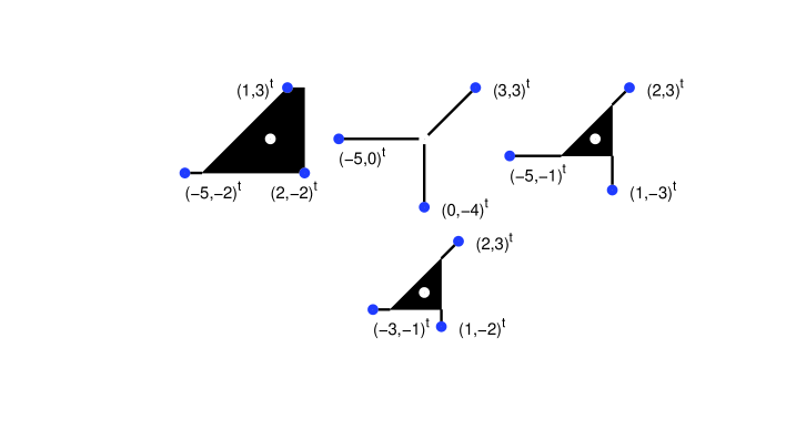
Figure 1: Top: $\{x_{3}=0\}\cap\operatorname{span}A$ (left), $\{x_{3}=0\}\cap\operatorname{span}P(-p,0)$ (center) and $\{x_{3}=0\}\cap\operatorname{span}B$ (right), for $p=(4,3,5)$. Bottom: $\{x_{3}=0\}\cap\operatorname{span}C$, with $C=AB=BA$. In each case, the zero vector is marked in white and generators are represented in blue. The matrices $A,B$ and $C$ are perturbations of $P(-p,0)$.

5 Geometry

Let $A,B\in M_{n}^{nor}$ be real. Here we study the role played by the geometry of the complexes $\operatorname{span}A$ and $\operatorname{span}B$ in order to have $AB=BA$. To do so, we bear in mind how the maps $f_{A}$ and $f_{B}$ act, where $f_{A}:\overline{\mathbb{R}}^{n}\rightarrow\overline{\mathbb{R}}^{n}$ transforms a column vector $X$ into the product $AX$. For $n=3$, $f_{A}$ is described in detail in see [28]; see also [31].

Before, we have met two instances where the geometry explains why $AB=BA$. Namely, in remarks after propositions 7 and 8. In the first (resp. second) case we have $AB=BA=A$ (resp. $AB=BA=B$) because $\operatorname{span}B$ is much larger (resp. smaller) than $\operatorname{span}A$.

More generally, we explore the relationship among the sets $\operatorname{span}A$, $\operatorname{span}B$, $\operatorname{span}(AB)$ and $\operatorname{span}(BA)$ when commutativity is present or absent. In general, we have $\operatorname{span}(AB)\subseteq\operatorname{span}A$ and $\operatorname{span}(BA)\subseteq\operatorname{span}B$. In particular, if $AB=BA$ then $\operatorname{span}(AB)\subseteq\operatorname{span}A\cap\operatorname{span}B$.

Proposition 24.

Let $A,B\in M_{n}^{nor}$. If $A\leq B=B^{2}$ and $A$ is real, then $A\in\Omega^{B}(B)$ and $\operatorname{span}A\supseteq\operatorname{span}B$.

Proof.

By normality, we have $I\leq A\leq B\leq 0$ and left or right tropical multiplication by any matrix is monotonic. Therefore, $B\leq AB\leq B^{2}=B$ and $B\leq BA\leq B^{2}=B$, whence $AB=BA=B$ and $A\in\Omega^{B}(B)$. Moreover, whatever the matrices $A$ and $B$ may be, we have $\operatorname{span}A\supseteq\operatorname{span}(AB)$ and, in our case, $\operatorname{span}(AB)=\operatorname{span}B$. ∎

The hypothesis $B=B^{2}$ cannot be removed in the previous proposition, as the following example shows.

Example 25.

Consider

$$A=\left[\begin{array}[]{rrr}0&-1&-3\\ 0&0&-4\\ 0&0&0\\ \end{array}\right]\leq B=\left[\begin{array}[]{rrr}0&-1&-2\\ 0&0&-4\\ 0&0&0\\ \end{array}\right],$$

then

$$AB=\left[\begin{array}[]{rrr}0&-1&-2\\ 0&0&-2\\ 0&0&0\\ \end{array}\right]\neq BA=\left[\begin{array}[]{rrr}0&-1&-2\\ 0&0&-3\\ 0&0&0\\ \end{array}\right],$$

and $\operatorname{span}A\not\supseteq\operatorname{span}B$; see figure 2.

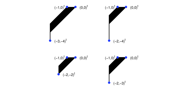
Figure 2: Top: $\{x_{3}=0\}\cap\operatorname{span}A$ (left), $\{x_{3}=0\}\cap\operatorname{span}B$ (right). Bottom: $\{x_{3}=0\}\cap\operatorname{span}(AB)$ (left), $\{x_{3}=0\}\cap\operatorname{span}(BA)$ (right). In this case, $\operatorname{span}A\cap\operatorname{span}B=\operatorname{span}(AB)$. Generators are represented in blue.

Below we explore the properties of the matrices $\underline{A},A$ and $\overline{A}$ and of the corresponding polyhedral complexes.

Example 11.

(Continued) By proposition 17, we have

$$\underline{B}=\left[\begin{array}[]{rrr}0&-3&-3\\ -5&0&-6\\ -5&-2&0\end{array}\right]\leq B=\left[\begin{array}[]{rrr}0&-3&-1\\ -4&0&-6\\ -5&0&0\end{array}\right]\leq\overline{B}=\left[\begin{array}[]{rrr}0&-1&-1\\ -4&0&-5\\ -4&0&0\end{array}\right]$$

and we can easily check, in this case, that

$$\operatorname{span}\underline{B}\supseteq\operatorname{span}B\supseteq\operatorname{span}\overline{B}.$$

See figure 3, where we are using the matrices

$$\underline{B}_{0}=\left[\begin{array}[]{rrr}5&-1&-3\\ 0&2&-6\\ 0&0&0\end{array}\right],B_{0}=\left[\begin{array}[]{rrr}5&-3&-1\\ 1&0&-6\\ 0&0&0\end{array}\right],\overline{B}_{0}=\left[\begin{array}[]{rrr}4&-1&-1\\ 0&0&-5\\ 0&0&0\end{array}\right],$$

as defined in p. 4. Notice that $\{x_{3}=0\}\cap\operatorname{span}B$ is the union of one closed 2–dimensional cell (called soma) and three closed 1–dimensional cells (called antennas); see [28] for the definition of soma, antennas and co–antennas (with a slightly different notation and language). In figure 3, bottom, we can see $\{x_{3}=0\}\cap\operatorname{span}B$ together with its co–antennas.

In this example,

$$\overline{B}=B^{*}$$

and the matrix $\underline{B}$ is idempotent. Therefore, the sets $\operatorname{span}\underline{B}$ and $\operatorname{span}\overline{B}$ are classically convex, and so are the sections $\{x_{3}=0\}\cap\operatorname{span}\underline{B}$ and $\{x_{3}=0\}\cap\operatorname{span}\overline{B}$.

Consider $\mathcal{H}$, the classical convex hull of $\{x_{3}=0\}\cap\operatorname{span}B$: its the vertices are $(5,0)^{t},(5,1)^{t},(-2,1)^{t},(-3,0)^{t},(-3,-6)^{t}$ and $(-1,-6)^{t}$, going counterclockwise. Notice that $\{x_{3}=0\}\cap\operatorname{span}\underline{B}$ is strictly larger than $\mathcal{H}$. Actually, $\{x_{3}=0\}\cap\operatorname{span}\underline{B}$ is the convex hull of the union of $\{x_{3}=0\}\cap\operatorname{span}B$ and the co–antennas of it. On the other hand, $\{x_{3}=0\}\cap\operatorname{span}\overline{B}$ is the soma of $\{x_{3}=0\}\cap\operatorname{span}B$, i.e., it is the maximal convex set contained there.∎

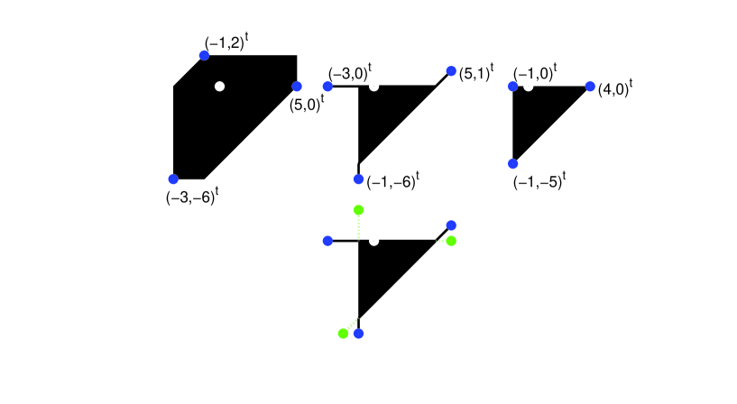
Figure 3: Top: $\{x_{3}=0\}\cap\operatorname{span}\underline{B}$ (left), $\{x_{3}=0\}\cap\operatorname{span}B$ (center) and $\{x_{3}=0\}\cap\operatorname{span}\overline{B}$ (right), for $B$ in (21). In each case, the zero vector is marked in white, and generators (i.e., columns of the corresponding matrix $\underline{B}_{0}$, $B_{0}$ and $\overline{B}_{0}$) are represented in blue. The hyperplane section $\{x_{3}=0\}\cap\operatorname{span}B$ has three antennas. Bottom: $\{x_{3}=0\}\cap\operatorname{span}B$ is represented together with its co–antennas, which appear dotted in green. The convex hull of the bottom figure is the top left one.

We wonder whether the statements in the former example are true for any real $B\in M_{n}^{nor}$. This is an open QUESTION.

References

[1]
[1] M. Akian, R. Bapat and S. Gaubert, Max–plus algebra, chapter 25 in Handbook of linear algebra, L. Hobgen (ed.) Chapman and Hall, 2007.
[2] F.L. Baccelli, G. Cohen, G.J. Olsder and J.P. Quadrat, Syncronization and linearity, John Wiley; Chichester; New York, 1992.
[3] E. Brugallé, Un peu de géométrie tropicale, Quadrature, 74, (2009), 10–22.
[4] E. Brugallé, Some aspects of tropical geometry, Newsletter of the European Mathematical Society, 83, (2012), 23–28.
[5] P. Butkovič, Max–algebra: the linear algebra of combinatorics?, Linear Algebra Appl. 367, (2003), 313–335.
[6] P. Butkovič, Simple image set of linear mappings, Discrete Appl. Math. 105, (2000), 73–86.
[7] P. Butkovič, Max–plus linear systems: theory and algorithms, 2010, Springer.
[8] R. Cuninghame–Green, Minimax algebra, LNEMS, 166, Springer, 1970.
[9] R.A. Cuninghame–Green, Minimax algebra and applications, in Adv. Imag. Electr. Phys., 90, P. Hawkes, (ed.), Academic Press, 1–121, 1995.
[10] M. Develin, B. Sturmfels,
Tropical convexity, Doc. Math.9, (2004) 1–27; Erratum in Doc. Math. 9 (electronic),
(2004) 205–206.
[11] A. Gathmann, Tropical algebraic
geometry, Jahresbericht der DMV, 108, n.1,
(2006), 3–32.
[12] I. Itenberg, E. Brugallé, B. Tessier, Géométrie tropicale, Editions de l’École Polythecnique, 2008.
[13] I. Itenberg, G. Mikhalkin and E. Shustin, Tropical algebraic geometry,
Birkhäuser, 2007.
[14] M. Johnson and M. Kambites, Idempotent tropical matrices and finite metric spaces, to appear in Adv. Geom.; arXiv: 1203.2480, 2012.
[15] Z. Izhakian, M. Johnson and M. Kambites, Pure dimension and projectivity of tropical politopes, arXiv: 1106.4525, 2012.
[16] Z. Izhakian, M. Johnson and M. Kambites, Tropical matrix groups, arXiv: 1203.2449, 2012.
[17] A. Jiménez and M.J. de la Puente, Characterizing the convexity of the –dimensional tropical simplex and the six maximal convex classes in , arXiv: 1205.4162, 2012.
[18] M. Joswig and K. Kulas, Tropical and ordinary convexity combined, Adv. Geom. 10, (2010)
333-352.
[19] M. Joswig, B. Sturmfels and J. Yu, Affine buildings and tropical convexity, Albanian J. Math. 1, n.4, (2007) 187–211.
[20] R. Katz, H. Schneider and S. Sergeev, On commuting matrices in max algebra and in classical nonegative algebra, Linear Algebra Appl. 436, (2012), 276–292.
[21] H.W. Kuhn, The Hungarian method for the assignment problem, Naval Res. Logist. 2, (1955), 83–97.
[22] T. Lam and A. Postnikov,
Alcoved polytopes I, Discrete Comput. Geom., 38 n.3, (2007) 453-478.
[23] T. Lam and A. Postnikov,
Alcoved polytopes II, arXiv:1202.4015v1 (2012).
[25] G. Mikhalkin, What is a tropical curve?, Notices AMS, April 2007, 511–513.
[26] C.H. Papadimitriou and K. Steiglitz, Combinatorial optimization: algorithms and complexity, Prentice Hall, 1982 and corrected unabrideged republication by Dover, 1998.
[27] V.V. Prasolov, Problems and theorems in linear algebra, AMS, 1994.
[28] M. J. de la Puente, Tropical linear maps on the plane,
Linear Algebra Appl. 435, n.7, (2011) 1681–1710.
[29] M. J. de la Puente, On tropical Kleene star matrices and alcoved polytopes, Kybernetika, 49, n.6, (2013) 897–910.
[30] J. Richter–Gebert, B. Sturmfels, T.
Theobald, First steps in tropical geometry, in
[24], 289–317.
[31] F. Rincón,
Local tropical linear spaces, Discrete Comput. Geom. 50, (2013), 700–713.
[32] S. Sergeev, Max–plus definite matrix closures and their eigenspaces, Linear
Algebra Appl. 421, (2007) 182–201.
[33] S. Sergeev, H. Scheneider and P. Butkovič, On visualization, subeigenvectors and Kleene stars in max algebra, Linear Algebra Appl. 431, 2395–2406, (2009).
[34] D. Speyer, B. Sturmfels, Tropical mathematics,
Math. Mag. 82, n.3, (2009) 163–173.
[35] E. Wagneur, Moduloïds and
pseudomodules. Dimension theory, Discr. Math. 98
(1991) 57–73.
[36] A. Werner and J. Yu, Symmetric alcoved polytopes, arXiv: 1201.4378v1 (2012).
[37] M. Yoeli, A note on a generalization of boolean matrix theory, Amer. Math. Monthly 68, n.6,
(1961) 552–557.
[38] K. Zimmermann, Extremální algebra, Výzkumná publikace ekonomicko–matematické laboratoře při ekonomickém ústavé ČSAV, 46, Prague, 1976, in Czech.